Current address : ]Research Unit Lasers and Spectroscopies (UR-LLS), naXys & NISM, University of Namur, Rue de Bruxelles 61, B-5000 Namur, Belgium

Relativistic Quantum Field Theory Approach to Wavepacket Tunneling: Lack of Superluminal Transmission

M. Alkhateeb Laboratoire de Physique Théorique et Modélisation, CNRS Unité 8089, CY Cergy Paris Université, 95302 Cergy-Pontoise cedex, France [    X. Gutierrez de la Cal Departmento de Química-Física, Universidad del País Vasco, UPV/EHU, 48940 Leioa, Spain EHU Quantum Center, Universidad del País Vasco, UPV/EHU, 48940 Leioa, Spain    M. Pons EHU Quantum Center, Universidad del País Vasco, UPV/EHU, 48940 Leioa, Spain Departamento de Física Aplicada, Universidad del País Vasco, UPV/EHU, 48013 Bilbao, Spain    D. Sokolovski Departmento de Química-Física, Universidad del País Vasco, UPV/EHU, 48940 Leioa, Spain EHU Quantum Center, Universidad del País Vasco, UPV/EHU, 48940 Leioa, Spain IKERBASQUE, Basque Foundation for Science, E-48011 Bilbao, Spain    A. Matzkin Laboratoire de Physique Théorique et Modélisation, CNRS Unité 8089, CY Cergy Paris Université, 95302 Cergy-Pontoise cedex, France
Abstract

We investigate relativistic wavepacket dynamics for an electron tunneling through a potential barrier employing space-time resolved solutions to relativistic quantum field theory (QFT) equations. We prove by linking the QFT property of micro-causality to the wavepacket behavior that the tunneling dynamics is fully causal, precluding instantaneous or superluminal effects that have recently been reported in the literature. We illustrate these results by performing numerical computations for an electron tunneling through a potential barrier for standard tunneling as well for Klein tunneling. In all cases (Klein tunneling  or regular tunneling across a standard or a supercritical potential) the transmitted wavepacket remains in the causal envelope of the propagator, even when its average position lies ahead of the average position of the corresponding freely propagated wavepacket.

Tunneling is one of the most intriguing quantum phenomena. Although tunneling underlies many important processes in about every area concerned by quantum physics (see e.g. [1, 2, 3, 4, 5, 6, 7] for recent observations), its precise mechanism has remained controversial [8, 9]. Despite experimental data coming from different areas, from strong field tunneling ionization [10, 11, 12, 2, 5] to cold atoms [3] neutron optics [13] or condensed matter [14], there seems to be no solution in view [15] to the tunneling time problem (the time spent by a particle inside the barrier), or equivalently the arrival time (whether a particle that tunnels through a barrier arrives earlier than a freely propagating particle). Indeed, due to the ambiguity of measuring time in quantum mechanics – there is no time operator in the standard formalism – any observed tunneling time will depend on the model employed to extract the time interval from the observed data.

In particular, experiments involving electron photo-ionization have reported results interpreted to indicate instantaneous tunneling times [10, 11, 2, 5]. Such interpretations rely on models that intrinsically involve disputed approximations [16], generally employing a non-relativistic and often semiclassical framework. Perhaps somewhat more surprisingly, several works based on a first-quantized relativistic framework [17, 18, 19, 20, 21, 22, 23, 24, 25] have concluded on the possibility of superluminal arrival times for electrons. Such superluminal transmissions could potentially bring serious issues with causality, even though it is sometimes asserted that these effects do not seem to lead to signaling [24]. Other investigations carried out within first quantized relativistic quantum mechanics have on the contrary not noted any superluminal effects at the level of the wavefunction [26, 27, 28].

In this work, we investigate the tunneling dynamics in a second quantized framework. More specifically, we will employ a computational relativistic quantum field theory (QFT) approach in order to follow the space-time resolved dynamics of an electron tunneling through an electrostatic potential barrier represented by a background field. The electron is modeled as a wave-packet initially defined on a compact support launched towards a potential barrier. We will prove that micro-causality of the fermionic quantum field implies that the electron wavepacket density evolves causally, thereby ensuring the absence of any superluminal effects such as instantaneous tunneling times. The present method allows us to treat on the same footing different types of tunneling effects: the familiar one characterized by exponentially decaying waves inside the barrier, as well as Klein tunneling (with undamped oscillating waves in the barrier) for supercritical barriers (that is barriers with a potential above the pair-production threshold).

Our approach is based on a computational QFT framework [29], recently extended to treat particle scattering across a finite barrier [30] (see also [32, 31] for related recent work). Since we are interested in studying possibly superluminal phenomena, it makes sense [33] to take initially ($t=0$) a wavepacket defined over a compact support. As is well-known [34, 35], a relativistic quantum state defined on a compact spatial support must contain both positive and negative energy components, so that the initial state in Fock space is defined by

$$\|\chi\rrangle=\int dp\big{(}g_{+}(p)b_{p}^{\dagger}+g_{-}(p)d_{p}^{\dagger}\big{)}\|0\rrangle.$$ (1)

Here $b_{p}^{\dagger}(t)$ and $d_{p}^{\dagger}(t)$ are the creation operators for a particle and antiparticle of momentum $p$, and $b_{p}(t)$ (resp. $d_{p}(t))$ are the corresponding annihilation operators; $\|0\rrangle$ defines the vacuum state, i.e. $b_{p}\|0\rrangle=d_{p}\|0\rrangle=0$, and $g_{\pm}(p)$ are the expansion coefficients in momentum space. Since we are dealing with a Dirac field the creation and annihilation operators anti-commute, $[b_{p},b_{k}^{\dagger}]_{+}=[d_{p},d_{k}^{\dagger}]_{+}=\delta(p-k)$.

The particle density at any given time is given by the expectation value

$$\rho(t,x)=\llangle\chi\|\hat{\rho}(t,x)\|\chi\rrangle$$ (2)

where the density operator $\hat{\rho}(t,x)$ is defined by

$$\hat{\rho}(t,x)=\hat{\Phi}^{\dagger}(t,x)\hat{\Phi}(t,x).$$ (3)

$\hat{\Phi}(t,x)$ is the field operator suited to obtain the evolved compact support Fock space state $\hat{\Phi}(t,x)=\int dpb_{p}(t)v_{p}(x)+\int dpd_{p}(t)w_{p}(x).$ $v_{p}(x)$ and $w_{p}(x)$ are resp. the positive and negative energy spinor eigenfunctions of the field-free Dirac Hamiltonian [see Eq. (A-3) of Appdx A]. The free Dirac Hamiltonian $H_{0}=-i\hbar c\alpha_{x}\partial_{x}+\beta mc^{2}$ has the corresponding eigenvalues $\pm\left|E_{p}\right|=\pm\sqrt{p^{2}c^{2}+m^{2}c^{4}}$ ($\alpha$ and $\beta$ are the usual Dirac matrices 111In one spatial dimension, we can neglect spin-flip and replace $\alpha_{x}$ and $\beta$ by the Pauli matrices $\sigma_{1}$ and $\sigma_{3}$ respectively., $m$ the electron mass and $c$ the light velocity). The equal-time anti-commutators obey

$$[\hat{\Phi}^{\dagger}(t,x^{\prime}),\hat{\Phi}(t,x)]_{+}=\delta(x^{\prime}-x)$$ (4)

just like the familiar field operators of the free Dirac field [36] (see Appendix A for the proof of Eq. (4) and the relation to the familiar QFT case). The time-dependent creation and annihilation operators are obtained as prescribed by our computational QFT method through [29]

$\displaystyle b_{p}(t)$ $\displaystyle=\int dk\left(U_{v_{p}v_{k}}(t)b_{k}(0)+U_{v_{p}w_{k}}(t)d_{k}^{\dagger}(0)\right)$ (5)
$\displaystyle d_{p}^{\dagger}(t)$ $\displaystyle=\int dk\left(U_{w_{p}v_{k}}(t)b_{k}(0)+U_{w_{p}w_{k}}(t)d_{k}^{\dagger}(0)\right).$ (6)

$U$ is the unitary evolution operator of the full Hamiltonian $H=H_{0}+V(x).$ The barrier potential $V(x)$ is treated as background external field [37]. We will work for convenience with a rectangular-like model potential $V(x)=\frac{V_{0}}{2}\left[\tanh(\left(x+L/2\right)/\epsilon)-\tanh(\left(x-L/2\right)/\epsilon)\right]$ where $L$ is the barrier width and $\epsilon$ a smoothness parameter. The unitary evolution operator elements, $U_{v_{k}w_{p}}(t)\equiv\left\langle v_{k}\right|\exp\left(-iHt/\hbar\right)\left|w_{p}\right\rangle$ are computed numerically on a discretized space-time grid using a split operator [38] method (the evolution operator is split into a kinetic part propagated in momentum space and a potential-dependent part solved in position space).

Refer to caption
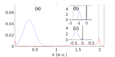
Figure 1: (a) The density of the transmitted wavepacket is shown (dotted blue) as it is exiting the barrier ($t=1.5\times 10^{-2}$ a.u.) for a comparatively low potential ($V_{0}=0.5mc^{2}$) giving rise to standard tunneling, with a negligible pair creation rate (the electron density created by the potential is shown in red). The inset displays snapshots of the wavepacket dynamics at (b) $t=0$ and at (c) $t=1.5\times 10^{-2}$ a.u (note the transmitted wavepacket is hardly visible on that scale in (c)). The dotted vertical line in (b) represents the right edge of the support $\mathcal{D}$ over which the initial wavepacket is defined. The same line in (a) and (c) represents the position of the light-cone emanating from this right edge at the time of the plot. The initial wavepacket parameters in atomic units (a.u.) are $x_{0}=-120\lambda$, $p_{0}=100$ a.u. and $\mathcal{D}=70\lambda$ and for the barrier $L=4\lambda$ and $\varepsilon=0.3\lambda$, where $\lambda=\hbar/mc$ is the Compton wavelength of the electron.

An example of such a computation is shown in Fig. 1. An initial wave-packet given by the Dirac spinor $G(x)=\left(\cos^{8}(\frac{x-x_{0}}{D})e^{ip_{0}x},0\right)$ is defined to be non-zero only over the compact support $x\in\mathcal{D}$ where $\mathcal{D}=[x_{0}-D\pi/2,x_{0}+D\pi/2]$ is localized to the left of the barrier, with an initial mean momentum such that the electron wave-packet moves towards the right as time evolves. By projecting this spatial profile over the free Dirac basis $v_{p}(x)$ and $w_{p}(x)$ we obtain the coefficients $g_{\pm}(p)$ of Eq. (1) needed to define the initial second quantized wave-packet222Recall that the first quantized wavepacket is obtained from the Fock space state through $\chi(t,x)=\llangle 0\|\hat{\Phi}(t,x)\|\chi\rrangle$ [39, 40] which is in turn fed in Eq. (2) in order to obtain the space-time resolved density $\rho(t,x)$. $\rho(t,x)$ can be parsed in several ways (see Appendix B). In particular for distances sufficiently far from the barrier, the density represents the sum of the transmitted or reflected electron wavepacket and the electron density due to pair production (which is asymptotically small for barriers of height $V_{0}\ll 2mc^{2}$).

Fig. 1 shows the transmitted wavepacket as well as the electron density due to pair production for a comparatively “low” potential (V0=0.5mc2subscript𝑉00.5𝑚superscript𝑐2V_{0}=0.5mc^{2}). Snapshots of the density evolution are given in the inset; leaving aside pair production, this situation is a QFT account of the familiar tunneling dynamics, where most of the incoming electron amplitude is reflected and only a very small amplitude 
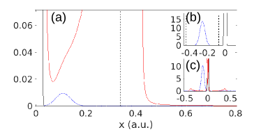
is transmitted. Fig. 2 shows the situation for a higher barrier (V0=1.77mc2subscript𝑉01.77𝑚superscript𝑐2V_{0}=1.77mc^{2}) at tp=3×10³subscript𝑡𝑝3superscript103t_{p}=3\times 10^{-3} a.u.: pair-production is still small (the total number of electrons due to pair production is Nvac(tp)/2=0.31subscript𝑁𝑣𝑎𝑐subscript𝑡𝑝20.31N_{vac}(t_{p})/2=0.31 [see Eq. (A-33) of Appdx B]), but the transmitted wavepacket amplitude is even smaller and overshadowed by the electron density produced by the barrier and appears as a bump in the overall electron density. Note that some of the works [17, 18, 19, 20, 21, 22, 23, 24, 25] investigating relativistic tunneling within the first quantized approximation have computed numerical results for barrier heights in cases in which QFT calculations show that the tiny amplitude of the transmitted wavepacket is completely obscured by the larger (or much larger if supercritical barriers are considered) electron density produced by the barrier.

Refer to caption
Figure 2: Similar to Fig. 1 but for a stronger potential $V_{0}=1.77mc^{2}$. (a) The density of the transmitted wavepacket (dotted blue) is overshadowed by the electron density due to pair creation and appears as a bump in the overall particle density (shown in red). The inset displays snapshots of the wavepacket dynamics at (b) $t=0$ and at (c) $t=3\times 10^{-3}$ (the time of the plot (a)). The initial wavepacket parameters are (in a.u.) $x_{0}=-35\lambda$, $p_{0}=200$ and $\mathcal{D}=16\lambda$ and for the barrier $L=4\lambda$ and $\varepsilon=0.3\lambda$, where $\lambda=\hbar/mc$.

Fig. 2 also shows the light cone, emanating from the right edge ($x=x_{0}+D\pi/2$) of the initial wavepacket density distribution; it can be seen that although  the electron is in the relativistic regime (the mean velocity of the initial distribution is $0.83c$), the transmitted wavepacket remains well inside the light cone. This is an illustration of a very general result hinging on micro-causality of relativistic quantum fields: observables that are space-like separated commute. If $O(t,x)$ and $O^{\prime}(t^{\prime},x^{\prime})$ are two obervables, $[\hat{O}^{\prime},\hat{O}]=0\;\;$for$\;\;c^{2}\left(t^{\prime}-t\right)^{2}-\left(x^{\prime}-x\right)^{2}<0$, thereby implying that observations made at space-like separated points are independent. It is straightforward to verify that micro-causality holds here: by recalling that a general observable is built from a bilinear form of field operators [36, 41], the commutator $[\hat{O}^{\prime},\hat{O}]$ for arbitrary observables can be seen to be proportional to the field anti-commutator $[\hat{\Phi}^{\dagger}(t^{\prime},x^{\prime}),\hat{\Phi}(t,x)]_{+}$ (a particular instance is given in Eq. (A-13) of Appdx A for the important case of density observables). These field anti-commutators vanish for space-like separated points: this can be seen by Lorentz-boosting (to another reference frame for which $t^{\prime}\neq t$) the equal-time anti-commutator of Eq. (4). As proved in Appendix A, this anti-commutator vanishes for space-like separated events for the free case and also in the presence of background fields.

Refer to caption
Figure 3: Similar to Figs. 1 and 2 but for a potential $V_{0}=9mc^{2}$ above the supercritical limit, giving rise to Klein tunneling. (a) The electron wavepacket density is shown (dotted blue) at $t=4.5\times 10^{-3}$ a.u. well after the transmitted wavepacket (centered at $x\approx 0.3$ a.u.) has exited the barrier (solid vertical lines). Note that the transmitted wavepacket density is significantly larger than the one of the reflected wavepacket (centered at $x=-0.19$ a.u. and moving toward the left). (b) The initial wavepacket (light blue) is shown along with the support $\mathcal{D}$ (dashed lines) and the barrier. (c) The plot (a) is zoomed out in order to visualize the electron density due to pair production (red line). The wavepacket is not visible at this scale. The initial wavepacket parameters in a.u. are $x_{0}=-40\lambda$,$p_{0}=450$ a.u. and $\mathcal{D}=16\lambda$ and for the barrier $L=16\lambda$ and $\varepsilon=0.3\lambda$ with $\lambda=\hbar/mc$.

We can now show that micro-causality imposes the causality of the tunneling dynamics in the following way. Let us choose $\hat{O}$ as an intervention on the wavepacket density at $t=0,$ $\hat{O(0,\mathcal{D})}=\int_{\mathcal{D}}dx\hat{\Phi}^{\dagger}(0,x)f(x)\hat{\Phi}(0,x)$ where $f(x)$ is an arbitrary positive-definite real function that modifies the profile of the initial wavepacket. $O$ is now defined over the domain $\mathcal{D}$ rather than at a single point $x$. Note that $f(x)$ must be chosen such that $\llangle\chi\|\hat{O}\|\chi\rrangle=\int_{\mathcal{D}}dxf(x)\chi^{\dagger}(x)\chi(x)$ remains normalized. We will set $\hat{O}^{\prime}=\hat{\rho}(t^{\prime},x^{\prime})$ to be the density [Eq. (3)] at a space-like separated point $(x^{\prime}>c\left(t^{\prime}-t\right)+x_{0}+D\pi/2$) to the right of the barrier and sufficiently far from it $\left(x^{\prime}\gg L/2\right)$. Note that $x_{0}+D\pi/2$ being the right edge of $\mathcal{D}$, any point of the initial wavepacket density is space-like separated form $(t^{\prime},x^{\prime})$. By relying on micro-causality, it can be established that

$$\llangle\chi\|\hat{O}^{\prime}(t^{\prime},x^{\prime})\hat{O}(0,\mathcal{D})\|\chi\rrangle=\llangle 0\|\hat{O}^{\prime}(t^{\prime},x^{\prime})\|0\rrangle.$$ (7)

This means that the electron density at $(t^{\prime},x^{\prime})$ is given by a vacuum expectation value and does not depend in any way on the initial wavepacket density or any operation one would perform on the wavepacket at $t=0$ (the vacuum density is non-vanishing due to the electrons produced by the barrier). These results are proved in Appendix C.

Eq. (7) linking the causal behavior of the tunneled wavepacket to micro-causality is our main theoretical result and implies that tunneling cannot be superluminal nor instantaneous once relativistic QFT constraints are taken into account. It is noteworthy that this result does not depend on the shape, width or height of the background potential (see Appendix C) – it also holds in particular for more complicated potentials than the smooth rectangular barrier we have employed here. This result holds of course for all types of tunneling – for regular tunneling, as in Figs. 1 or 2, or for Klein tunneling.

Klein tunneling takes place for supercritical potentials ($V_{0}>2mc^{2}$) and wavepacket energies for which $\left(E-V_{0}\right)^{2}>m^{2}c^{4}$; in this case the transmission of the electron wavepacket is mediated by pair production [42, 30] giving rise to an oscillating density inside the barrier. These modulations in pair-production give rise to a transmitted wavepacket with an undamped amplitude (as opposed to an exponentially decreasing tranmission in the case of regular tunneling). Relative to the freely propagated wavepacket, the transmitted Klein tunneled one can be accelerated by the barrier (since the negative energy wavepacket components see a potential well [43]) but never faster than light, since our result Eq. (7) holds for any type of potential barrier. A computation illustrating Klein tunneling is given in Fig. 3, for $V_{0}=9mc^{2}$.

Refer to caption
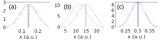
Figure 4: (a), (b) and (c) display for each case considered respectively in Figs. 1, 2 and 3, the position of the transmitted peak along with the position of the same initial wavepacket that would have evolved freely. The vertical dotted lines indicate the averages $\left\langle X_{\mathrm{tr}}(t)\right\rangle$ and $\left\langle X_{\mathrm{free}}(t)\right\rangle$ (see text for details).

Finally, since it is often stated that tunneling can be superluminal and we have shown here that this is contrary to the predictions obtained from a space-time resolved relativistic QFT approach to spin-1/2 fermions, it is worthwhile briefly recalling on which gounds such assertions have been made. We must first discard models based on non-relativistic frameworks, like the Schrödinger equation, for which propagation is indeed instantaneous [44], or semi-classical approximations to it. Experimental results, in particular those involving the attoclock technique in strong field ionization (see e.g. [10, 11, 2, 5]), have usually relied on such models when estimating tunneling times. Second, there is no unambiguous manner to define a tunneling time [15] and the various quantities that have been proposed (phase delays, dwell times, Larmor times, time operators) lead to conflicting results and may by construction yield superluminal values, including when they are employed with relativistic wave equations [17, 19, 20, 21, 23, 25].

Third, some first quantized works based on relativistic wave equations have suggested [18, 24] superluminal transmission based on the fact that the transmitted wavepacket arrives on average earlier than the freely propagating one, i.e. $\left\langle X_{\mathrm{tr}}(t)\right\rangle>\left\langle X_{\mathrm{free}}(t)\right\rangle$ where in $\left\langle X_{\mathrm{tr}}(t)\right\rangle$ the average is taken over the transmitted peak only (it is a conditional expectation value). Asserting that the transmitted wavepacket travels faster on this basis is only possible if one associates a conditional wavepacket (the transmitted one) with a single particle. While reasoning in this manner might be disputed even from within a standard quantum mechanics perspective (it is far from obvious that a fraction of a wavefunction can be associated with a single particle), it is clearly not compatible with a QFT based framework. According to QFT, a particle at each space-time point of a wavepacket is seen as a field excitation at that particular point, and the field excitation at that point is causally related to the field excitation at some other space-time point, in particular to the field excitation at a different position in a given reference frame. In the three numerical examples given here we also have $\left\langle X_{\mathrm{tr}}(t)\right\rangle>\left\langle X_{\mathrm{free}}(t)\right\rangle$ (see Fig. 4) while still being constrained by Eq. (7).

To sum up, we have investigated the tunneling wavepacket dynamics for an electron within a relativistic QFT framework in which the barrier is modeled as a background field. We have shown that if the electron wavepacket is initially ($t=0$) localized to the left of the barrier, the electron density at a space-like separated point to the right of the barrier does not depend on the presence or absence of the wavepacket at $t=0,$ thereby precluding any superluminal effects related to tunneling. We have numerically computed the space-time resolved electron density in typical cases of tunneling with potentials below, close to or above the supercritical value. We hope our results will contribute in clarifying the models and approximations employed when accounting for results involving traversal or detection times in tunneling related effects.


Acknowledgments. We are grateful for grant PID2021-126273NB-I00, funded by MCIN/AEI/10.13039/ 501100011033 and “ERDF A way of making Europe”. We acknowledge financial support from the Basque Government, grant No. IT1470-22. MP acknowledges support from the Spanish Agencia Estatal de Investigacion, grant No. PID2022-141283NB-100.


References

  • [1] M. Garg and K. Kern, Attosecond coherent manipulation of electrons in tunneling microscopy, Science 367, 411 (2019).
  • [2] Sainadh, U.S., Xu, H., Wang, X. et al. Attosecond angular streaking and tunnelling time in atomic hydrogen. Nature 568, 75 (2019).
  • [3] David C. Spierings and Aephraim M. Steinberg, Observation of the Decrease of Larmor Tunneling Times with Lower Incident Energy, Phys. Rev. Lett. 127, 133001 (2021).
  • [4] Zhenning Guo, Yiqi Fang, Peipei Ge, Xiaoyang Yu, Jiguo Wang, Meng Han, Qihuang Gong, and Yunquan Liu, Probing tunneling dynamics of dissociative H2 molecules using two-color bicircularly polarized fields, Phys. Rev. A 104, L051101 (2021).
  • [5] Yu, M., Liu, K., Li, M. et al., Full experimental determination of tunneling time with attosecond-scale streaking method, Light Sci Appl 11, 215 (2022).
  • [6] Yoo Kyung Lee, Hanzhen Lin, and Wolfgang Ketterle, Spin Dynamics Dominated by Resonant Tunneling into Molecular States, Phys. Rev. Lett. 131, 213001 (2023).
  • [7] Mirza M. Elahi, Hamed Vakili, Yihang Zeng, Cory R. Dean, and Avik W. Ghosh, Direct Evidence of Klein and Anti-Klein Tunneling of Graphitic Electrons in a Corbino Geometry, Phys. Rev. Lett. 132, 146302 (2024).
  • [8] J. G. Muga and C. R. Leavens, Arrival time in quantum mechanics, Phys. Rep. 338, 353 (2000).
  • [9] U Satya Sainadh, R T Sang and I V Litvinyuk, Attoclock and the quest for tunnelling time in strong-field physics, J. Phys. Photonics 2 042002 (2020).
  • [10] P. Eckle, A. N. Pfeiffer, C. Cirelli, A. Staudte, R. Dᅵrner, H. G. Muller, M. Bᅵttiker, and U. Keller, Science 322, 1525 (2008).
  • [11] Pfeiffer, A., Cirelli, C., Smolarski, M. et al. Attoclock reveals natural coordinates of the laser-induced tunnelling current flow in atoms. Nature Phys 8, 76–80 (2012).
  • [12] Tomᅵᅵ Zimmermann, Siddhartha Mishra, Brent R. Doran, Daniel F. Gordon, and Alexandra S. Landsman, Tunneling Time and Weak Measurement in Strong Field Ionization, Phys. Rev. Lett. 116, 233603 (2016).
  • [13] Masahiro Hino, Norio Achiwa, Seiji Tasaki, Toru Ebisawa, Takeshi Kawai, Tsunekazu Akiyoshi, and Dai Yamazaki, Phys. Rev. A 59, 2261 (1999).
  • [14] P. Fevrier and J. Gabelli, Tunneling time probed by quantum shot noise, Nat Commun 9, 4940 (2018).
  • [15] D. Sokolovski and E. Akhmatskaya, No time at the end of the tunnel. Commun Phys 1, 47 (2018).
  • [16] M. Klaiber, Q. Z. Lv, S. Sukiasyan, D. Bakucz Canario, K. Z. Hatsagortsyan, and C. H. Keitel, Reconciling Conflicting Approaches for the Tunneling Time Delay in Strong Field Ionization, Phys. Rev. Lett. 129, 203201 (2022).
  • [17] P. Krekora, Q. Su, and R. Grobe, Effects of relativity on the time-resolved tunneling of electron wave packets, Phys. Rev. A 63, 032107 (2001).
  • [18] V. Petrillo and D. Janner, Relativistic analysis of a wave packet interacting with a quantum-mechanical barrier, Phys. Rev. A 67, 012110 (2003).
  • [19] Herbert G. Winful, Moussa Ngom, and Natalia M. Litchinitser, Relation between quantum tunneling times for relativistic particles, Phys. Rev. A 70, 052112 (2004); Erratum Phys. Rev. A 108, 019902 (2023).
  • [20] S. De Leo and P.P. Rotelli, Dirac equation studies in the tunneling energy zone, Eur. Phys. J. C 51, 241 (2007).
  • [21] A. E. Bernardini, Delay time computation for relativistic tunneling particles, Eur. Phys. J. C 55, 125 (2008).
  • [22] O. del Barco and V Gasparian, Relativistic tunnelling time for electronic wave packets, J. Phys. A: Math. Theor. 44 015303 (2011).
  • [23] S. De Leo, A study of transit times in Dirac tunneling, J. Phys. A: Math. Theor. 46 15530 (2013).
  • [24] R. S. Dumont, T. Rivlin, and E. Pollak, The relativistic tunneling flight time may be superluminal, but it does not imply superluminal signaling, New J. Phys. 22, 093060 (2020).
  • [25] P. C. Flores and E. A. Galapon, Instantaneous tunneling of relativistic massive spin-0 particles, EPL 141 10001 (2023).
  • [26] J. C. Park and Y. J. Lee, Superluminality and Causality in the Relativistic Barrier Problem, J. Korean Phys. Soc. 43, 4 (2003).
  • [27] M. Alkhateeb, X. Gutierrez de la Cal, M. Pons, D. Sokolovski and A. Matzkin, Relativistic time-dependent quantum dynamics across supercritical barriers for Klein-Gordon and Dirac particles, Phys. Rev. A 103, 042203 (2021).
  • [28] L. Gavassino and M. M. Disconzi, Subluminality of relativistic quantum tunneling, Phys. Rev. A 107, 032209 (2023).
  • [29] T. Cheng, Q. Su, and R. Grobe, Introductory review on quantum field theory with space–time resolution, Contemp. Phys. 51, 315 (2010).
  • [30] M. Alkhateeb and A. Matzkin, Space-time-resolved quantum field approach to Klein-tunneling dynamics across a finite barrier, Phys. Rev. A 106, L060202 (2022).
  • [31] D. D. Su, Y. T. Li, Q. Z. Lv, and J. Zhang, Enhancement of pair creation due to locality in bound-continuum interactions, Phys. Rev. D 101, 054501 (2020).
  • [32] J. Unger, S. Dong, Q. Su, and R. Grobe, Optimal supercritical potentials for the electron-positron pair-creation rate, Phys. Rev. A 100, 012518 (2019).
  • [33] M. V. Berry, Causal wave propagation for relativistic massive particles: physical asymptotics in action, Eur. J. Phys. 33 279 (2012).
  • [34] H. Feschbach and F. Villars, Elementary Relativistic Wave Mechanics of Spin 0 and Spin 1/2 Particles, Rev. Mod. Phys. 30, 24 (1958).
  • [35] Stephen A. Fulling, Aspects of Quantum Field Theory in Curved Spacetime (Cambdrige Univ. Press, Cambridge, Great Britain, 1989).
  • [36] W. Greiner, Field Quantization (Springer-Verlag, Berlin, 1996).
  • [37] S. P. Gavrilov and D. M. Gitman, Consistency Restrictions on Maximal Electric-Field Strength in Quantum Field Theory, Phys. Rev. Lett. 101, 130403 (2008).
  • [38] M. Ruf, H. Bauke and C. H. Keitel, J. Comp. Phys. 228 9092 (2009).
  • [39] S. S. Schweber, An Introduction to Relativistic Quantum Field Theory (Dover, New York, 2005).
  • [40] M. Alkhateeb and A. Matzkin, Evolution of strictly localized states in noninteracting quantum field theories with background fields, Phys. Rev. A 109, 062223 (2024).
  • [41] Thanu Padmanabhan, Quantum Field Theory (Springer International Publishing Switzerland, 2016).
  • [42] P. Krekora, Q. Su, and R. Grobe, Klein Paradox in Spatial and Temporal Resolution, Phys. Rev. Lett. 92, 040406 (2004).
  • [43] N. Dombey and A. Calogeracos, Seventy years of the Klein paradox, Phys. Rep. 315, 41 (1999).
  • [44] Gerhard C. Hegerfeldt and Simon N. M. Ruijsenaars, Remarks on causality, localization, and spreading of wave packets, Phys. Rev. D 22, 377 (1980).

Appendix A - Field operators and equal-time anti-commutators

The field operator $\hat{\Phi}(t,x)$ is given in terms of the annihilation operators of particles and antiparticles by:

$$\hat{\Phi}(t,x)=\int dp\left(\hat{b}_{p}(t)v_{p}(x)+\hat{d}_{p}(t)w_{p}(x)\right)$$ (A-1)

and its Hermitian conjugate applied to the dual Fock states is given by:

$$\hat{\Phi}^{\dagger}(t,x)=\int dp\left(\hat{b}_{p}^{\dagger}(t)v_{p}^{\dagger}(x)+\hat{d}_{p}^{\dagger}(t)w_{p}^{\dagger}(x)\right),$$ (A-2)

where $v_{p}(x)$ and $w_{p}(x)$ are the solutions of the free Dirac equation in one spatial dimension given by

$$\begin{split}v_{p}(x)&=\begin{pmatrix}1\\ \frac{cp}{mc^{2}+E_{p}}\end{pmatrix}e^{ipx}\\ w_{p}(x)&=\begin{pmatrix}1\\ \frac{cp}{mc^{2}-E_{p}}\end{pmatrix}e^{-ipx}\end{split}$$ (A-3)

In the field free case, the time evolution of the creation and annihilation operators is trivial ($\hat{b}_{p}(t)=e^{iE_{p}t}\hat{b}_{p}$, $\hat{d}_{p}^{\dagger}(t)=e^{-iE_{p^{\prime}}t}\hat{d}_{p}^{\dagger}$, etc.)  and the equal-time anti-commutator reads

$$\begin{split}&\left[\hat{\Phi}^{\dagger}(x),\hat{\Phi}(y)\right]_{+}=\\ &\left[\int dp\hat{b}_{p}^{\dagger}v_{p}^{\dagger}(x)e^{iE_{p}t}+\int dp\hat{d}_{p}^{\dagger}w_{p}^{\dagger}(x)e^{-iE_{p}t},\int dp^{\prime}\hat{b}_{p^{\prime}}v_{p^{\prime}}(y)e^{-iE_{p^{\prime}}t}+\int dp\hat{d}_{p^{\prime}}w_{p^{\prime}}(y)e^{-iE_{p^{\prime}}t}\right]_{+}\end{split}$$ (A-4)

Using the anti-commutation relations

$$\begin{split}[\hat{b}_{p}^{\dagger},\hat{b}_{p^{\prime}}]_{+}&=[\hat{d}_{p}^{\dagger},\hat{d}_{p^{\prime}}]_{+}=\delta(p-p^{\prime}),\\ [\hat{b}_{p}^{\dagger},\hat{d}_{p^{\prime}}]_{+}&=[\hat{d}_{p}^{\dagger},\hat{b}_{p^{\prime}}]_{+}=\delta(p-p^{\prime}),\end{split}$$ (A-5)

and

$$\begin{split}v_{p}^{\dagger}(x)v_{p}(y)&=e^{ip(y-x)}\\ w_{p}^{\dagger}(x)w_{p}(y)&=e^{-ip(x-y)},\end{split}$$ (A-6)

we obtain

$$\left[\hat{\Phi}^{\dagger}(x),\hat{\Phi}(y)\right]_{+}=\int dp(e^{ip(y-x)}+e^{ip(x-y)})$$ (A-7)

which leads to Eq. (4).

In the presence of a background potential, the equal-time anti-commutation relation

$$\left[\hat{\Phi}^{\dagger}(t,x),\hat{\Phi}(t,y)\right]_{+}=\left[\int dp\left(\hat{b}_{p}^{\dagger}(t)v_{p}^{\dagger}(x)+\hat{d}_{p}^{\dagger}(t)w_{p}(x)^{\dagger}\right),\int dp\left(\hat{b}_{p}(t)v_{p}(x)+\hat{d}_{p}(t)w_{p}(x)\right)\right]_{+}$$ (A-8)

invoves the anti-commutators of the type

$$\begin{split}&[\hat{b}_{p_{1}}^{\dagger}(t),b_{p_{2}}(t)]=\\ &\left[\int dp_{1}^{\prime}\left(U_{v_{p_{1}}w_{p_{1}^{\prime}}}^{\ast}\hat{b}_{p_{1}^{\prime}}^{\dagger}+U_{v_{p_{1}}w_{p_{1}^{\prime}}}^{\ast}\hat{d}_{p_{1}^{\prime}}\right),\int dp_{2}^{\prime}\left(U_{v_{p_{2}}v_{p_{2}^{\prime}}}\hat{b}_{p_{2}^{\prime}}+U_{v_{p_{2}}w_{p_{2}^{\prime}}}\hat{d}_{p_{2}^{\prime}}^{\dagger}\right)\right]_{+}.\end{split}$$ (A-9)

Using Eq. (5), one obtains

$$\begin{split}&\left[\hat{b}_{p_{1}}^{\dagger}(t),b_{p_{2}}(t)\right]_{+}\\ &=\int d_{p_{1}^{\prime}}\left(U_{v_{p_{1}}v_{p_{1}^{\prime}}}^{\ast}U_{v_{p_{2}}v_{p_{1}^{\prime}}}+U_{v_{p_{1}}w_{p_{1}^{\prime}}}^{\ast}U_{v_{p_{2}}w_{p_{1}^{\prime}}}\right)\\ &=\int d_{p_{1}^{\prime}}\left(\langle v_{p_{2}}|\hat{U}|v_{p_{1}^{\prime}}\rangle\langle v_{p_{1}^{\prime}}|\hat{U}^{\dagger}|v_{p_{1}}\rangle+\langle v_{p_{2}}|\hat{U}|w_{p_{1}^{\prime}}\rangle\langle w_{p_{1}^{\prime}}|\hat{U}^{\dagger}|v_{p_{1}}\rangle\right)\\ &=\langle v_{p_{2}}|\hat{U}\hat{U}^{\dagger}|v_{p_{1}}\rangle=\langle v_{p_{2}}|v_{p_{1}}\rangle=\delta(p_{1}-p_{2}),\end{split}$$ (A-10)

where in the last line, we used the completeness relation:

$$\int dp^{\prime}\left(|v_{p^{\prime}}\rangle\langle v_{p^{\prime}}|+|w_{p^{\prime}}\rangle\langle w_{p^{\prime}}|\right)=1$$

and the orthonormality of the solutions of the free Dirac equation. Similarly, we find that

$$\left[\hat{d}_{p_{1}}^{\dagger}(t),d_{p_{2}}(t)\right]_{+}=\delta(p_{1}-p_{2}).$$ (A-11)

Pluging-in these anti-commutators into Eq. (A-8) leads to

$$\left[\hat{\Phi}^{\dagger}(t,x),\hat{\Phi}(t,y)\right]_{+}=\int dp(e^{ip(y-x)}+e^{ip(x-y)})$$ (A-12)

and hence again to Eq. (4).

We now compute the equal-time commutator for the density observables $\left[\hat{\rho}(t,x),\hat{\rho}(t,y)\right]$ where $\hat{\rho}(t,x)=\hat{\Phi}^{\dagger}(t,x)\hat{\Phi}(t,x)$. This commutator can be written in terms of the field anti-commutators as:

$$\begin{split}\left[\hat{\rho}(t,x),\hat{\rho}(t,y)\right]&=\hat{\Phi}^{\dagger}(t,x)\left(\left[\hat{\Phi}(t,x),\hat{\Phi}^{\dagger}(t,y)\right]\hat{\Phi}(t,y)+\hat{\Phi}^{\dagger}(t,y)\left[\hat{\Phi(t,x)},\hat{\Phi}(t,y)\right]\right)\\ &+\left(\left[\hat{\Phi}^{\dagger}(t,x),\hat{\Phi}^{\dagger}(t,y)\right]\hat{\Phi}(t,y)+\hat{\Phi}^{\dagger}(t,y)\left[\hat{\Phi}^{\dagger}(t,x),\hat{\Phi}(t,y)\right]\right)\hat{\Phi}(t,x)\\ &=\hat{\Phi}^{\dagger}(t,x)\left[\hat{\Phi}(t,x),\hat{\Phi}^{\dagger}(t,y)\right]_{+}\Phi(t,y)-\hat{\Phi}^{\dagger}(t,y)\left[\hat{\Phi}^{\dagger}(t,x),\hat{\Phi}(t,y)\right]_{+}\hat{\Phi}(t,x),\end{split}$$ (A-13)

Since the equal time anti-commutator, given by Eq. (A-12), vanishes for for $x\neq y$, we obtain an equal-time commutator for the number density operator that also vanishes for $x\neq y$.

Note that the anti-commutators (A-4) or (A-12) also hold for the standard field operators $\hat{\Psi}(t,x)$ and its Hermitian conjugate $\hat{\Psi}^{\dagger}(t,x)$; in the field free case,

$$\left[\hat{\Psi}^{\dagger}(t,x),\hat{\Psi}(t,y)\right]_{+}=\delta(x-y)$$ (A-14)

is derived in many textbooks (e.g. [36, 41]) as an instance of the unequal-time anti-commutator obtained in terms of propagators. However the proof used here to obtain Eq. (A-12) also works similarly to obtain Eq. (A-14) by recalling that  [29]

$$\begin{split}\hat{\Psi}(t,x)&=\int dp\hat{b}_{p}(t)v_{p}(x)+\int dp\hat{d}_{p}^{\dagger}(t)w_{p}(x)\equiv\hat{\Psi}_{pa}(t,x)+\hat{\Psi}_{an}^{\dagger}(t,x)\\ \hat{\Psi}^{\dagger}(t,x)&=\int dp\hat{b}_{p}^{\dagger}(t)v_{p}^{\dagger}(x)+\int dp\hat{d}_{p}(t)w_{p}^{\dagger}(x)\equiv\hat{\Psi}_{pa}^{\dagger}(t,x)+\hat{\Psi}_{an}(t,x)\end{split}$$ (A-15)

where $\hat{\Psi}_{{pa}}$ and $\hat{\Psi}_{an}$ are the positive frequency parts of $\hat{\Psi}$ and $\hat{\Psi}^{\dagger}$ respectively (linked to particle and anti-particle annihilation). In terms of these operators, we can write $\Phi$ and $\Phi^{\dagger}$ as [40]

$$\begin{split}\hat{\Phi}(t,x)&=\hat{\Psi}_{pa}(t,x)+\left(\hat{\Psi}_{an}(t,x)\right)^{\ast T}\\ \hat{\Phi}^{\dagger}(t,x)&=\hat{\Psi}_{pa}^{\dagger}(t,x)+\left(\hat{\Psi}_{an}^{\dagger}(t,x)\right)^{\ast T}.\end{split}$$ (A-16)

Appendix B - Derivation of the density expression

We derive here the expression of the particle density, given by Eq. (2). The density is the expectation value of the density operator [Eq. (3)] when the initial Fock space state is the wavepacket $\|\chi\rrangle=\int dp\big{(}g_{+}(p)\hat{b}_{p}^{\dagger}+g_{-}(p)\hat{d}_{p}^{\dagger}\big{)}\|0\rrangle$. We therefore write

$$\begin{split}\rho(t,x)&=\llangle\chi\|\hat{\rho}(t,x)\|\chi\rrangle\\ &=\llangle 0\|\int dp\big{(}g_{+}^{\ast}(p)\hat{b}_{p}+g_{-}^{\ast}(p)\hat{d}_{p}\big{)}\hat{\rho}(t,x)\int dp\big{(}g_{+}(p)\hat{b}_{p}^{\dagger}+g_{-}(p)\hat{d}_{p}^{\dagger}\big{)}\|0\rrangle.\end{split}$$ (A-17)

and insert the expressions of $\hat{\Phi}(t,x)$ and $\hat{\Phi}^{\dagger}(t,x)$ given in Eqs. (A-1)-(A-2), yielding

$\displaystyle\rho(t,x)=$ $\displaystyle\llangle 0\|\int dp\big{(}g_{+}^{\ast}(p)\hat{b}_{p}+g_{-}^{\ast}(p)\hat{d}_{p}\big{)}$ (A-18)
$\displaystyle\Big{\{}\iint dp_{1}dp_{2}v_{p_{1}}^{\dagger}(x)v_{p_{2}}(x)\hat{b}_{p_{1}}^{\dagger}(t)\hat{b}_{p_{2}}(t)$ (A-19)
$\displaystyle+$ $\displaystyle\iint dp_{1}dp_{2}w_{p_{1}}^{\dagger}(x)w_{p_{2}}(x)\hat{d}_{p_{1}}^{\dagger}(t)\hat{d}_{p_{2}}(t)+$ (A-20)
$\displaystyle\Big{(}\iint dp_{1}dp_{2}v_{p_{1}}^{\dagger}(x)w_{p_{2}}(x)\hat{b}_{p}^{\dagger}(t)\hat{d}_{p}(t)+HC\Big{)}\Big{\}}$ (A-21)
$\displaystyle\int dp\big{(}g_{+}(p)\hat{b}_{p}^{\dagger}+g_{-}(p)\hat{d}_{p}^{\dagger}\big{)}\|0\rrangle.$ (A-22)

This density can be parsed as a sum of three terms, each term corresponding to the expectation value obtained for each line, Eqs. (A-19)-(A-20). particle density, $\rho_{1}(t,x)$, antiparticle density, $\rho_{2}(t,x)$and a "mixed term", $\rho_{3}(t,x)$:

$$\rho(t,x)=\rho_{1}(t,x)+\rho_{2}(t,x)+\rho_{3}(t,x).$$ (A-23)

Let us first compute the expectation value of the operator written in Eq. (A-19). Using Eq. (5), we obtain

$$\begin{split}\rho_{1}(t,x)=\llangle 0\|&\int dp\big{(}g_{+}^{\ast}(p)\hat{b}_{p}+g_{-}^{\ast}(p)\hat{d}_{p}\big{)}\Big{\{}\iint dp_{1}dp_{2}v_{p_{1}}^{\dagger}(x)v_{p_{2}}(x)\int dp^{\prime}\Big{(}U_{v_{p_{1}}v_{p^{\prime}}}^{\ast}(t)\hat{b}_{p^{\prime}}^{\dagger}+U_{v_{p_{1}}w_{p^{\prime}}}^{\ast}(t)\hat{d}_{p^{\prime}}\Big{)}\\ &\int dp^{\prime}\Big{(}U_{v_{p_{2}}v_{p^{\prime}}}(t)\hat{b}_{p^{\prime}}+U_{v_{p_{2}}w_{p^{\prime}}}(t)\hat{d}_{p^{\prime}}^{\dagger}\Big{)}\Big{\}}\int dp\big{(}g_{+}(p)\hat{b}_{p}^{\dagger}+g_{-}(p)\hat{d}_{p}^{\dagger}\big{)}\|0\rrangle\end{split}$$ (A-24)

which expands to

$$\begin{split}\rho_{1}(t,x)&=\llangle 0\|\int\cdots\int dq_{1}dq_{1}^{\prime}dq_{2}dq_{2}^{\prime}dp_{1}dp_{2}g_{-}^{\ast}(q_{1})g_{-}(q_{2})U_{v_{p_{1}}w_{q_{1}^{\prime}}}^{\ast}(t)U_{v_{p_{2}}w_{q_{2}^{\prime}}}(t)v_{p_{1}}^{\dagger}(x)v_{p_{2}}(x)\hat{d}_{q_{1}}\hat{d}_{q_{1}^{\prime}}\hat{d}_{q_{2}^{\prime}}^{\dagger}\hat{d}_{q_{2}}^{\dagger}\|0\rrangle\\ &+\llangle 0\|\int\cdots\int dq_{1}dq_{1}^{\prime}dq_{2}dq_{2}^{\prime}dp_{1}dp_{2}g_{+}^{\ast}(q_{1})g_{+}(q_{2})U_{v_{p_{1}}w_{q_{1}^{\prime}}}^{\ast}(t)U_{v_{p_{2}}w_{q_{2}^{\prime}}}(t)v_{p_{1}}^{\dagger}(x)v_{p_{2}}(x)\hat{b}_{q_{1}}\hat{d}_{q_{1}^{\prime}}\hat{d}_{q_{2}^{\prime}}^{\dagger}\hat{b}_{q_{2}}^{\dagger}\|0\rrangle\\ &+\llangle 0\|\int\cdots\int dq_{1}dq_{1}^{\prime}dq_{2}dq_{2}^{\prime}dp_{1}dp_{2}g_{+}^{\ast}(q_{1})g_{+}(q_{2})U_{v_{p_{1}}v_{q_{1}^{\prime}}}^{\ast}(t)U_{v_{p_{2}}v_{q_{2}^{\prime}}}(t)v_{p_{1}}^{\dagger}(x)v_{p_{2}}(x)\hat{b}_{q_{1}}\hat{b}_{q_{1}^{\prime}}^{\dagger}\hat{b}_{q_{2}^{\prime}}\hat{b}_{q_{2}}^{\dagger}\|0\rrangle.\end{split}$$ (A-25)

Using the anti-commutation relations of creation and annihilation operators

$$\begin{split}&\llangle 0\|\hat{d}_{q_{1}}\hat{d}_{q_{1}^{\prime}}\hat{d}_{q_{2}^{\prime}}^{\dagger}\hat{d}_{q_{2}}^{\dagger}\|0\rrangle=\delta_{q_{1}^{\prime}q_{2}^{\prime}}\delta_{q_{1}q_{2}}-\delta_{q_{1}q_{2}^{\prime}}\delta_{q_{1}^{\prime}q_{2}}\\ &\llangle 0\|\hat{b}_{q_{1}}\hat{d}_{q_{1}^{\prime}}\hat{d}_{q_{2}^{\prime}}^{\dagger}\hat{b}_{q_{2}}^{\dagger}\|0\rrangle=\delta_{q_{1}q_{2}}\delta_{q_{1}^{\prime}q_{2}^{\prime}}\\ &\llangle 0\|\hat{b}_{q_{1}}\hat{b}_{q_{1}^{\prime}}^{\dagger}\hat{b}_{q_{2}^{\prime}}\hat{b}_{q_{2}}^{\dagger}\|0\rrangle=\delta_{q_{1}q_{2}^{\prime}}\delta_{q_{2}q_{2}^{\prime}},\end{split}$$ (A-26)

we get

$$\begin{split}\rho_{1}(t,x)&=\int dq\big{|}g_{-}(q)\big{|}^{2}\int dq\left(\int U_{v_{p}w_{q}}(t)v_{p}(x)\right)^{\dagger}\left(\int U_{v_{p}w_{q}}(t)v_{p}(x)\right)\\ &+\int dq\big{|}g_{+}(q)\big{|}^{2}\int dq\left(\int U_{v_{p}w_{q}}(t)v_{p}(x)\right)^{\dagger}\left(\int U_{v_{p}w_{q}}(t)v_{p}(x)\right)\\ &+\left(\int dpdqg_{+}(p)U_{v_{p}v_{q}}v_{p}(x)\right)^{\dagger}\left(\int dpdqg_{+}(p)U_{v_{p}v_{q}}v_{p}(x)\right)\\ &-\left(\int dpdqg_{-}(p)U_{v_{p}w_{q}}v_{p}(x)\right)^{\dagger}\left(\int dpdqg_{-}(p)U_{v_{p}w_{q}}v_{p}(x))\right)\end{split}$$ (A-27)

Using the normalization of the initial QFT state yields

$$\begin{split}\rho_{1}(t,x)&=\int dq\left(\int U_{v_{p}w_{q}}(t)v_{p}(x)\right)^{\dagger}\left(\int U_{v_{p}w_{q}}(t)v_{p}(x)\right)\\ &+\left(\int dpdqg_{+}(p)U_{v_{p}v_{q}}(t)v_{p}(x)\right)^{\dagger}\left(\int dpdqg_{+}(p)U_{v_{p}v_{q}}(t)v_{p}(x)\right)\\ &-\left(\int dpdqg_{-}(p)U_{v_{p}w_{q}}(t)v_{p}(x)\right)^{\dagger}\left(\int dpdqg_{-}(p)U_{v_{p}w_{q}}(t)v_{p}(x))\right).\end{split}$$ (A-28)

The first line in the expression of $\rho_{1}(t,x)$ represents the electron density created by the background potential due to the vacuum excitation while the second line represents the density corresponding to the incoming particle. The third line represents the modulation in the number density of the created particles due to the incident particle wave packet. The terms $\rho_{2}(t,x)$ and $\rho_{3}(t,x)$ are computed similarly, yielding

$$\begin{split}\rho_{2}(t,x)&=\int dp\left(\int dqU_{w_{p}v_{q}}(t)w_{p}(x)\right)^{\dagger}\left(\int dqU_{w_{p}v_{q}}(t)w_{p}(x)\right)\\ &+\left(\int dpdqg_{-}(q)U_{w_{p}w_{q}}(t)w_{p}(x)\right)^{\dagger}\left(\int dpdqg_{-}(q)U_{w_{p}w_{q}}(t)w_{p}(x)\right)\\ &-\left(\int dpdqg_{+}(q)U_{w_{q}w_{p}}(t)w_{p}(x)\right)^{\dagger}\left(\int dpdqg_{+}(q)U_{w_{q}v_{q}}(t)w_{p}(x)\right)\end{split}$$ (A-29)

and

$$\begin{split}\rho_{3}(t,x)&=2\Re\Big{(}\int dpdqg_{-}^{\ast}(q)U_{w_{p}w_{q}}^{\ast}(t)g_{+}(q)U_{v_{p}v_{q}}w_{q}^{\dagger}(x)v_{p}(x)\Big{)}\\ &+2\Re\Big{(}\int dpdqg_{-}^{\ast}(q)U_{w_{p}v_{q}}^{\ast}(t)g_{+}(q)U_{v_{p}w_{q}}w_{q}^{\dagger}(x)v_{p}(x)\Big{)}\end{split}$$ (A-30)

$\rho_{2}(t,x)$ is the counterpart of $\rho_{1}(t,x)$ for the positron density while $\rho_{3}(t,x)$ involves cross terms between positive and negative energy modes of the initial wave-packet. $\rho_{3}(t,x)$ cancels the infinite tails of $\rho_{1}(t,x)$ and $\rho_{2}(t,x)$. When integrated over the entire space however the contribution of this term vanishes, ensuring that $\rho$ obeys

$$\int dx\rho(t,x)=\int dx\rho_{1}(t,x)+\int dx\rho_{2}(t,x)$$ (A-31)

which is the sum of the particle and antiparticle numbers.

Note that in the expressions of $\rho_{1}$ and $\rho_{2},$ there is only a single term that does not depend on the wavepacket (the first line in Eqs. (A-28) and (A-29)). Hence by subsuming these two lines into $\rho_{vac}(t,x)$, the total density can also be parsed as

$$\rho(t,x)=\rho_{vac}(t,x)+\rho_{wp}(t,x).$$ (A-32)

By removing $\rho_{vac}(t,x)$ from the computed total density one can thus visualize the wavepacket contribution to the density. The total number of particles $N(t)$, obtained by integrating the density over all space, can be also be parsed as

$$N(t)=\int dx\rho(t,x)=N_{vac}(t)+1$$ (A-33)

where the wavepacket counts as one particle.  $N(t)$ can also be written as the normal-ordered expectation value of the number operator $\hat{N}(t)$ written in the standard form

$$\hat{N}(t)=\int dp\left(\hat{b}_{p}^{\dagger}(t)\hat{b}_{p}(t)+d_{p}^{\dagger}(t)d_{p}(t)\right).$$ (A-34)

Appendix C - Causality condition on the wavepacket

First, let us choose the observable $\hat{O}(t=0)$ as an observable that modifies the initial wavepacket on the compact support $\mathcal{D}$ over which the wavepacket is defined. Let us set

$$\hat{O}(t=0,\mathcal{D})=\int_{\mathcal{D}}dx\hat{\Phi}^{\dagger}(0,x)f(x)\hat{\Phi}(0,x),$$ (A-35)

where $f(x)$ is an arbitrary function defined on $\mathcal{D}$ that modifies the profile of the initial wavepacket while conserving the initial norm. $f(x)$ reshapes the initial wavepacket (e.g. , $f(x)=\sqrt{2}\theta(x-x_{0})$ keeps only the right half of the wavepacket while increasing its amplitude so as to preserve normalisation). Indeed, the expectation value of $\hat{O}$ is computed as

$$\llangle\chi\|\hat{O}(0)\|\chi\rrangle=\int dxf(x)\chi^{\dagger}(0,x)\chi(0,x)=1.$$ (A-36)

This can be seen by starting from the initial QFT state given by Eq. (1) and

$$\hat{\Phi}(0,x)=\int dp\left(\hat{b}_{p}(0)v_{p}(x)+\hat{d}_{p}(0)w_{p}(x)\right).$$ (A-37)

One then gets, using $\hat{b}_{p}\hat{b}_{p^{\prime}}^{\dagger}\|0\rrangle=\delta(p-p^{\prime})\|0\rrangle$ and $\hat{d}_{p}\hat{d}_{p^{\prime}}^{\dagger}\|0\rrangle=\delta(p-p^{\prime})\|0\rrangle,$

$$\hat{\Phi}(0,x)\|\chi\rrangle=\int dp\left(g_{+}(p)v_{p}(x)+g_{-}(p)w_{p}(x)\right)\|0\rrangle=\chi(0,x)\|0\rrangle;$$ (A-38)

similarly we have

$$\llangle\chi\|\hat{\Phi}^{\dagger}(0,x)=\llangle 0\|\chi^{\dagger}(0,x)$$ (A-39)

from which Eq. (A-36) follows.

Second, let $\hat{O^{\prime}}(t^{\prime},x^{\prime})$ be the density operator at the spacetime point $(t^{\prime},x^{\prime})$,

$$\hat{O^{\prime}}(t^{\prime},x^{\prime})=\hat{\Phi}^{\dagger}(t^{\prime},x^{\prime})\hat{\Phi}(t^{\prime},x^{\prime}).$$ (A-40)

$x^{\prime}$ is chosen to lie far to the right of the barrier, and such that $(t^{\prime},x^{\prime})$ is pace-like separated from $\mathcal{D}$ at $t=0$. The left hand side of Eq. (7) can be written as

$$\llangle\chi\|\hat{O^{\prime}}(t^{\prime},x^{\prime})\hat{O}(t=0)\|\chi\rrangle=\llangle\chi\|\hat{O^{\prime}}(t^{\prime},x^{\prime})\int_{\mathcal{D}}f(x)\hat{\Phi}^{\dagger}(0,x)\hat{\Phi}(0,x)\|\chi\rrangle.$$ (A-41)

Since both $\hat{\Phi}^{\dagger}(t^{\prime},x^{\prime})$ and $\hat{\Phi}(t^{\prime},x^{\prime})$ anti-commute with $\hat{\Phi}(0,x)$ given that the two spacetime points $(0,x)$ and $(t^{\prime},x^{\prime})$ are space-like, we have

$$\llangle\chi\|\hat{O^{\prime}}(t^{\prime},x^{\prime})\hat{O}\|\chi\rrangle=\llangle\chi\|\int_{\mathcal{D}}f(x)\hat{\Phi}^{\dagger}(0,x)\hat{O^{\prime}}(t^{\prime},x^{\prime})\hat{\Phi}(0,x)\|\chi\rrangle.$$ (A-42)

Inserting Eqs. (A-38)-(A-39) in Eq. (A-42), one obtains

$$\llangle\chi\|\hat{O^{\prime}}(t^{\prime},x^{\prime})\hat{O}\|\chi\rrangle=\llangle 0\|\hat{O^{\prime}}(t^{\prime},x^{\prime})\int_{D}dxf(x)\chi^{\dagger}(0,x)\chi(0,x)\|0\rrangle.$$ (A-43)

Eq. (7) is recovered by using Eq. (A-36). Note that a similar proof can be obtained for observables built from bilinear forms of the standard field operators $\hat{\Psi}(t,x)$ and $\hat{\Psi}^{\dagger}(t,x)$ defined in Eq. (A-15).