Hunting 3d SQED in the -expansion
Abstract
It was recently shown that supersymmetric Wess-Zumino models can be studied in the -expansion by analytically continuing the number of fermionic degrees of freedom to be half-integer. In this work we study the extension of this strategy to gauge theories. We consider gauge theories with neutral Majorana fermions , charge-1 bosons and charge-1 Dirac fermions in the expansion. Analytically continuing to schematically matches the Lagrangian and matter content of SQED, and we check whether this match can be made rigorous. We compute anomalous dimensions of up to two loops and of meson operators up to one loop at the fixed points, and compare to expectations from SUSY. While we find obstructions to SUSY at small , at large the observables approach the expected values at a SUSY fixed point. This may allow for checks of IR dualities between gauge theories.
1 Introduction
In trying to solve strongly-coupled quantum field theories, physicists have become increasingly creative in attempts to define new parameters that can be used to perform perturbation theory. Some of the more famous examples include analytic continuation in the number of dimensions through the -expansion, and analytic continuation in the number of degrees of freedom through the large- expansion.
However, some theories are not amenable to these methods. In particular, there seems to be a fundamental obstruction to studying theories with supersymmetry (SUSY) in the -expansion: SUSY consists of 2 supercharges, while the minimal number of supercharges in is 4. As a result it is not clear which theory one should study in in order to find SUSY in . Relatedly, a Majorana fermion has 2 real components, while the smallest spinor representation in has 4 real components, so that this issue arises even in the absence of SUSY.
A surprising solution was proposed for Wess-Zumino (WZ) models in Fei:2016sgs ; ThomasSeminar . These theories consist of interacting scalar multiplets, whose components include a real boson and a Majorana fermion . As a first step we consider a more general (non-SUSY) class of theories with an additional fermion flavor index . For we recover the original SUSY theory, but we will instead focus on these theories for . For integer there is no obstruction to studying the theory in the -expansion from , since we can repackage the Majorana fermions into Dirac fermions. One can then compute all beta functions and anomalous dimensions in , which will be analytic in . Eventually we set in these equations, which should hopefully correspond to our target theory. This strategy was tested for the Ising model in Fei:2016sgs and for additional theories in Liendo:2021wpo ; Zerf:2017zqi ; Benini:2018bhk ; Benini:2018umh ; Prakash:2023koy , and the results suggest that it is indeed successful in approximating these theories.
In this paper we attempt to extend this method to gauge theories. This is especially interesting due to the recent dualities that have been proposed between SUSY theories Jain:2013gza ; Choi:2018ohn ; Gaiotto:2018yjh ; Dey:2019ihe ; Gomis:2017ixy ; Eckhard:2018raj ; Benini:2018umh ; Benini:2018bhk ; Bashmakov:2018wts ; Inbasekar:2015tsa ; Aharony:2019mbc ; Sharon:2020xod , since this method can be used to check them. It also has applications to better understanding moduli spaces in CFTs from first principles, possibly allowing an extension of some of the calculations from Cuomo:2024vfk ; Cuomo:2024fuy to gauge theories. In this paper we will focus on SQED and leave nonabelian gauge theories for future work.
There is an additional complication in studying SUSY gauge theories compared to WZ theories in the -expansion. Supersymmetry is explicitly broken in gauge theories when using dimensional regularization, since the gaugino and gauge field have a different number of degrees of freedom in general . As a result, unlike in the WZ case, we do not expect SUSY to be present for all when we set in our gauge theory, and instead we must hope that SUSY appears when approaching . We are thus forced to consider a general Lagrangian which is consistent with the expected global symmetries but is not constrained by expectations from SUSY. Then we must look for a fixed point which approaches the SUSY one as we take . We emphasize that since SUSY is explicitly broken for general , when we set we do not expect to find exact SUSY results at each order in , but only results which approximate the expectations from SUSY and improve as we add higher loop corrections.111One might be tempted to use dimensional reduction Siegel:1979wq instead of the usual -expansion. However this will not lead to SUSY, since we are not starting with a SUSY theory in 4d. Specifically, the gauge field will remain four-dimensional even when we set and so it does not have the correct number of degrees of freedom for a vector multiplet.
With this complication in mind, we consider general theories with a gauge field, neutral Majorana fermions (the “gauginos”), complex charge-1 bosons and charge-1 Dirac Fermions with and , preserving an symmetry. We will study these theories for general in the -expansion, and find a fixed point for all integer where we compute the anomalous dimensions of and of meson operators and . We emphasize that our results for these theories for integer are new, regardless of our attempt to study SQED.
We then set , where the matter content reduces to that of SQED, and look for a fixed point which approaches SQED as we take . If the fixed point has SUSY, we expect the dimension of to approach as , and the dimensions of mesons to approach the equality (in each irreducible representation appearing in the product of the fields).
We will show that for , there is no unitary fixed point for , but for , two unitary fixed points appear. As a result, we do not find hints of SUSY at small . However, as we increase our results do seem to indicate the appearance of a SUSY fixed point. Specifically, the anomalous dimension of the “gaugino” is
| (1.1) |
which is very close to the expected result when we set , and approaches it more and more as we increase . The anomalous dimensions of meson operators will also agree with the expectation from SUSY at large , as they behave as in the large expansion (these results also agree with large- results Benvenuti:2019 ). The results at large are especially encouraging because it is not clear that the -expansion can be trusted at small , since by explicit calculations we find that the 1-loop and 2-loop contributions to the gaugino anomalous dimensions are of the same order of magnitude at .
The fact that for small a unitary fixed point exists for but not suggests another way to approach the expected fixed point: we can perform a combined -expansion and analytic continuation of by setting . We will call this the revised -expansion.222Such a combined expansion in and the number of degrees of freedom has been used before, most notably in the method of dimensional reduction Siegel:1979wq , although our motivation here is different. At one loop this method coincides with setting , but at two loops it leads to a unitary fixed point at small which we can study as it approaches . However, we do not approach a SUSY fixed point using this method, even at large , since the meson anomalous dimensions do not agree with the expectations from SUSY.
We thus find encouraging results at large , but inconclusive results at small . There are various other ways to proceed in the hunt for gauge theories in the -expansion. First one can extend the meson calculation to two-loop to see if at large the result still agrees with the expectations from SUSY. Next, a similar analysis can be done for any IR-free gauge theory, and in particular one can apply it to QCD for large enough values of in order to look for SQCD. Finally, one can also try to approach the SUSY fixed point another way, while maintaining the expected results from SUSY for all . Specifically, the number of degrees of freedom in the vector multiplet can be made to match if we also add neutral scalars and eventually set . Since is negative for , this “cancels” the extra degrees of freedom from the gauge field, and one can hope that as a result SUSY is preserved for all . However, if we preserve an symmetry, these scalars only couple via quartic interactions with the other scalars in the theory, and so they do not affect our results for the anomalous dimension of the gaugino at one-loop, and so the results cannot agree with the SUSY expectations for all . Instead one has to find a way to introduce such scalars and also couple them to the fermions via Yukawa interactions.
2 Setup
In this section we explicitly write down the Lagrangian we will be studying, and motivate it from the perspective. Our conventions follow Luo:2002ti , and our choice for the gamma matrices is
| (2.1) |
with the Pauli matrices, so that the Majorana condition for a four-component spinor is
| (2.2) |
Our conventions follow Gates:1983nr .
2.1 SQED
SQED consists of a vector multiplet (consisting of a vector field and Majorana gaugino ) coupled to complex scalar multiplets (consisting of complex Bosons and Dirac fermions ), and vanishing Chern-Simons level. The Lagrangian is
| (2.3) |
Here is the field strength, are spinor indices and is a flavor index. The parity anomaly forces . The continuous symmetries of this theory are , and it also has an exact moduli space which is protected by a R-symmetry Gaiotto:2018yjh . At , this theory is conjectured to be dual Gremm:1999su ; Gukov:2002es ; Gaiotto:2018yjh ; Benini:2018bhk to a WZ theory with a complex doublet with charge 1 and a real adjoint with superpotential .
In general we expect gauge theories to flow to CFTs in the IR. This can be shown rigourously at large PhysRevLett.64.721 ; PhysRevLett.60.2575 , and the common lore is that this is true also at small . In the specific case of SQED there is a stronger argument – adding a supersymmetric mass term for the matter fields, we find a phase transition at between a Higgsed phase and a free photon phase. Since the two phases are supersymmetric, the vacuum has zero energy, and so the phase transition between them has to be of second order (or higher), and so we expect a CFT at .333This argument assumes that there are no additional phases at strong coupling which break SUSY. This is the CFT we would like to study in this paper.
2.2 The Lagrangian
We would like to study SQED in the -expansion, but we are faced with the obstacle described in the introduction, where there is no obvious candidate we can use. For WZ theories, a solution was proposed in Fei:2016sgs ; ThomasSeminar , which we now review. Suppose we would like to study a general WZ model, whose Lagrangian takes the form
| (2.4) |
where is the superpotential. We instead consider a (non-SUSY) theory with an additional flavor index for the fermions, and Lagrangian
| (2.5) |
Setting reproduces the SUSY theory, but we will instead consider the theory for integer , where we can repackage the two-component Majorana fermions into four-component Majorana fermions, allowing us to study the theory in and in the -expansion using standard techniques. Eventually we analytically continue to , which should correspond to our target theory.
Now we can try to extend this method to SQED. The matter content and interactions of SQED in equation (2.3) can be reproduced by starting in with the same bosonic matter content but with Dirac fermions and Majorana fermions (where we have introduced an additional flavor index ), and including the Yukawa interaction
| (2.6) |
This setup naively reproduces the matter content and interactions of (2.3) when we set .
However, as mentioned above, SUSY is explicitly broken in gauge theories when using dimensional regularization, and so we have to take into account all possible interactions consistent with the global symmetries of the system. In particular, we are forced to also include a general symmetry-preserving quartic interaction as well.
We will thus be studying the general Lagrangian
| (2.7) |
We will be using the results of Luo:2002ti (see also Machacek:1983tz ; Machacek:1983fi ; Machacek:1984zw ) for the beta functions and anomalous dimensions, and so it is useful to write this explicitly in 2-component notation and in terms of real scalars. Decomposing the complex scalar into and the Fermions into two-component fermions
| (2.8) |
we find the Lagrangian
| (2.9) |
Let us explain the notation. runs over all real scalars, runs over all charged Weyl fermions and runs over all neutral fermions. Specifically:
| (2.10) |
For concreteness we explicitly write down the couplings in the case in the notation of Luo:2002ti . The quartic coupling is
| (2.11) |
plus permutations. The Yukawa coupling in this notation is:
| (2.12) |
To use the results of Luo:2002ti , we need to bring the Yukawa terms to the form used there:
| (2.13) |
To do this, we need to treat the Yukawa coupling as a matrix in the fermionic indices, which include both the matter fermions and gauginos. We can then order it primarily by the indices, and find that is block diagonal for every , consisting of repeated identical blocks . It can thus be written as:
| (2.14) |
The indices inside each block are the flavor indices , and the order is . For the blocks are:
| (2.15) |
This can be generalized for general in a straightforward manner. To relate these new couplings to the previous ones, we consider any -block of , . Within this block, and for , we have:
| (2.16) |
3 Results
We now present our results. We will be particularly interested in the case and check whether we approach a SUSY fixed point in , although the results for integer are also new. We will compute several observables to try to gauge whether we approach a SUSY fixed point. The first is the two-loop anomalous dimension of the gaugino , which SUSY fixes to be exactly in dimensions (so that its dimension is for all ). The second is the one-loop anomalous dimensions of scalar mesons and mixed mesons , with flavor indices. SUSY fixes for both the adjoint and singlet contraction of the flavor indices.
3.1 Beta functions and fixed points
We present the general results for the beta functions at two loops. We denote a beta function for a coupling in a loop expansion as
| (3.1) |
and similarly for an anomalous dimension.
The gauge coupling beta functions are
| (3.2) |
The Yukawa coupling beta functions are
| (3.3) |
The quartic beta functions are
| (3.4) |
Finally, the gaugino anomalous dimension is
| (3.5) |
We can now look for fixed points. We solved for the value of all couplings at the fixed points up to two loops, but these are too long to present here. Instead we present only the 1-loop results for the fixed-point couplings. At one-loop we find the fixed points
| (3.6) |
where
| (3.7) |
The existence of a unitary fixed point requires . For , the fixed points are unitary for all . However, for , the two fixed points merge at and go into the complex plane for , and so there exists a unitary fixed point only for . These facts remain true also at two loops.
We can also repeat this analysis for the revised -expansion, where . In this case the fixed points are unitary for all for and also for . However, only the coupling is positive, meaning the theory is only perturbatively stable at the respective fixed point. At one-loop, the fixed-point values for the couplings match those of the standard -expansion (3.6) when we set , since the revised -expansion only affects results at higher orders.
3.2 Gaugino anomalous dimension
The are gauge-invariant and so we can meaningfully compute their anomalous dimensions. Since we expect to become the gaugino for SQED, we also call it the gaugino. If the fixed point we found in the -expansion indeed becomes SQED in , we expect to approach as .
At one loop, the gaugino anomalous dimension is
| (3.8) |
Plugging in , we find
| (3.9) |
At large , approaches the expected value for a SUSY theory of regardless of . The result is close to the expected value even for the smallest value of , where (the result is real even though the fixed point is non-unitary, since the quartic coupling does not contribute to at one loop).
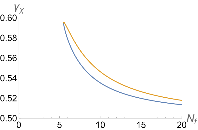
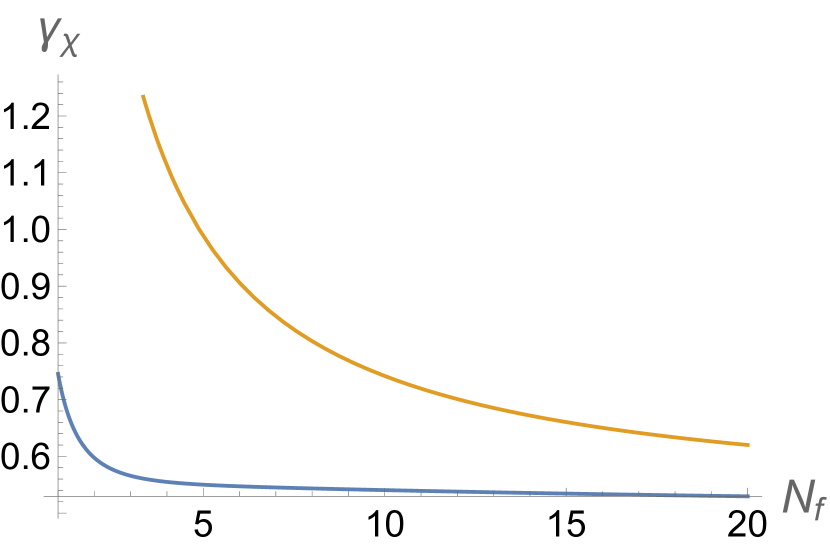
We spare the reader the expression for at two loops. The same physics applies also at this order: it is still true that there exists a unitary fixed point for all , and that at the fixed point is only unitary for . At large , still approaches the SUSY value regardless of . We present the results for in figure 1(a).
We can also perform the revised -expansion, where we set . In this case the fixed points are unitary for all , and again approaches the SUSY value at large . At one loop we have:
| (3.10) |
At two loops the results are presented in figure 1(b).
The results seem to suggest that we do not approach a SUSY fixed point for small , but that at large we may be approaching one. It is not clear that a two-loop analysis is enough in order to rule out SUSY at small , since the 1-loop and 2-loop contributions to the anomalous dimensions are of the same order of magnitude, and so the two-loop expansion does not seem like a good approximation. It is possible that our approximation is only valid at large- where additional contributions are suppressed, which would indicate that a SUSY fixed point is indeed reached.
3.3 Mesons
In this section we analyze the anomalous dimensions of meson operators. We will focus on two types of mesons operators:
| (3.11) |
with a flavor index and the auxiliary index. We are interested in their one-loop anomalous dimensions.
To compute e.g. the anomalous dimension of the scalar meson , we compute the three-point correlator
| (3.12) |
While the correlator itself is gauge-dependent, the anomalous dimension of the meson is not. Thus, we can compute in a specific gauge, and then apply the result for the latter independently of the gauge. In the -expansion, the one-loop result will take the form
| (3.13) |
where
| (3.14) |
Here the first term in the brackets is the tree-level contribution, and the second term is the diverging part of the one-loop result (and we ignore non-diverging terms). The anomalous dimension is then given by
| (3.15) |
where is the scalar wavefunction renormalization, which we recover from the anomalous dimension found in Luo:2002ti . In principle we would now have to diagonalize the anomalous dimension matrix, but in practice the diagonalization is immediate since we know there should be an adjoint and a singlet meson, which we denote by and . For the scalar and mixed mesons, the dimension is then given by
| (3.16) | |||
| (3.17) |
and similarly for . If in we recover SQED, we expect to find
| (3.18) |
We now present the results, with the details appearing in appendix A. For general and , the 1-loop anomalous dimensions are:
| (3.19) | ||||
| (3.20) | ||||
| (3.21) |
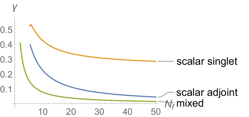
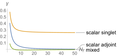
In the standard -expansion, the results for appear in figure 2. Again, the fixed points are non-unitary for small and so the anomalous dimensions are complex, but become real for large enough . At large , at the fixed point , all anomalous dimensions behave as , and so at large our results are consistent with a SUSY fixed point, since the anomalous dimensions of scalar and mixed mesons in both representations are equal. This is also in agreement with the results of the large expansion done in Benvenuti:2019 . On the other hand, at the fixed point with , at large the anomalous dimension of the singlet contraction of tends to a finite number, while the rest are . We thus conclude that only the fixed point with can lead to SUSY in at large .
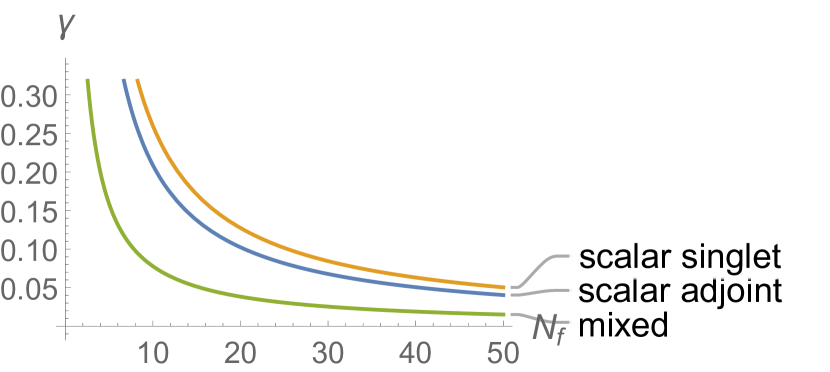
The results for the revised -expansion appear in figure 3. Only the fixed point with leads to a perturbatively stable theory. At small we do have a unitary fixed point, but it does not look like a SUSY fixed point. In particular for we find
| (3.22) |
At large SUSY is violated since approaches while approaches . We conclude that the revised -expansion fails to lead to SUSY in .
In order to perform yet another check to see whether we approach SQED fixed point for the specific value of , one can also use the proposed duality to the WZ model discussed in section 2.1. The duality maps mesons to specific operators in the WZ model and by comparing our results to those obtained in the -expansion for the WZ model we can see whether we approach the expected result. In agreement with the results above which indicate that we do not approach a SUSY fixed point for small , our results are far from the expected anomalous dimensions that the duality proposes in both the standard -expansion (where the fixed point isn’t unitary) and the revised -expansion.
Acknowledgements
The authors would like to thank O. Aharony for many helpful discussions and for comments on a draft, and thank I. Klebanov for comments on a draft. This work was supported in part by Israel Science Foundation grant no. 2159/22, by Simons Foundation grant 994296 (Simons Collaboration on Confinement and QCD Strings), by the Minerva foundation with funding from the Federal German Ministry for Education and Research, by the German Research Foundation through a German-Israeli Project Cooperation (DIP) grant "Holography and the Swampland", and by a research grant from Martin Eisenstein.
Appendix A Meson calculations
We compute the anomalous dimensions of mesonic operators using a direct computation of correlation functions. The simplest correlation function to consider for the scalar mesons is , which is understood to be in terms of bare operators. The relation to renormalized operators is:
| (A.1) |
The convention for renormalization of fields is and similarly for other operators. This is different compared to the convention of e.g. Luo:2002ti (where the fields are renormalized by ).
The factors are chosen according to the MS scheme. We can deduct the scalar renormalization, which for equals (in gauge):
| (A.2) |
Then, the anomalous dimensions of the meson operator can be derived via the relation
| (A.3) |
with the renormalization scale. The diagrams we need to compute are shown in figure 4. There are additional diagrams, contributing to the external leg corrections. However, we can infer their sum from , which we derive from its relation to , which in turn we can compute from the formulas in Luo:2002ti .
We can thus extract the renormalization function:
| (A.4) |
This expression should be viewed as an matrix, with the indices indicating the row and indicating the column. When we order the index multiple first by and then by , and the columns first by and then by , the renormalization matrix is of the form:
| (A.5) |
with the identity matrix, and . The eigenvalues of this matrix are with a multiplicity of and with a multiplicity of . These correspond to the adjoint and singlet representations appearing in the product , respectively. The anomalous dimensions are then:
| (A.6) | |||
| (A.7) |
We compute the anomalous dimensions of the mixed meson operators in a similar manner. We consider the correlation function . The only diagram that is not a propagator correction is shown in figure 5. The rest of the computation is completely analogous.
The anomalous dimensions all turn out to be:
| (A.8) |
Evaluating this for and general in the standard -expansion, we find
| (A.9) | ||||
| (A.10) | ||||
| (A.11) |
These are plotted in figure 2. At both fixed points , the anomalous dimensions of and tend to 0 as . However, only approaches 0 at the fixed point, whereas in the fixed point it approaches the finite limit . The results at the fixed point agree with SUSY and with Benvenuti:2019 . By contrast, the limit of at the fixed point deviates from them both.
We also show the anomalous dimensions of mesons in the revised -expansion in figure 3. Here, only the gives a perturbatively stable fixed point, and as in the standard -expansion. This is a violation of SUSY also in the large limit.
References
- (1) L. Fei, S. Giombi, I. R. Klebanov and G. Tarnopolsky, Yukawa CFTs and Emergent Supersymmetry, PTEP 2016 (2016) 12C105 [1607.05316].
- (2) S. Thomas, “Emergent Supersymmetry.” Seminar at KITP, 2005.
- (3) P. Liendo and J. Rong, Seeking SUSY fixed points in the 4 expansion, JHEP 12 (2021) 033 [2107.14515].
- (4) N. Zerf, L. N. Mihaila, P. Marquard, I. F. Herbut and M. M. Scherer, Four-loop critical exponents for the Gross-Neveu-Yukawa models, Phys. Rev. D 96 (2017) 096010 [1709.05057].
- (5) F. Benini and S. Benvenuti, = 1 QED in 2 + 1 dimensions: dualities and enhanced symmetries, JHEP 05 (2021) 176 [1804.05707].
- (6) F. Benini and S. Benvenuti, = 1 dualities in 2+1 dimensions, JHEP 11 (2018) 197 [1803.01784].
- (7) S. Prakash and S. Kumar Sinha, Emergent supersymmetry at large N, JHEP 01 (2024) 025 [2307.06841].
- (8) S. Jain, S. Minwalla and S. Yokoyama, Chern Simons duality with a fundamental boson and fermion, JHEP 11 (2013) 037 [1305.7235].
- (9) C. Choi, M. Roček and A. Sharon, Dualities and Phases of SQCD, JHEP 10 (2018) 105 [1808.02184].
- (10) D. Gaiotto, Z. Komargodski and J. Wu, Curious Aspects of Three-Dimensional SCFTs, JHEP 08 (2018) 004 [1804.02018].
- (11) A. Dey, I. Halder, S. Jain, S. Minwalla and N. Prabhakar, The large N phase diagram of = 2 SU(N) Chern-Simons theory with one fundamental chiral multiplet, JHEP 11 (2019) 113 [1904.07286].
- (12) J. Gomis, Z. Komargodski and N. Seiberg, Phases Of Adjoint QCD3 And Dualities, SciPost Phys. 5 (2018) 007 [1710.03258].
- (13) J. Eckhard, S. Schäfer-Nameki and J.-M. Wong, An 3d-3d Correspondence, JHEP 07 (2018) 052 [1804.02368].
- (14) V. Bashmakov, J. Gomis, Z. Komargodski and A. Sharon, Phases of theories in 2 + 1 dimensions, JHEP 07 (2018) 123 [1802.10130].
- (15) K. Inbasekar, S. Jain, S. Mazumdar, S. Minwalla, V. Umesh and S. Yokoyama, Unitarity, crossing symmetry and duality in the scattering of susy matter Chern-Simons theories, JHEP 10 (2015) 176 [1505.06571].
- (16) O. Aharony and A. Sharon, Large N renormalization group flows in 3d = 1 Chern-Simons-Matter theories, JHEP 07 (2019) 160 [1905.07146].
- (17) A. Sharon and T. Sheaffer, Full phase diagram of a UV completed = 1 Yang-Mills-Chern-Simons matter theory, JHEP 06 (2021) 186 [2010.14635].
- (18) G. Cuomo, L. Rastelli and A. Sharon, Moduli Spaces in CFT: Bootstrap Equation in a Perturbative Example, 2406.02679.
- (19) G. Cuomo, L. Rastelli and A. Sharon, Moduli Spaces in CFT: Large Charge Operators, 2406.19441.
- (20) W. Siegel, Supersymmetric Dimensional Regularization via Dimensional Reduction, Phys. Lett. B 84 (1979) 193.
- (21) S. Benvenuti and H. Khachatryan, Easy-Plane QED3’s in the large limit, JHEP 05 (2019) 214 [1902.05767].
- (22) M.-x. Luo, H.-w. Wang and Y. Xiao, Two loop renormalization group equations in general gauge field theories, Phys. Rev. D 67 (2003) 065019 [hep-ph/0211440].
- (23) S. J. Gates, M. T. Grisaru, M. Rocek and W. Siegel, Superspace Or One Thousand and One Lessons in Supersymmetry, vol. 58 of Frontiers in Physics. 1983, [hep-th/0108200].
- (24) M. Gremm and E. Katz, Mirror symmetry for N=1 QED in three-dimensions, JHEP 02 (2000) 008 [hep-th/9906020].
- (25) S. Gukov and D. Tong, D-brane probes of special holonomy manifolds, and dynamics of N = 1 three-dimensional gauge theories, JHEP 04 (2002) 050 [hep-th/0202126].
- (26) T. Appelquist and D. Nash, Critical behavior in (2+1)-dimensional qcd, Phys. Rev. Lett. 64 (1990) 721.
- (27) T. Appelquist, D. Nash and L. C. R. Wijewardhana, Critical behavior in (2+1)-dimensional qed, Phys. Rev. Lett. 60 (1988) 2575.
- (28) M. E. Machacek and M. T. Vaughn, Two Loop Renormalization Group Equations in a General Quantum Field Theory. 1. Wave Function Renormalization, Nucl. Phys. B 222 (1983) 83.
- (29) M. E. Machacek and M. T. Vaughn, Two Loop Renormalization Group Equations in a General Quantum Field Theory. 2. Yukawa Couplings, Nucl. Phys. B 236 (1984) 221.
- (30) M. E. Machacek and M. T. Vaughn, Two Loop Renormalization Group Equations in a General Quantum Field Theory. 3. Scalar Quartic Couplings, Nucl. Phys. B 249 (1985) 70.