Interplay between Majorana and Shiba states in a minimal Kitaev chain coupled to a superconductor
Abstract
Two semiconducting quantum dots (QDs) coupled through a superconductor constitute a minimal realisation of a Kitaev chain with Majorana zero modes (MZMs). Such MZMs can be detected by e.g., tunneling conductance between each QD and normal leads [Dvir et al, Nature 614, 445 (2023)]. We here discuss how the seemingly trivial substitution of one of the normal leads by a superconducting (SC) one gives rise to a plethora of new effects. In particular, the coupling to the SC lead induces non-local Majorana effects upon variations of the QDs’ energies. Furthermore, the lowest excitation of the chain is no longer determined by the bulk gap but rather by the energy of an emergent subgap Yu-Shiba-Rusinov (YSR) state coexisting with the MZMs. The YSR state hybridizes with the MZMs when the coupling between the SC and the QD is larger than the spin splitting, spoiling the Majorana properties, including the quantized conductance.
I Introduction
The Kitaev chain [1] is the minimal model for one-dimensional spinless p-wave superconductivity. In the topological phase, the chain hosts Majorana Zero Modes (MZMs) [2, 3, 4, 5, 6] at its ends, which feature non-abelian statistics that can be exploited for topological quantum information processing [7, 8, 9, 10]. New platforms based on arrays of quantum dots (QDs) connected through mesoscopic superconductors [11, 12, 13, 14] have emerged as a promising route toward bottom-up engineering of artificial Kitaev chains. This approach largely avoids undesired effects associated to disorder and material inhomogeneities inherent to other platforms [15, 16, 17].
A minimal Kitaev chain can be realized by just two QDs coupled through a mesoscopic superconductor that mediates crossed Andreev reflection (CAR) and elastic cotunneling (ECT) between the QDs [11, 12]. Such minimal Kitaev chains host “poor man’s Majorana states”, that share properties with their topological counterparts [18], but lack topological protection, since they appear at fine-tuned “sweet spots” in parameter space with equal CAR and ECT. Recent experiments have demonstrated exquisite control on CAR and ECT amplitudes [19, 20, 21, 22], which allows to tune sweet spots [23, 24, 22, 25, 26] where one MZM localizes in each QD of the minimal chain. Interestingly, longer chains, already at the three QD level, start to show a bulk gap and some degree of protection [26].
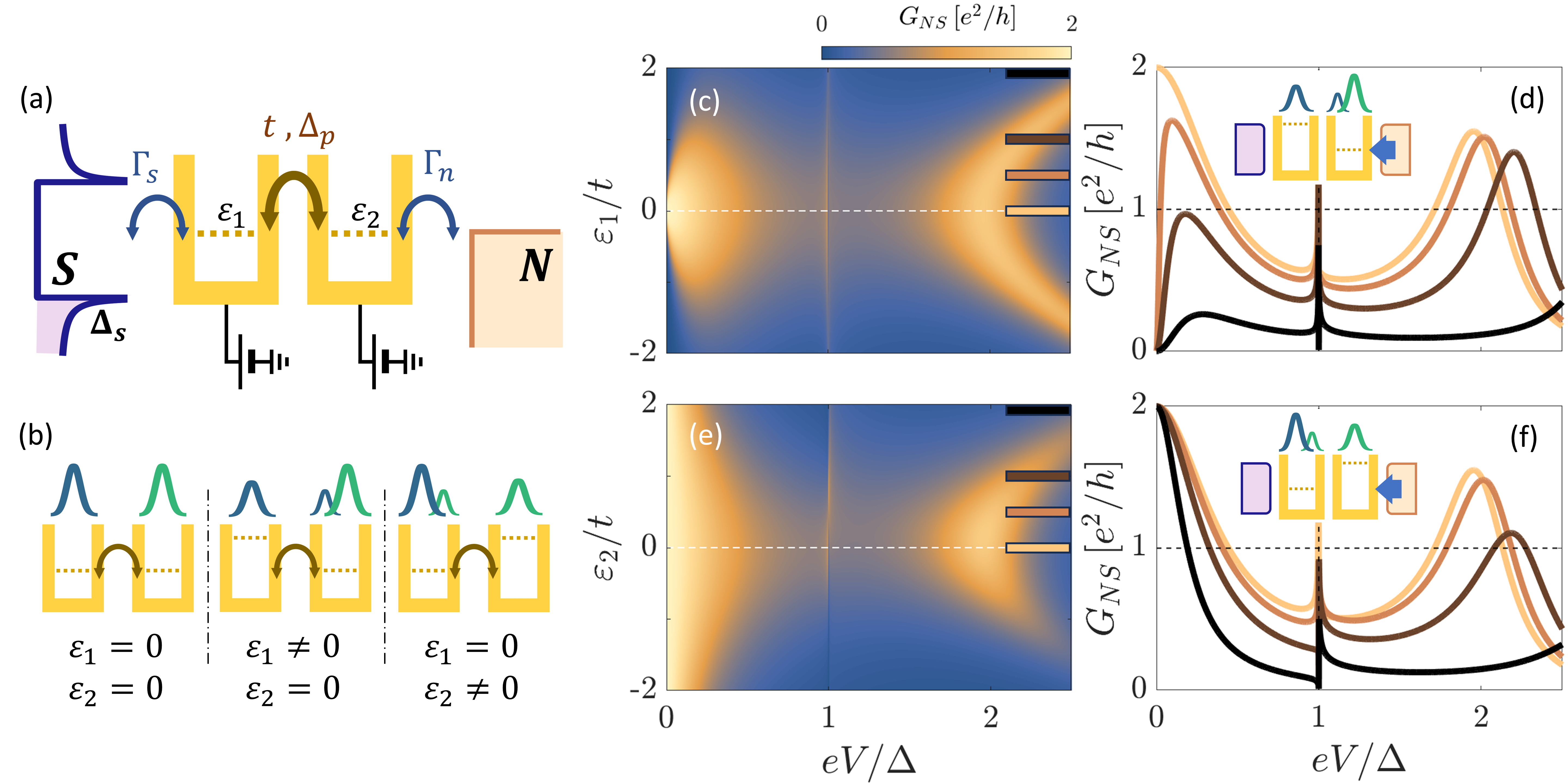
So far, the assessment of sweet spots has been done via local and non-local normal conductance, by coupling the system to metallic leads [19, 20, 21, 24, 22, 25, 26]. In this work, we explore what happens beyond this minimal setup and theoretically study the transport properties of a minimal Kitaev chain coupled to a normal and a superconducting (SC) probe, see Fig.1(a), inspired by recent experimental configurations, Refs. 22, 26.
One consequence of the replacement of one of the normal leads by a SC one, is the change of the the well-known quantized zero bias peak [27, 28, 29], which now becomes when the BCS coherence peak aligns with the MZM [30, 31]. Despite the lack of topological protection in this minimal setup, we find a less obvious result: the universal conductance values through either the normal or the SC probe are robust against local detuning of the QD in contact with such probe. Further analysis in this work includes a detailed study of the role of the asymmetries and non-local effects induced by the inclusion of the non-trivial self-energy associated to the SC lead. As we discuss, this phenomenology could be used as a way to measure the degree of localization [32] of the MZMs in the minimal Kitaev chain and to characterize sweet spots.
Interestingly, the regime of strong hybridization between the SC and the minimal Kitaev chain is governed by the emergence of Yu-Shiba-Rusinov (YSR) states [33, 34, 35, 36, 37, 38]. The interplay between MZMs and YSR has already been studied previously using minimal models neglecting the continuum of quasiparticles above the SC lead [39, 40]. Their inclusion, however, results in important physical consequences since the energy of the YSR states decreases when increasing the coupling to the lead, thus reducing the effective gap between MZMs and the excited states. A finite spin-polarization in the dots generates a destructive interference between the YSR states and the MZMs which spoils the topological properties of the latter, including the conductance quantization. In the language of non-Hermitian open quantum systems, we understand the topological properties of the hybrid junction in terms of Exceptional Point (EP) bifurcations in the subgap spectrum [41, 42, 43, 44, 45], characterized by a change of the MZMs localization.
The rest of the manuscript is organized as follows: in Sec. II we introduce the effective minimal model to describe the system, giving some analytical insights on the renormalization of the excited state by means of the coupling to the SC lead.
In Sec. III and IV we study both, the normal and superconducting conductance when detuning both QDs in the weak and strong coupling regime with the SC lead respectively. Sec. V is devoted to the analysis of the coexistence of MZMs and YSR states, referring to spectral properties such the localization of the states and the pole structure of the system. We extend this analysis to the finite polarization case in Sec. VI, where the destructive interference between MZMs and YSR states spoils the Majorana properties for finite values of the coupling to the SC lead.
We finally offer, in Sec. VII, some conclusions summarizing the main results. Technical details like the explicit analysis of the poles of the system including the exceptional points, some notes on the Green functions used to compute both, spectral and transport properties and, the extension of the study of the physics associated to the QDs chemical potential to large couplings, are included in the appendices.
II Modelization
We examine a minimal Kitaev chain coupled to a normal and a SC leads, as sketched in Fig.1(a). We consider that the system is subject to a strong magnetic field that fully polarizes the quantum dots spins. The two QDs are coupled via a central SC, that mediates ECT and CAR, with effective amplitudes and respectively, realizing a one dimensional spinless p-wave SC that can host MZMs [11]. External gates can be used to tune the chemical potential on the two QDs independently ( and ), changing the degree of localization of the MZMs, see Fig.1(b). The minimal Kitaev chain is coupled to the SC (normal) lead through the tunneling rate (), being () the coupling and () the bandwidth.
To describe the transport properties of the device, we use the non-equilibrium Green’s function formalism [46, 31, 47, 48, 49], that allows us to consider arbitrary coupling strengths between the minimal Kitaev chain and the leads, see Appendix D and F for details. In addition, the poles of the Green’s function determine the energy of the system’s states that can be related to the main transport features. Notice that for a spin-polarized chain, there is no subgap Andreev reflections with the SC probe [50] due to the incompatibility between order parameters across the junction [51, 30, 31] (i.e., a BCS lead with s-wave pairing and a spinless SC with p-wave pairing [52]).
In the sweet spot (i.e., and ) and limit, the poles of the Green function are contained in the characteristic polynomial
| (1) | |||||
Along with the zero-energy poles, there appears other subgap structure that may describe the excited states () in certain parameter regimes. The non-perturbative coupling to the SC lead renormalizes the energy of such excited states, appearing as subgap poles detaching from the continuum. These poles can be obtained analytically (cf. App. A for details), and we reproduce here an approximation to the lowest contribution in
| (2) |
where , and .
III Weak coupling
We first examine transport through the normal lead when the Kitaev chain is weakly coupled to the SC lead (), comparing it to the previously known phenomenology [11, 24].
Figure 1(b) illustrates the Majorana localization when detuning the two QDs away from the sweet spot. When QD1 is detuned, the two MZMs have a finite spectral weight in QD2. Thus, when considering , the normal lead couples to both MZMs, producing a destructive interference sharp dip at zero energy, Fig.1(c), as previously observed in Ref. 11. Moreover, due to electrons tunneling between the normal and the SC lead, mediated by the Kitaev chain, a peak appears at , where , see also Fig.1(d).
By contrast, when QD2 is detuned from the sweet spot, the two MZMs acquire a finite weight in QD1. This leads to a quantized zero-bias conductance peak, showing a width that depends on , cf. Fig.1(f) and Ref. 11. Therefore, detuning either the QD attached to the normal lead or the one attached to the SC lead has very different effects on the transport properties.
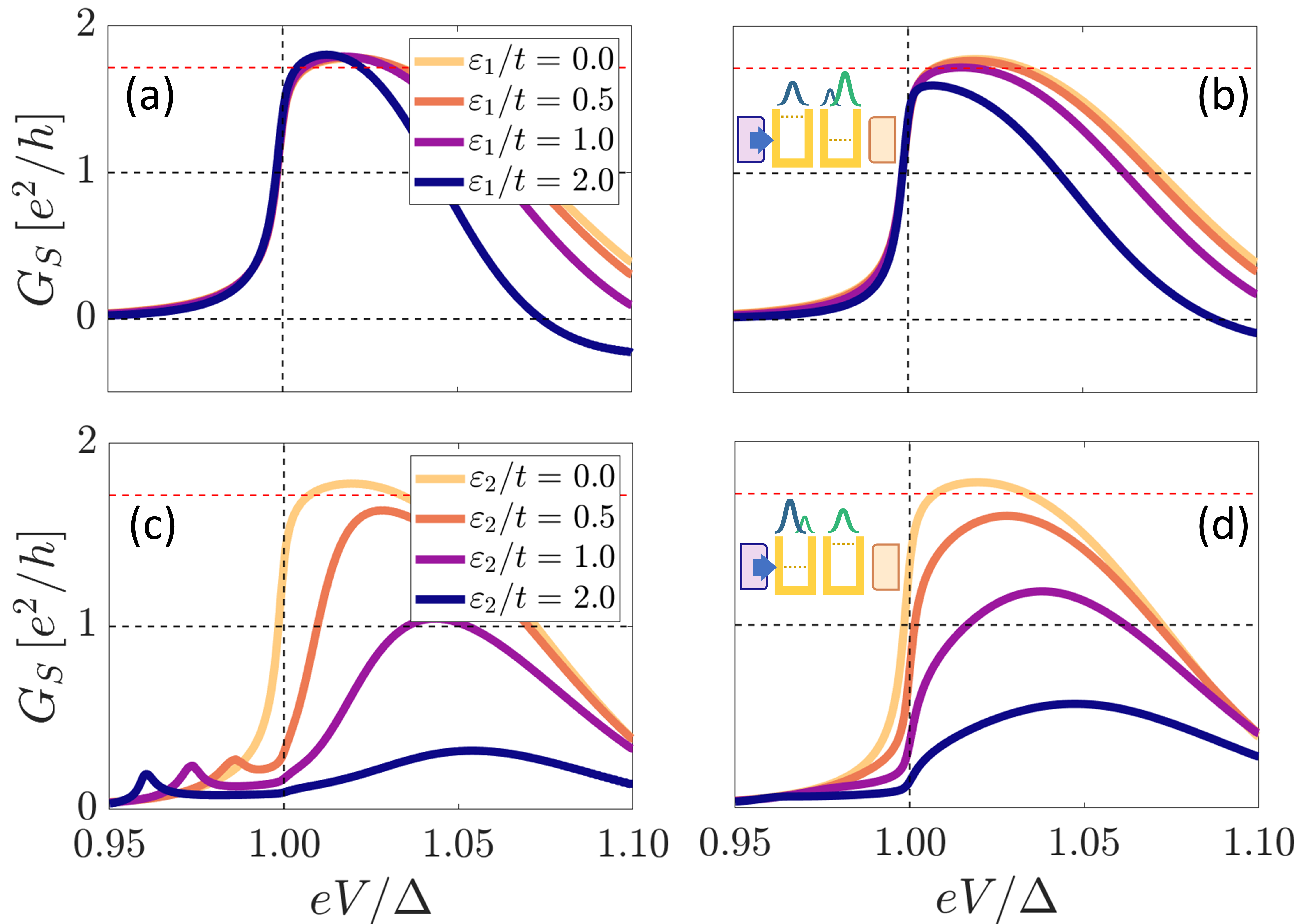
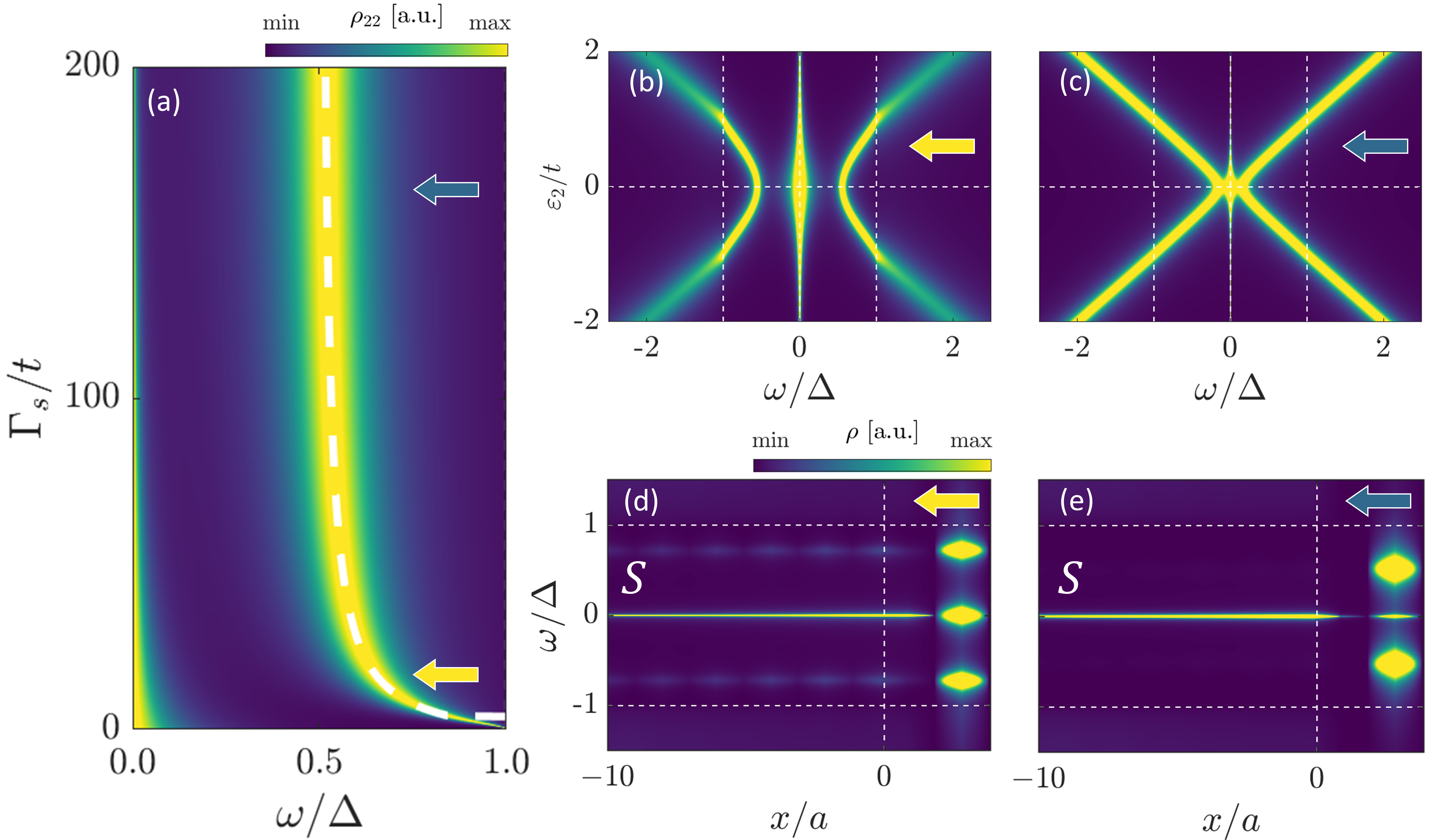
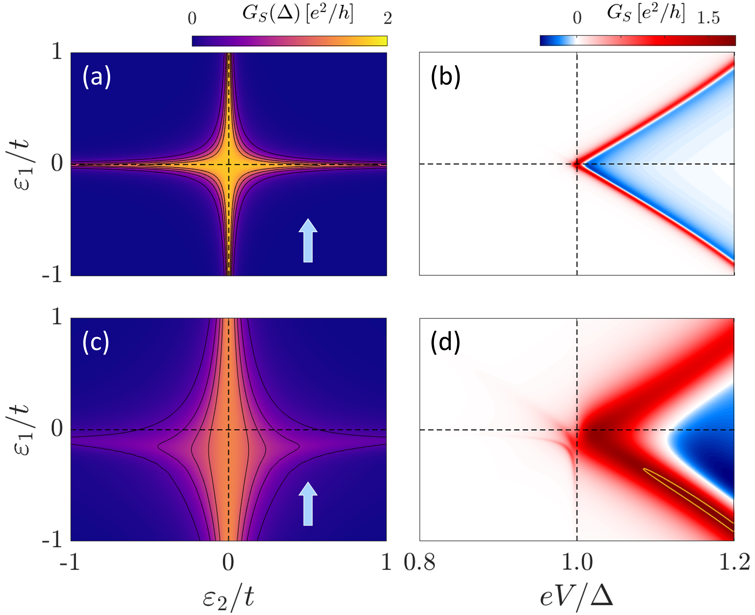
We now systematically analyze the role of level detuning in SC transport in the regime of weak coupling to the normal lead (), see Fig. 2. Specifically, we concentrate on the features close to the gap, as subgap transport is suppressed due to the QD spin-polarization. Figures 2(a,b) show how SC transport is locally modified as the QD directly coupled to the SC lead is detuned, therefore pushing the MZM spectral weight to the opposite QD. The conductance measured in the SC exhibits an approximately quantized value, at , almost independently of the value of , thus reproducing the phenomenology predicted for nanowires [30, 31], see Fig.2(a). However, a small reduction in the conductance height at can be seen for larger values of and , see Fig.2(b).
Figure 2(c,d) illustrates the opposite behaviour, namely how SC transport is modified non-locally when the QD far from the SC lead is detuned. In this case, the lead couples to both MZMs. The resulting hybridization becomes evident when testing transport through the SC probe, where the quantized conductance value gets reduced as soon as . Moreover, the coherent coupling between MZMs mediated by the SC lead, gives rise to subgap signatures in transport, Fig. 2(c). We remark that the subgap structure is not associated to any renormalization of subgap poles but to inelastic single-particle processes in transport, cf. Refs. [53] and App. D. When the coupling to the normal lead is increased, the spreading of the MZM into the normal lead enhances the SC transport, Fig. 2(d). Notice that this dependence with is the opposite to the one found in the case in Fig. 2(a, b).
IV Strong coupling
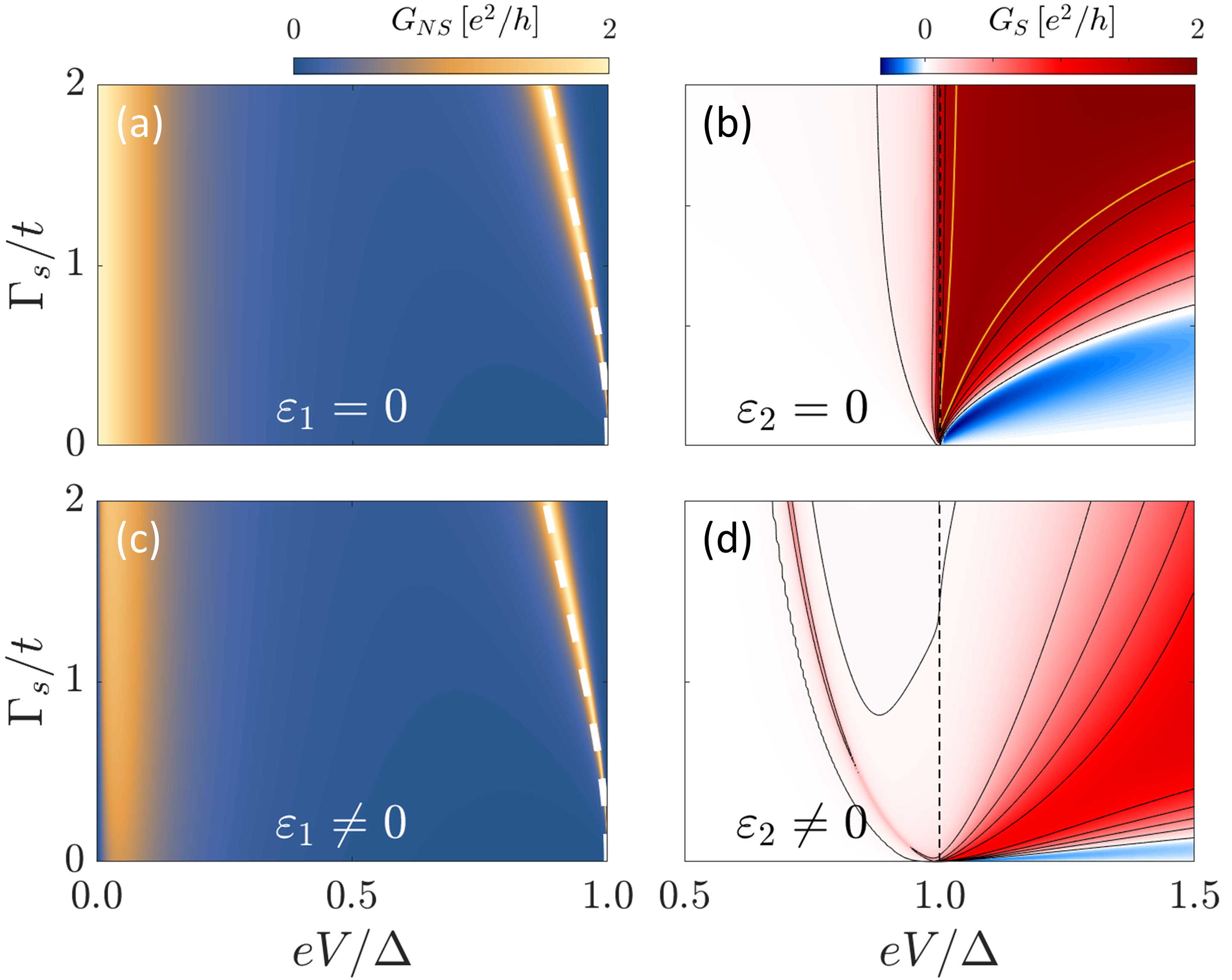
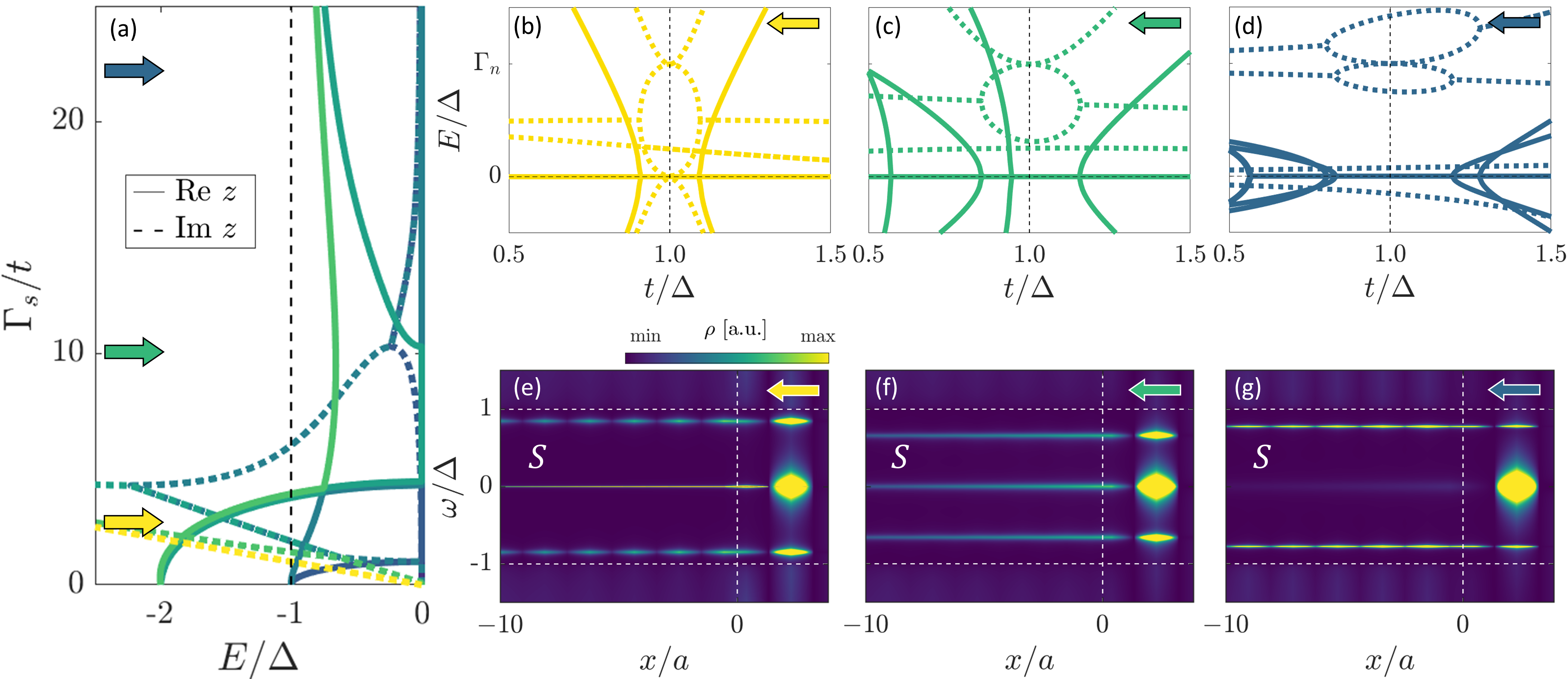
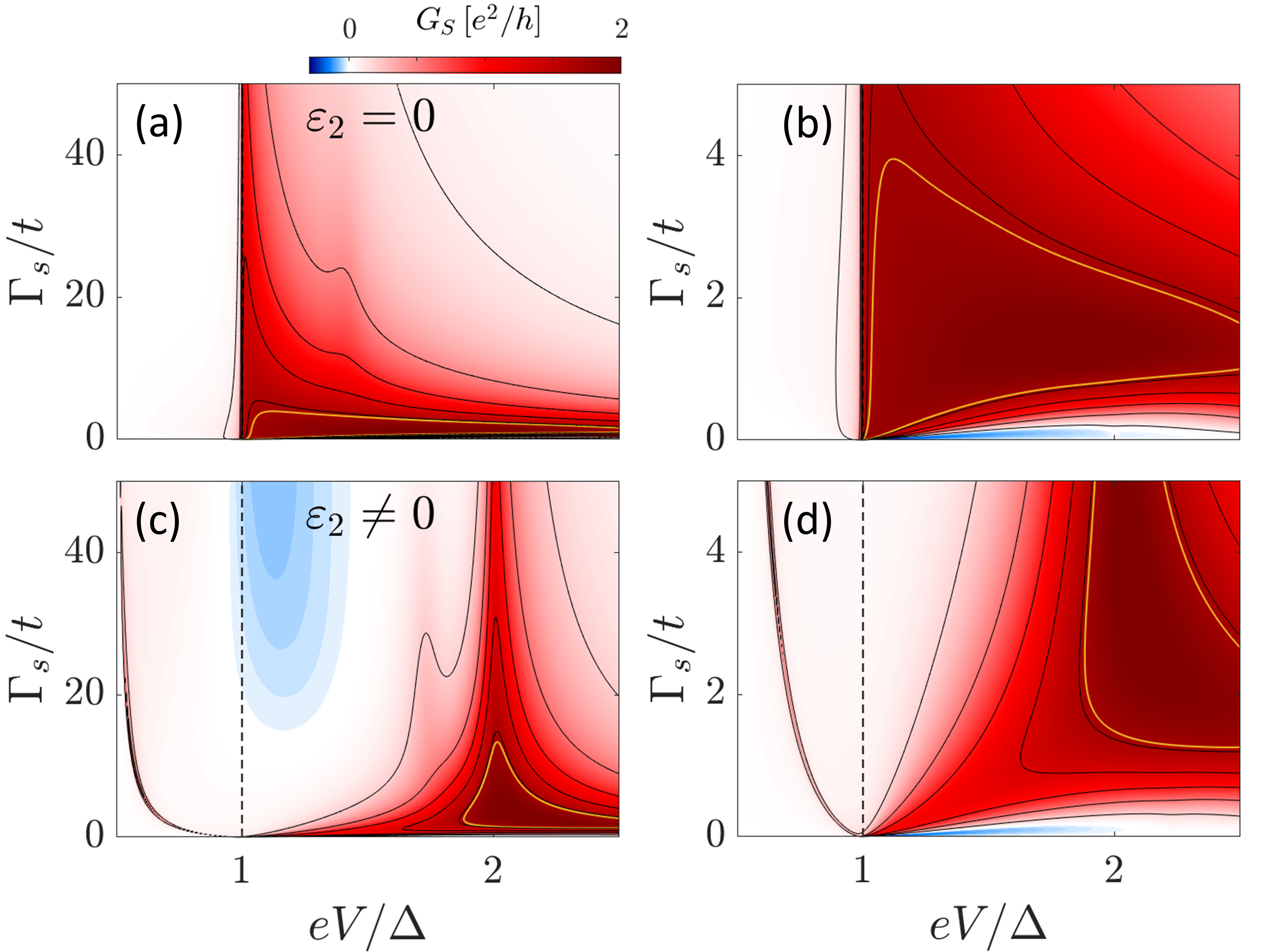
Now we examine the electron transport as a function of the coupling to the SC lead, going beyond the weak coupling regime () where the excited state at is strongly renormalized by the lead, emerging as a subgap YSR state [53, 54, 55, 56, 39, 40]. Transport provides an ideal method to observe the interplay between the aforementioned YSR states and MZMs, Fig. 3. The onset of the YSR state appears as a new peak detaching from the continuum with linear dispersion around , Figs. 3(a, c). This phenomenology does not affect the MZM signatures at , except for and finite spin-polarization in QD1, see below and App. C. The conductance of the excited state is also quantized for and . Intuitively, the excited state is no longer broadened by the SC lead when is well detached from the continuum, thus recovering the Majorana properties of the original excited state.
Detuning barely affects the excited state and only leads to a dip in the zero-bias conductance, as commented in the weak coupling regime, see Fig. 1. The energy of the excited state is renormalized when shifts away from the sweet spot, losing any quantized behaviour in transport. In particular, it gets pinned to for large values, cf. App. A.
Transport through the SC lead is also affected when increases, Fig. 3(b, d). First, the universal height value moves to larger values of the voltage bias as the coupling to the SC lead is increased [53], illustrated by the yellow line. Figure 3(d) shows the onset of a subgap structure associated to the hybridization between Majoranas when detuning QD2 even in the weak coupling regime , see also Fig. 2(c). This subgap structure is obtained from the single-particle contribution when testing transport through the SC probe when enabling thermally activated inelastic cotunneling, Thus, the hybridized MZMs behaves as a trivial zero energy subgap state in the strong tunneling regime [53], cf. App. D and E. Notice that the conductance peaks have a reduced value, compared to panel (b) and for the dispersion of the subgap peak is linear with (i.e., quadratic with ) highlighting the different origin with the observed subgap structure in Fig. 3(a,c).
V Interplay between YSR and MZMs
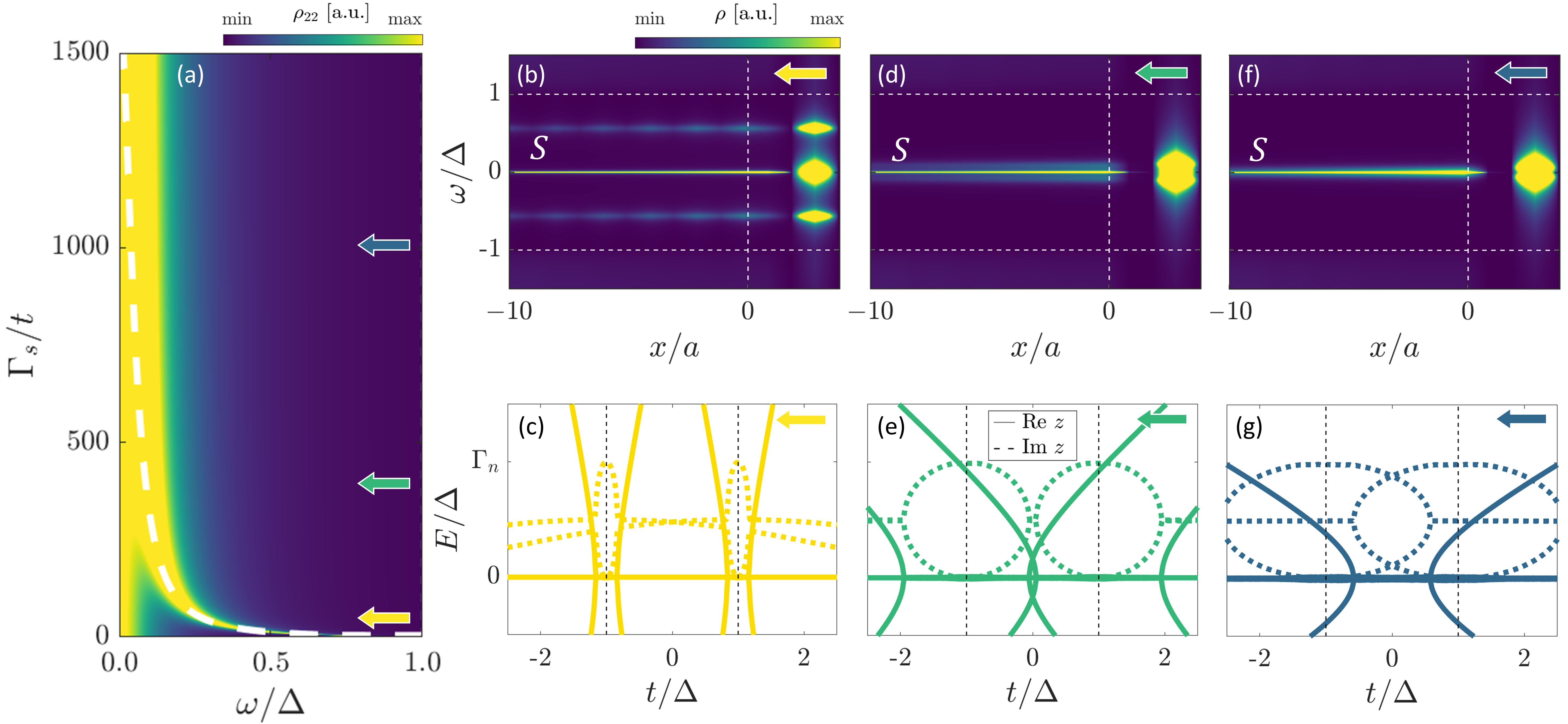
The previous transport characteristics can be understood in terms of the Local Density of States (LDOS) which provides a way to study the transition from the weak to strong coupling to the leads (), resolving the degree of localization of the different subgap states, cf. App. B.
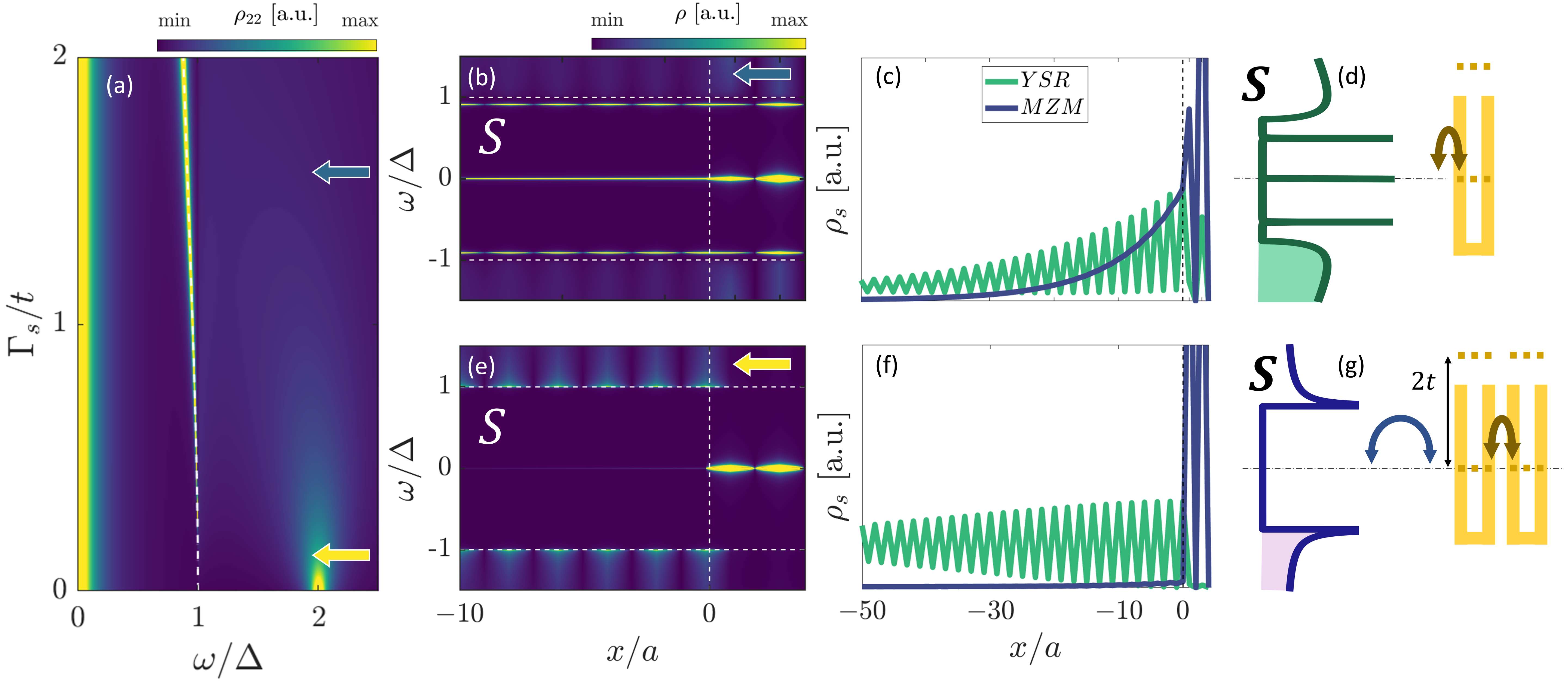
The LDOS at QD2, Fig. 4(a), features a transition around in which the excited state at disappears and re-appears as a subgap state The transition also reflects on a different localization of the states in the weak and strong coupling regimes, see Figs. 4(b,e). For weak coupling to the SC (), the system hosts confined MZMs where the SC lead acts as a gapped lead, Fig. 4(f). Therefore, we characterize this regime as a minimal Kitaev chain, where the excited states are just broadened by the coupling to the leads, see Fig. 4(g). In contrast, in the strong coupling regime , both the MZM and the subgap state at , extend into the SC lead, Fig. 4(b, c). In this limit, the SC lead + QD1 system is described by a YSR-like state, where QD1 is subsumed in the SC lead, see Fig. 4(d). The coupling between the YSR state and QD2 renormalizes the excited state, reducing its energy while the MZM remains at . In this limit, the correct physical picture is no longer that of a minimal Kitaev chain weakly coupled to both SC and normal leads, but rather of a YSR coexisting with a MZM.
The energy of these YSR states decreases as increases, merging with the MZMs at zero energy for for a fully spin-polarized QD1. A non-zero allows for the merging to occur at a finite value of the coupling with the SC lead, making it hard to demonstrate the Majorana properties of the chain as the gap to excited states goes to zero [43], see Fig. 5(a). The dashed line shows the convergence of the YSR state to zero energy, described by Eq. (1), and the width of the state is determined by . Even though the YSR and the Majorana states overlap, the zero-bias conductance quantization is preserved (not shown).
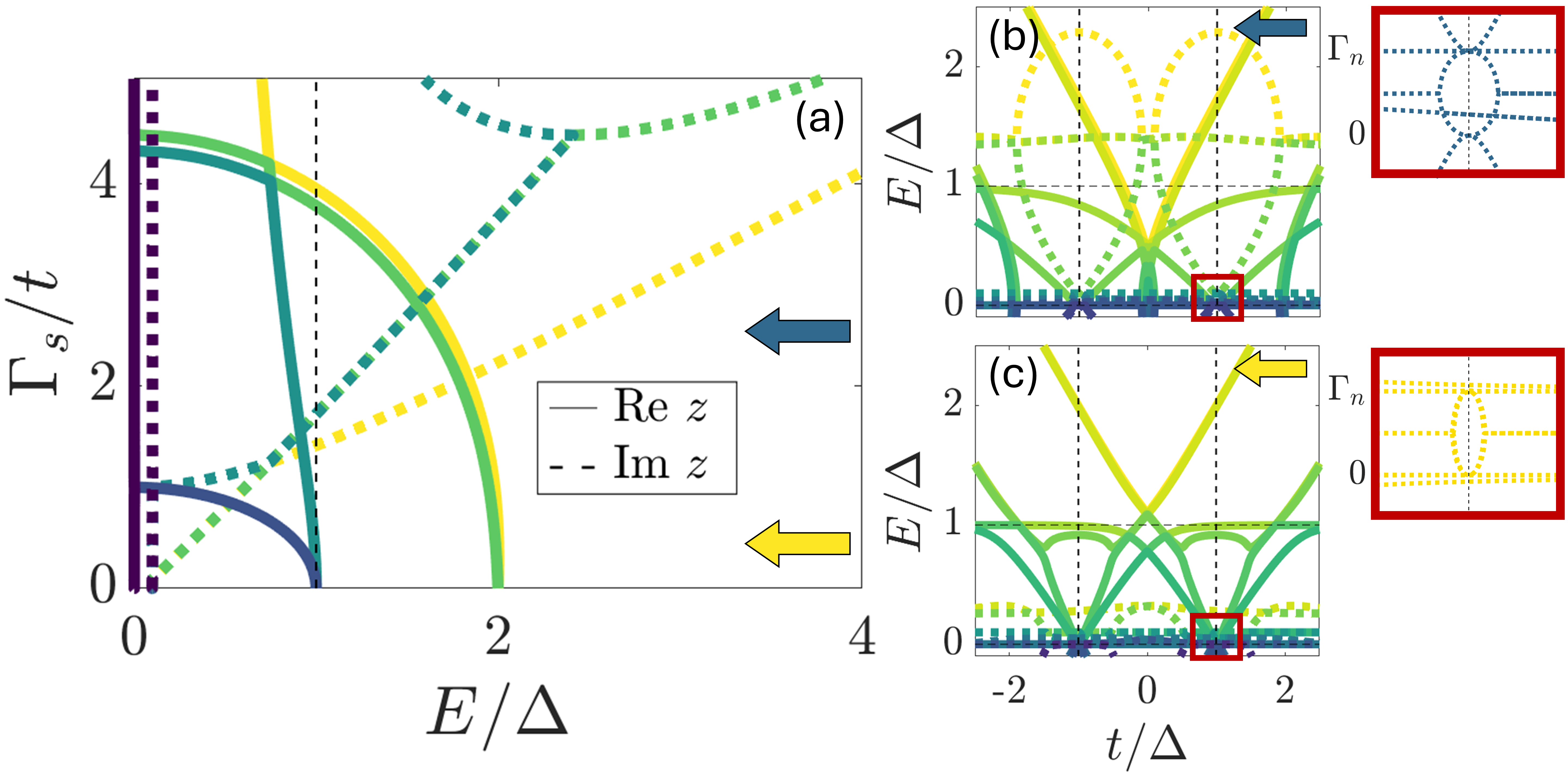
The merging of the YSR and the MZM states can be understood in terms of the LDOS across the junction and the EP associated to the zero poles, i.e., non-Hermitian spectral degeneracies in the complex spectrum of the system when considering the strong coupling to the leads. This EPs are seen as bifurcations in the poles’ imaginary part where eigenvalues and eigenvectors coalesce [41]. For , along with the EPs associated to the MZM, new secondary EPs appear linked to the quantized conductance behaviour of the YSR excited state in this regime, cf. App. A. Moreover, we observe a new regime at such there is a transition of the pole defining the dispersion of the YSR state, see also Fig. S 1 in App. A. Furthermore, in this regime the MZM at QD1 is being absorbed by the SC lead, Fig. 5(b).
For larger values of the coupling, the EPs centered around start to touch each other, signalling the overlap of the subgap states, see Fig. 5(c,e). The spectral weight at zero energy in QD1 is suppressed as the MZM is delocalized into the lead, Fig. 5(d). For even larger values of the coupling, the EPs intersects and the extended MZM living in the SC lead becomes narrower and narrower, Fig. 5(f,g). Thus, we observe a non-destructive overlap between the YSR and MZMs that preserve a confined zero energy subgap state with quantized conductance.

VI Finite spin-polarization
In real experiments, the QDs have a finite spin polarization. Despite both QDs being subjected to the same global magnetic field, a strong coupling to the SC will strongly renormalize the g-factor of QD1 [39]. To account for this effect, we consider a finite Zeeman splitting in QD1 () while keeping QD2 spin-polarized, although our findings remain qualitatively invariant for a finite spin-splitting in QD2.
Due to the partial polarization in QD1, the coupling with the SC lead is able to mix spin up and down, leading to a competition between the Zeeman splitting and the hybridization with the SC. This competition reflects in the density of states as an avoided crossing between the MZMs and the YSR states, see Fig. 6(a). After the maximum approaching, the Majorana properties are spoiled, including the quantized zero-bias conductance, see Fig. 6(b). The transition happens for . Moreover, when the YSR state is well detached from the continuum, it exhibits quantized conductance behaviour and coupling dependent width. However, this quantized regime is reached when the ZBP is completely lost, as a signature of the destructive interference in contrast to the fully spin-polarized case.
Figure 6(c,d) reflect that as the Zeeman field in QD1 increases, the crossing point is displaced to larger values of the coupling to the SC lead in such a way that for full polarization, the regime of destructive interference is never reached and the gap to the excited state reduces with [40]. Therefore, in the ultra-strong coupling regime, the degree of polarization is relevant to the physics of the problem. In this regime MZMs are present only for . Thus, it is important to preserve a well-defined spin-polarization of the YSR state along with including the effects of the continuum of quasiparticles when considering Kitaev chains formed by ABS-QDs building blocks [39, 40].
VII Conclusions and Outlook
Artificial Kitaev chains made out of quantum dots (QDs) coupled to superconductors (SCs) have emerged as promising platforms to probe Majorana physics. In this work, we have demonstrated that a SC can be used to probe the properties of Majorana states appearing in minimal Kitaev chains, offering insights about their localization. This reflects in non-local subgap features in the SC conductance when the chemical potential of the QD far from the SC lead is detuned.
We have characterized the weak and strong coupling to the SC lead as the evolution from a minimal Kitaev chain, to a system defined by the coexistence of a YSR state and MZMs. The energy, and therefore the gap to the excited state, decreases with the coupling to the SC. For finite spin-polarization in the QDs, the coupling to the SC induces a YSR-Majorana hybridization, spoiling the characteristic properties of the Majorana states, including the conductance quantization. This illustrates the competition between YSR and Majorana physics in minimal Kitaev chains.
We foresee the extension of the analysis to hybrid setups where one could induce transport through an Andreev bound states, e.g. by including an extra QD between the SC lead and the minimal Kitaev chain, leading to extra resolution of subgap features.
Acknowledgements.
We thank A. Bordin and M. Pino for valuable comments and discussions. Work supported by the Horizon Europe Framework Program of the European Commission through the European Innovation Council Pathfinder Grant No. 101115315 (QuKiT), the Spanish Comunidad de Madrid (CM) “Talento Program” (Project No. 2022-T1/IND-24070), the Spanish Ministry of Science, innovation, and Universities through Grants PID2022-140552NA-I00, PID2021-125343NB-I00 and TED2021-130292B-C43 funded by MCIN/AEI/10.13039/501100011033, “ERDF A way of making Europe” and European Union Next Generation EU/PRTR. Support from the CSIC Interdisciplinary Thematic Platform (PTI+) on Quantum Technologies (PTI-QTEP+) is also acknowledged.Appendix A Poles Structure and EPs
In the main text, we have described a hybrid setup consisting in a quantum dot (QD) based minimal Kitaev chain coupled to a normal and a superconducting (SC) lead which can be described by the boundary Green’s functions (bGF) [46, 31, 47, 48, 49] written in the (hat notation) Nambu basis
| (3) |
where () are Pauli matrices acting in spin (electron/hole) space, both in the wide-band approximation . The coupling terms between the different elements across the junction take the form and, the toy model for the minimal Kitaev chain [11] in this basis,
| (4) |
where are the projectors over the spin up/down sector. Notice that as one reaches the polarized limit of the minimal Kitaev chain when , the coupling between the QDs in the spin down sector goes correspondingly to zero. It should be reminded that the effective coupling between QDs is obtained from a Schrieffer–Wolff transformation and therefore, it is inversely proportional to the energy difference between states. Thus, the GFs projected over the minimal Kitaev chain can be computed working directly on a spinless basis , equivalent to remove the anomalous part of the SC lead’s GF in the calculation. This effect is associated to the incompatibility between order parameters between the SC lead and the Kitaev chain. Unless otherwise stated, we use and . In the spin-less basis it is satisfied that
| (5) |
and the total GF projected over the QDs takes the form
| (6a) | ||||
| (6b) | ||||
where the bGF associated to both ends of the minimal Kitaev are
| (7a) | ||||
| (7b) | ||||
and
| (8a) | ||||
| (8b) | ||||
Without any loss of generality, the poles of the system (shared by both QDs) can be obtained from in Eq. (6). Then, the associated self energy due to the coupling to QD2 including the adjacent normal lead , simplifies to
| (9) |
where describes the poles associated to the QD2 coupled to the normal lead, being the hybridization parameter with the normal lead.
Finally, the analytical expression for can be written as
| (10) |
where
| (11) |
and , where is the hybridization with the SC lead. Notice that the characteristic polynomial has 16th degree in and contains all the information concerning the poles of the system. In the sweet spot and limit, the polynomial simplifies to
| (12) |
Along with the zero modes, there are other subgap poles that can be computed analytically as
| (13a) | ||||
| (13b) | ||||
| (13c) | ||||
where the parameter can be either or . Depending on the parameter regime, the excited state of the system () may be described by one of these subgap poles.
Figure S 1 shows the real and imaginary parts of the poles of the system including non-Hermitian effects such . Thus, we are able to study the Exceptional Points (EPs) [42, 43, 44, 45] for different values of the coupling to the SC lead. Figure S 1(a) shows several transitions where the real part of some poles goes to zero. First, a transition at appears as one of the poles detaching from the continuum goes to zero (i.e., ), defining the change of regime from weak to strong coupling.
In the weak coupling limit, there are only EPs associated to the Majorana Zero Modes (MZMs), where the excited state can be found at . Figure S 1(c) illustrates the EPs associated to the imaginary part of the zero poles in this regime. The maximum (minimum) value of the bifurcation at the sweet spot is () signaling that one of the Majorana poles is non-decaying and completely decoupled from the leads [42, 44] (i.e., there is no effective coupling with the SC lead in the weak coupling owing to the SC gap).
Above the transition, the excited state behaves as a Yu-Shiba-Rusinov (YSR) state defined by the subgap pole in Eq. (13a). Remarkably, in this regime appears other secondary EPs coexisting with the main one, see Fig. S 1(b). These secondary EPs can be related to the quantized transport behaviour of the YSR in the normal conductance mentioned in the main text. The maximum (minimum) value of the bifurcation at the sweet spot is (), signalling a configuration with maximum coupling asymmetry [42].
Finally, Fig. S 1(a) shows another transition when around , where a bifurcation of the imaginary parts of the poles take place defining the ultra-strong coupling regime. Above this transition, the excited state is described by in Eq. (13a). Finally, in the limit the YSR state merges with the MZMs. However, when detuning QD2 the ultra-strong coupling regime physics are strongly renormalized.
Figure S 2 illustrates the associated physics when detuning QD2. The excited states obeys that when then . More in particular, when , the excited state is defined by a renormalized YSR state that do not merge with the MZMs, see Fig. S 2(a). Fig. S 2(d,e) shows that in the ultra strong coupling regime, the excited subgap state becomes strongly localized at QD2. Moreover, there is no longer secondary EPs for large couplings, which can be related to the lack of a quantized transport response, leading to a vanishing normal transport signal in the ultra-strong coupling regime (not shown). By contrast, when , the excited state becomes pinned to even at the strong coupling transition .
Analyzing the dispersion of the excited state with ,, for moderate couplings the excited state follows a parabolic dispersion, Fig. S 2(b). However, as the coupling with the SC lead is increased, the minimum of the parabola is displaced to smaller energy values and the dispersion is slightly renormalized. In the limit , the excited state becomes linear with , and the energy minimum finally collapses to zero, see Fig. S 2(c). By contrast, when detuning QD1, the parabolic dispersion of the excited state with becomes constant, as QD1 is being absorbed by the SC lead for large couplings (not shown).
Appendix B Penetration of subgap states
We follow Ref. 48 to analyze the penetration of the subgap poles into the leads from the total advanced GF to compute the Local Density of States (LDOS) as in the Nambu basis, where the GF in the semi-infinite SC lead acquires the form
| (14) |
where is an integer position index running into the left SC lead and being the coupling between neighbouring sites inside the SC lead. The GFs associated to the isolated semi-infinite SC lead takes the expression
| (15a) | ||||
| (15b) | ||||
| (15c) | ||||
Finally, the translationally invariant GFs associated to the SC bulk are defined by
| (16a) | ||||
| (16b) | ||||
| (16c) | ||||
It should be noticed that to obtain a proper convergence of the GFs across the SC lead, is defined out of the wide-band approximation, i.e., the normal and anomalous part of the bGF are
| (17a) | ||||
| (17b) | ||||
It is trivial to see that, to compute the penetration into the normal lead, one has to transform the previous expressions following where , , and . The normal bGF can be obtained from Eq. (17a) considering , where , and for advanced GFs.
Appendix C Finite spin-polarization on QD1
In the main text we have discussed a configuration where QD1 acquires a finite spin polarization, leading to the coexistence of the YSR and MZMs occurring at much smaller couplings with the SC lead. After the YSR minima of energy, a destructive interference occurs at , after which the quantized zero bias peak in the normal conductance disappears. To analyze this configuration we have to consider that there are different Zeeman fields for each QD in Eq. (4), where is finite and, . Notice that the GF describing QD1 has to be described in the full Nambu structure.
Figure S 3 shows the poles of the system with partial polarization for different values of the coupling to the SC lead. In the ultra strong coupling regime a new transition at occurs, where a pair of poles detach from zero and the bifurcation of imaginary parts opened at , is finally closed for negative values , see Fig. S 3(a). This new regime induces a destructive interference between the YSR and the MZMs as there are no longer secondary EPs for above the transition, see Fig. S 3(c). Moreover, non-zero values of for the main EP, and a strong renormalizacion of the positive valued secondary EP is observed in Fig. S 3(d), signalling the spoiling of the Majorana properties after the crossing.
Concerning the degree of localization of the subgap states across the junction, Fig.S 3(e) shows the coexistence of the YSR and the MZMs for small couplings, where the Majorana living in QD1 is strongly delocalized into the SC lead. At the maximum approach of both subgap states in Fig. S 3(f), the YSR loses the oscillatory behaviour. For even larger values of the coupling, one finds the destructive interference regime where the MZMs living in QD1 disappears, giving as a result a trivial zero pole in QD2 and a YSR state.
Appendix D Superconducting Transport
For computing transport properties in junctions, we start from the general expression for the mean value of the current using Keldysh Green functions in Refs. 46, 31. When considering the current through different SCs, it is convenient to define a Gauge in which the chemical potential difference appears as a time-dependent tunnel coupling, where the SC phase difference evolves as , cf. Ref. 31. By a suitable choice of basis, the coupling between the SC probe and a fully polarized Kitaev chain only involves one spin species, equivalent to remove the anomalous part of the SC lead as no multiple Andreev reflections are allowed [51, 30, 31] (i.e., the probe act as a normal lead with a gap). Besides, there is still resonant Andreev transport in the minimal Kitaev chain due to p-wave correlations. Thus, the current through a BCS probe and a spinless p-wave SC acquires the form,
| (18) |
where
| (19a) | ||||
| (19b) | ||||
with and . Thus, the bGF of the voltage biased SC lead enters as
| (20) |
where . The Keldish GF appearing in the current written in terms of advanced GFs, using that , takes the form
| (21) |
where
| (22a) | ||||
| (22b) | ||||
and , being the Fermi-Dirac distribution. Finally,
| (23) |
where we have defined the projector , as only up-spin electrons from the BCS lead are tunnel coupled to the spinless fermions from the minimal Kitaev chain. Finally, we extract the differential conductance from the current using that in the limit.
The small but finite temperature in the calculation allows for thermally excited quasiparticles from the continuum, inducing a broadening term () of the Majorana zero pole and enabling single particle current by means of inelastic cotunneling. Furthermore, there is an extra relaxation contribution coming from the non-local coupling to the normal lead. It should be noticed that, for a zero pole, both resonant Andreev (i.e., virtual occupation of the state) and single particle processes (i.e., occupation of the state requiring relaxation to empty the state) share the same threshold signal at . Notice that, along with the inelastic cotunneling, the hybridization with the SC lead induces a voltage bias dependent broadening () of the Majorana zero mode, which may modify the position of the conductance peak related to the threshold. The dominant contribution to the broadening of the subgap state defines two different regimes [30, 53]:
Weak coupling: relaxation faster than tunneling, the transport is obtained as a convolution of the BCS density of states and the zero pole . As transport takes place through a discrete level, it is expected to observe conductance peaks going from positive to negative values.
Strong coupling: tunneling dominates and the BCS density of states modifies the width of the zero pole , inducing a bias dependence broadening. Moreover, the negative differential conductance vanishes.
In the main text it is mentioned that when detuning the non-local QD it appears a secondary peak dispersing linearly with . In this regime when integrating the full range of allowed frequencies to compute the SC current, it is observed the secondary subgap peak not mentioned in previous literature, as they pursued a low energy description near the threshold . This strong coupling regime is a rather “exotic” limit in the context of STM experiments on YSR states, however it takes fundamental importance in our platform to explain non-local effects when detuning , see Figs. S 4 & S 5.
Appendix E Level Physics and Ultra-Strong coupling
Figure S 4 illustrates the asymmetrization effect due to the coupling to the SC lead in the QDs’ chemical potential physics, thus complementing the analysis made for normal transport in the main text. Fig. S 4(a,c) shows an increasing asymmetry in the conductance peak at voltage bias inherited in the physics of the QD coupled to the SC lead (). As the asymmetry is increased with the coupling, one loses robustness of the conductance peak when detuning the non-local coordinate (), Fig. S 4(c). That is, the region showing the universal height value is reduced, and becomes asymmetric in . Fig. S 4(d) shows non-local subgap structures due to the strong coupling with the SC lead when . Notice that in the regions where the subgap structure dominates , the height of the peak above the threshold is further reduced.
Figure S 5 illustrates the non-local effects for the SC transport in the ultra-strong coupling regime. First, in the sweet spot and for large couplings the universal conductance value is never reached again, signalling the transition to the ultra-strong coupling regime, see Fig. S 5(a, b). Moreover, the secondary structure around seen at large couplings could be associated to the YSR state when well detached from the continuum.
Second, when detuning , it is observed a transition from a subgap dominating regime, where single-particle transport dominates, to another regime around which reproduces transport phenomenology independent of the coupling to the SC lead, see Fig. S 5(c). As when detuning , the excited state in the ultra-strong coupling regime becomes pinned to , a strong transport signal at the threshold is observed, showing a dispersive satellite peak too. However, Fig. S 5(d) shows that the universal height value is not obtained at the threshold as expected for a true MZM.
Appendix F Normal Transport
For the normal-superconducting case, it is convenient to define a different Gauge with time-independent tunnel couplings and accounting for the chemical potential difference in the Keldysh GFs. As the coupling only involves one spin species, thus
| (24) |
We define and , where and,
| (25) |
From now on, we will use advanced GF and omit the explicit super-index. The non-equilibrium correlation functions can be expanded using the Langreth rules as
| (26) |
where . Thus, using that is diagonal and commutes with the rest of operators, and that is block diagonal and commutes with operators with no anomalous terms, we obtain
| (27) | |||||
To disaggregate the different proccesses involved in transport, we explicitly expand in Nambu space the different terms of to compute the trace, where we have assumed that and . Then, for example
| (28) |
thus,
| (29) | |||||
where , and . From this term it is possible to extract the explicit expression for the different quasiparticle contributions to the electron current such
| (30a) | ||||
| (30b) | ||||
| (30c) | ||||
where the Andreev contribution to current is obtained from the remaining terms . Equivalently, the hole contributions to the current can be computed as
| (31a) | ||||
| (31b) | ||||
| (31c) | ||||
In the zero temperature limit, as in the linear response approach for an Ohmic contact the only explicit dependence in the bias voltage comes from the Fermi distribution, therefore
| (32) |
using that the partial derivative of the Fermi distribution in the zero temperature limit is a Dirac’s delta. Finally, the differential conductance at zero temperature takes the form
| (33) | |||||
where represents the contributions to the current without the Fermi-Dirac terms, and the trace may take into account other possible orbital degrees of freedom.
References
- Kitaev [2001] A. Y. Kitaev, Unpaired majorana fermions in quantum wires, Physics-Uspekhi 44, 131 (2001).
- Wilczek [2009] F. Wilczek, Majorana returns, Nature Physics 5, 614 (2009).
- Alicea [2012] J. Alicea, New directions in the pursuit of majorana fermions in solid state systems, Reports on progress in physics 75, 076501 (2012).
- Leijnse and Flensberg [2012a] M. Leijnse and K. Flensberg, Introduction to topological superconductivity and majorana fermions, Semiconductor Science and Technology 27, 124003 (2012a).
- Aguado [2017] R. Aguado, Majorana quasiparticles in condensed matter, La Rivista del Nuovo Cimento 40, 523 (2017).
- Beenakker [2020] C. W. J. Beenakker, Search for non-Abelian Majorana braiding statistics in superconductors, SciPost Phys. Lect. Notes , 15 (2020).
- Nayak et al. [2008] C. Nayak, S. H. Simon, A. Stern, M. Freedman, and S. Das Sarma, Non-abelian anyons and topological quantum computation, Rev. Mod. Phys. 80, 1083 (2008).
- Sarma et al. [2015] S. D. Sarma, M. Freedman, and C. Nayak, Majorana zero modes and topological quantum computation, npj Quantum Information 1, 1 (2015).
- Lahtinen and Pachos [2017] V. Lahtinen and J. K. Pachos, A Short Introduction to Topological Quantum Computation, SciPost Phys. 3, 021 (2017).
- Aguado and Kouwenhoven [2020] R. Aguado and L. P. Kouwenhoven, Majorana qubits for topological quantum computing, Physics Today 73, 44 (2020).
- Leijnse and Flensberg [2012b] M. Leijnse and K. Flensberg, Parity qubits and poor man’s majorana bound states in double quantum dots, Phys. Rev. B 86, 134528 (2012b).
- Sau and Sarma [2012] J. D. Sau and S. D. Sarma, Realizing a robust practical majorana chain in a quantum-dot-superconductor linear array, Nature communications 3, 964 (2012).
- Fulga et al. [2013] I. C. Fulga, A. Haim, A. R. Akhmerov, and Y. Oreg, Adaptive tuning of majorana fermions in a quantum dot chain, New journal of physics 15, 045020 (2013).
- Samuelson et al. [2024] W. Samuelson, V. Svensson, and M. Leijnse, Minimal quantum dot based kitaev chain with only local superconducting proximity effect, Phys. Rev. B 109, 035415 (2024).
- Prada et al. [2012] E. Prada, P. San-Jose, and R. Aguado, Transport spectroscopy of nanowire junctions with majorana fermions, Phys. Rev. B 86, 180503 (2012).
- Liu et al. [2017] C.-X. Liu, J. D. Sau, T. D. Stanescu, and S. Das Sarma, Andreev bound states versus majorana bound states in quantum dot-nanowire-superconductor hybrid structures: Trivial versus topological zero-bias conductance peaks, Phys. Rev. B 96, 075161 (2017).
- Prada et al. [2020] E. Prada, P. San-Jose, M. W. de Moor, A. Geresdi, E. J. Lee, J. Klinovaja, D. Loss, J. Nygård, R. Aguado, and L. P. Kouwenhoven, From andreev to majorana bound states in hybrid superconductor–semiconductor nanowires, Nature Reviews Physics 2, 575 (2020).
- Tsintzis et al. [2024] A. Tsintzis, R. S. Souto, K. Flensberg, J. Danon, and M. Leijnse, Majorana qubits and non-abelian physics in quantum dot–based minimal kitaev chains, PRX Quantum 5, 010323 (2024).
- Wang et al. [2022] G. Wang, T. Dvir, G. P. Mazur, C.-X. Liu, N. van Loo, S. L. Ten Haaf, A. Bordin, S. Gazibegovic, G. Badawy, E. P. Bakkers, et al., Singlet and triplet cooper pair splitting in hybrid superconducting nanowires, Nature 612, 448 (2022).
- Wang et al. [2023] Q. Wang, S. L. Ten Haaf, I. Kulesh, D. Xiao, C. Thomas, M. J. Manfra, and S. Goswami, Triplet correlations in cooper pair splitters realized in a two-dimensional electron gas, Nature Communications 14, 4876 (2023).
- Bordin et al. [2023a] A. Bordin, G. Wang, C.-X. Liu, S. L. Ten Haaf, N. Van Loo, G. P. Mazur, D. Xu, D. Van Driel, F. Zatelli, S. Gazibegovic, et al., Tunable crossed andreev reflection and elastic cotunneling in hybrid nanowires, Physical Review X 13, 031031 (2023a).
- Bordin et al. [2023b] A. Bordin, X. Li, D. van Driel, J. C. Wolff, Q. Wang, S. L. ten Haaf, G. Wang, N. van Loo, L. P. Kouwenhoven, and T. Dvir, Crossed andreev reflection and elastic co-tunneling in a three-site kitaev chain nanowire device, arXiv preprint arXiv:2306.07696 (2023b).
- Liu et al. [2022] C.-X. Liu, G. Wang, T. Dvir, and M. Wimmer, Tunable superconducting coupling of quantum dots via andreev bound states in semiconductor-superconductor nanowires, Phys. Rev. Lett. 129, 267701 (2022).
- Dvir et al. [2023] T. Dvir, G. Wang, N. van Loo, C.-X. Liu, G. P. Mazur, A. Bordin, S. L. Ten Haaf, J.-Y. Wang, D. van Driel, F. Zatelli, et al., Realization of a minimal kitaev chain in coupled quantum dots, Nature 614, 445 (2023).
- ten Haaf et al. [2023] S. L. D. ten Haaf, Q. Wang, A. M. Bozkurt, C.-X. Liu, I. Kulesh, P. Kim, D. Xiao, C. Thomas, M. J. Manfra, T. Dvir, M. Wimmer, and S. Goswami, Engineering majorana bound states in coupled quantum dots in a two-dimensional electron gas (2023), arXiv:2311.03208 .
- Bordin et al. [2024] A. Bordin, C.-X. Liu, T. Dvir, F. Zatelli, S. L. ten Haaf, D. van Driel, G. Wang, N. van Loo, T. van Caekenberghe, J. C. Wolff, et al., Signatures of majorana protection in a three-site kitaev chain, arXiv preprint arXiv:2402.19382 (2024).
- Law et al. [2009] K. T. Law, P. A. Lee, and T. K. Ng, Majorana fermion induced resonant andreev reflection, Phys. Rev. Lett. 103, 237001 (2009).
- Flensberg [2010] K. Flensberg, Tunneling characteristics of a chain of majorana bound states, Phys. Rev. B 82, 180516 (2010).
- Wimmer et al. [2011] M. Wimmer, A. Akhmerov, J. Dahlhaus, and C. Beenakker, Quantum point contact as a probe of a topological superconductor, New Journal of Physics 13, 053016 (2011).
- Peng et al. [2015] Y. Peng, F. Pientka, Y. Vinkler-Aviv, L. I. Glazman, and F. von Oppen, Robust majorana conductance peaks for a superconducting lead, Phys. Rev. Lett. 115, 266804 (2015).
- Zazunov et al. [2016] A. Zazunov, R. Egger, and A. Levy Yeyati, Low-energy theory of transport in majorana wire junctions, Phys. Rev. B 94, 014502 (2016).
- Souto et al. [2023] R. S. Souto, A. Tsintzis, M. Leijnse, and J. Danon, Probing majorana localization in minimal kitaev chains through a quantum dot, Phys. Rev. Res. 5, 043182 (2023).
- Luh [1965] Y. Luh, Bound state in superconductors with paramagnetic impurities, Acta Physica Sinica 21, 75 (1965).
- Shiba [1968] H. Shiba, Classical spins in superconductors, Progress of theoretical Physics 40, 435 (1968).
- Rusinov [1969] A. I. Rusinov, On the Theory of Gapless Superconductivity in Alloys Containing Paramagnetic Impurities, Soviet Journal of Experimental and Theoretical Physics 29, 1101 (1969).
- Sakurai [1970] A. Sakurai, Comments on Superconductors with Magnetic Impurities, Progress of Theoretical Physics 44, 1472 (1970).
- Flatté and Byers [1997] M. E. Flatté and J. M. Byers, Local electronic structure of a single magnetic impurity in a superconductor, Phys. Rev. Lett. 78, 3761 (1997).
- Žitko et al. [2015] R. Žitko, J. S. Lim, R. López, and R. Aguado, Shiba states and zero-bias anomalies in the hybrid normal-superconductor anderson model, Phys. Rev. B 91, 045441 (2015).
- Miles et al. [2023] S. Miles, D. van Driel, M. Wimmer, and C.-X. Liu, Kitaev chain in an alternating quantum dot-andreev bound state array, arXiv preprint arXiv:2309.15777 (2023).
- Liu et al. [2023] C.-X. Liu, A. M. Bozkurt, F. Zatelli, S. L. ten Haaf, T. Dvir, and M. Wimmer, Enhancing the excitation gap of a quantum-dot-based kitaev chain, arXiv preprint arXiv:2310.09106 (2023).
- Berry [2004] M. V. Berry, Physics of nonhermitian degeneracies, Czechoslovak journal of physics 54, 1039 (2004).
- Avila et al. [2019] J. Avila, F. Penaranda, E. Prada, P. San-Jose, and R. Aguado, Non-hermitian topology as a unifying framework for the andreev versus majorana states controversy, Communications Physics 2, 133 (2019).
- Cayao [2024] J. Cayao, Non-hermitian zero-energy pinning of andreev and majorana bound states in superconductor-semiconductor systems, arXiv preprint arXiv:2404.11026 (2024).
- Pino et al. [2024] D. M. Pino, Y. Meir, and R. Aguado, Thermodynamics of non-Hermitian Josephson junctions with exceptional points, arXiv:2405.02387 (2024).
- Cayao and Aguado [2024] J. Cayao and R. Aguado, Non-hermitian minimal kitaev chains, arXiv preprint arXiv:2406.18974 (2024).
- Cuevas et al. [1996] J. C. Cuevas, A. Martín-Rodero, and A. L. Yeyati, Hamiltonian approach to the transport properties of superconducting quantum point contacts, Phys. Rev. B 54, 7366 (1996).
- Alvarado et al. [2020] M. Alvarado, A. Iks, A. Zazunov, R. Egger, and A. L. Yeyati, Boundary green’s function approach for spinful single-channel and multichannel majorana nanowires, Physical Review B 101, 094511 (2020).
- Alvarado and Yeyati [2021] M. Alvarado and A. L. Yeyati, Transport and spectral properties of magic-angle twisted bilayer graphene junctions based on local orbital models, Phys. Rev. B 104, 075406 (2021).
- Alvarado and Yeyati [2022] M. Alvarado and A. L. Yeyati, 2D topological matter from a boundary Green’s functions perspective: Faddeev-LeVerrier algorithm implementation, SciPost Phys. 13, 009 (2022).
- Villas et al. [2020] A. Villas, R. L. Klees, H. Huang, C. R. Ast, G. Rastelli, W. Belzig, and J. C. Cuevas, Interplay between yu-shiba-rusinov states and multiple andreev reflections, Phys. Rev. B 101, 235445 (2020).
- Zazunov and Egger [2012] A. Zazunov and R. Egger, Supercurrent blockade in josephson junctions with a majorana wire, Phys. Rev. B 85, 104514 (2012).
- [52] It should be noticed that in a realistic system there are present both residual p-wave correlations and residual s-wave. However for a fully spin-polarized minimal Kitaev chain it is an exact approximation to neglect the anomalous part of the BCS probe Green’s function. Therefore, the conservation of current requires virtual transitions to the SC lead.
- Ruby et al. [2015] M. Ruby, F. Pientka, Y. Peng, F. von Oppen, B. W. Heinrich, and K. J. Franke, Tunneling processes into localized subgap states in superconductors, Phys. Rev. Lett. 115, 087001 (2015).
- Island et al. [2017] J. O. Island, R. Gaudenzi, J. de Bruijckere, E. Burzurí, C. Franco, M. Mas-Torrent, C. Rovira, J. Veciana, T. M. Klapwijk, R. Aguado, and H. S. J. van der Zant, Proximity-induced shiba states in a molecular junction, Phys. Rev. Lett. 118, 117001 (2017).
- Scherübl et al. [2020] Z. Scherübl, G. Fülöp, C. P. Moca, J. Gramich, A. Baumgartner, P. Makk, T. Elalaily, C. Schönenberger, J. Nygård, G. Zaránd, et al., Large spatial extension of the zero-energy yu–shiba–rusinov state in a magnetic field, Nature communications 11, 1834 (2020).
- Huang et al. [2020] H. Huang, C. Padurariu, J. Senkpiel, R. Drost, A. L. Yeyati, J. C. Cuevas, B. Kubala, J. Ankerhold, K. Kern, and C. R. Ast, Tunnelling dynamics between superconducting bound states at the atomic limit, Nature Physics 16, 1227 (2020).