Paradise-disorder transition in structural balance dynamics on Erdös-Rényi graphs
Abstract
Structural balance has been posited as one of the factors influencing how friendly and hostile relations of social actors evolve over time. This study investigates the behavior of the Heider balance model in Erdös-Rényi random graphs in the presence of a noisy environment, particularly the transition from an initially entirely positively polarized paradise state to a disordered phase. We examine both single-layer and bilayer network configurations and provide a mean-field solution for the average link polarization that predicts a first-order transition where the critical temperature scales with the connection probability as for a monolayer system and in a more complex way for a bilayer. We show that to mimic the dynamics observed in complete graphs, the intralayer Heider interaction strengths should be scaled as , while the interlayer interaction strengths should be scaled as for random graphs. Numerical simulations have been performed, and their results confirm our analytical predictions, provided that graphs are dense enough.
I Introduction
The Heider Structural Balance Theory (SBT) posits that relations between humans tend towards so-called balanced states [1], which means states where a friend of a friend is also a friend, a friend of an enemy is an enemy, an enemy of a friend is an enemy and enemy of an enemy is a friend.
This intuitive set of rules stems from observations of relations in social systems and implies the existence of triadic interactions.
When interactions exist between every pair of people, it results in two possible fully balanced states: a paradise where everybody is a friend of everybody, or a split into cliques of friends that are hostile towards each other [2, 3, 4].
Except for specific circumstances, the most likely state to emerge is the split clique state, making SBT a simple explanation of the propensity of humans to divide into opposed groups.
Although the theory stipulates what kinds of triads are balanced, it does not define specific rules for the dynamics of the relations.
There have been investigations of the structural balance in a model where imbalanced triads are changed to balanced ones according to set probabilities [5, 6, 7], as well as more recent studies where the tensions in the system due to imbalanced relationship triads are assigned energy and the dynamics is assumed to follow statistical behavior of systems under thermal noise [8, 9, 10].
While this is also an assumption, such an approach has several advantages.
The specific nature of thermal noise dynamics in a system with defined energy is, in general, well-known in physics.
The approach does not introduce any biases in sampling system phase space due to particular dynamical rules and usually features an equilibrium state.
Various models based on SBT principles have been developed to explain dynamics within signed networks [11, 12, 13, 14].
While the structure of ties in real social systems is far from simple, most investigations of the structural balance assume relations exist between every pair of agents [15, 16, 17], which means that the structure of interactions is a simple complete graph.
This may be due to the fact that triadic interactions require either a high density of connections or a complicated topology with a high local clustering coefficient, as typical sparse random graphs are almost devoid of triangles required for Heider interactions to occur.
Erdös-Rényi random graphs, where every pair of nodes is connected with fixed probability [18], are well researched, their intrinsic topological properties including motifs [19, 20, 21] and percolation properties [22], as well as behavior of various models [23, 24, 25, 26, 27] are well known.
Typically, the models with two-body interactions like the Ising model will show scaling of critical properties with a mean degree, which means it will scale with random graph density linearly [24, 23].
There are also models, like the voter model, that lack any critical properties related to mean degree, and their behavior is not significantly affected by parameter .
In the voter model’s case, it is the apparent dimensionality of the network [28] that plays the main role, although the graph density influences the expected time to reach an absorbing state in finite systems [29].
On the other hand, the impact of sparse topology on the dynamics of three-body Heider interactions is currently not well explored.
Two notable works on that topic have been recently done by Masoumiet al. [30], and Malarz et al. [31] that investigate the behavior of the SBT model in random graphs.
The first presents an analytical approach and compares it with numerical simulations focusing mainly on the temperature of transition from disorder to order.
The second work also regards the same transition and contains the results of extensive numerical simulations but provides no analytical solutions.
In this paper, we investigate the behavior of SBT on Erdös-Rényi random graphs, with the aim to analytically describe a transition from an ordered paradise state to a disordered state and to understand how the sparsity of the graph affects this transition. While [30, 31] only considers the lowest temperature where disorder can exist, our work focuses on the other, highest temperature where the order can be preserved. Both temperatures are not the same due to system multistability. We use the mean-field approach to derive an analytical approximation for the critical temperature for the existence of an ordered state in the model and use numerical Monte Carlo simulations to verify it. We also investigate the behavior of the model in a system composed of two interacting layers [32, 33], each being a random graph. We find the critical temperature to depend on the network density as for a single network and in a more complex fashion for the two-layer case. In particular, we note that the system behaves similarly to the complete graph, except with Heider interaction strength scaled as and interlayer coupling strength scaled as for the bilayer network case. In comparison with previous works regarding SBT on random graphs, [30, 31], our paper provides explicit mean-field predictions for the critical temperature of order-disorder transition and an analytical approach for duplex random graphs.
II Model
Consider an Erdös-Rényi (ER) network with agents and connection probability connecting any two nodes and with a link .
Implementing structural balance on the ER network requires the links to have signs that correspond to polarizations of social relations between two agents.
For simplicity, we will assume that for connected nodes , and if there are no links connecting the nodes, then .
Note that link states are a way to represent missing links, and they do not represent true link states, and the network topology is quenched and does not change in time.
Since the structural balance theory considers the stable triads to be balanced, the energy associated with such a balanced triad is .
The parameter represents the Heider interaction strength between the links in the network.
As in [10], the Hamiltonian of the system is
| (1) |
where is the size of the network.
Degenerate ground states for this Hamiltonian correspond to cases when every triad of connected nodes is balanced [1, 2, 3, 4, 5, 6], i.e., either all links , , are positively polarized, or there are two negative links and one positive, e.g. and .
In both cases, the product of all link polarizations in the triad is positive , and the energy of such a triad equals .
Triads consisting of one negative link and two positive links or of three negative links are unbalanced, with products of all their link polarizations negative .
Thus, their energies are equal to and can be considered as excited states [9, 10] in statistical ensembles.
Since we consider an ER graph, some links are missing, and the energy of an associated triad contributing to the Hamiltonian is zero.
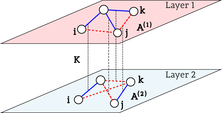
For a bilayer ER network, an assumption is made that nodes are identical in each layer and coupling exists only between link states of the same node pairs in different layers (see Fig. 1).
Considering the topology of a random network, the link connecting a node pair in the first layer might be absent in the second layer. Then, the interlayer interaction between the node pairs would not exist.
The tension arising from discrepancies between relations in different layers for the same pair of agents can also be represented as energy.
Specifically, if the relations are the same, the energy is reduced by a positive amount , whereas if the relations are different, the energy increases by .
The Hamiltonian for a bilayer network, with links and interaction strengths in layers , is
| (2) | ||||
Ground states of the Hamiltonian 2 correspond to cases when all existing triads are balanced in both layers, i.e. and link polarizations are the same in both layers . Note that there are no internal node attributes, and the entire system dynamics considers only changes in link signs . The state of the system will change according to the Hamiltonian in the presence of temperature , which introduces random noise to the dynamics. The temperature represents the unpredictability of human behavior or tolerance towards imbalanced relations in the social systems modeled. The model has a special ground state where all existing links are positive, which is called the paradise state. Other ground states also exist [5, 6, 10], with internally positively connected groups and hostile relations between groups, but we do not investigate them in this paper. Due to thermal fluctuations, at any temperature , the system settles into an equilibrium different than the ground state.
III Analytical approach
III.1 Mean-field approximation for single ER network
Let us start with a monolayer ER graph of size and with the connection probability , where the Hamiltonian is described by Eq.(1). The problem of mean-field description of the Hamiltonian-driven structural balance for a complete graph has been solved before [10]. Our situation differs since a fraction of of the links between agents does not exist. Since the ER network is uncorrelated and features fewer links and triads than the complete graph for , one can expect that the model will behave similarly but with a lower effective interaction strength and, in effect, a lower critical temperature. Let us assume that the nodes and are connected by a link. The polarization of this link is a stochastically fluctuating variable. Since we consider the system in a constant temperature , the probability of finding the system in a microstate is described by Boltzmann distribution.
| (3) |
where,
| (4) |
is the Hamiltonian part dependent on the state of the link . The expected value can be expressed as
| (5) |
Following the mean-field approach developed in [10], the link interacts with the mean-field that is proportional to rather than with the product of specific link polarizations and . The value of this mean field reflects the mean state of links across the entire system, including the link itself, as we consider them all statistically the same, meaning . Since we want to consider the polarization of existing links, this average will include only links with states . Nonexistent links that we formally considered to have are not included in the average , so the mean link value for the entire network can be written as
| (6) |
where the denominator is an expression equal to the number of links , meaning all existing links. We refer to this mean link sign value as the polarization of the network. Since the sum in Hamiltonian is over all node pairs and , and the mean-field does not include nonexistent links, we must account for that. Each link and exists with a probability , which means that for the product to be non-zero, both links must exist, which happens with a probability since the existence of links is uncorrelated in ER graph. Consequently, we average over products with zero value and products with non-zero value and can therefore express the energy of a given state as:
| (7) |
This is the same equation as the mean-field value for a complete graph derived in [10] except multiplied by a constant factor , allowing us to follow the same reasoning further. From Eq. (3), (5) and (7), a self-consistent equation for the mean link polarization as the function of the temperature can be obtained,
| (8) |
where , and is the number of triads containing a given link in a complete graph. This equation, along with an equation for the tangency of the right-hand side of (8) to the diagonal
| (9) |
form a pair of algebraic equations for and when the discontinuous transition from an ordered to a disordered state occurs [10].
Unfortunately, they have no closed-form analytical solution due to their transcendental nature, but we can see that the only difference from the case of a complete graph studied in [10] is the re-scaling of interaction strength by .
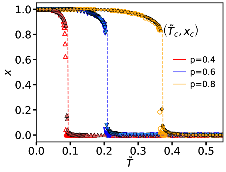
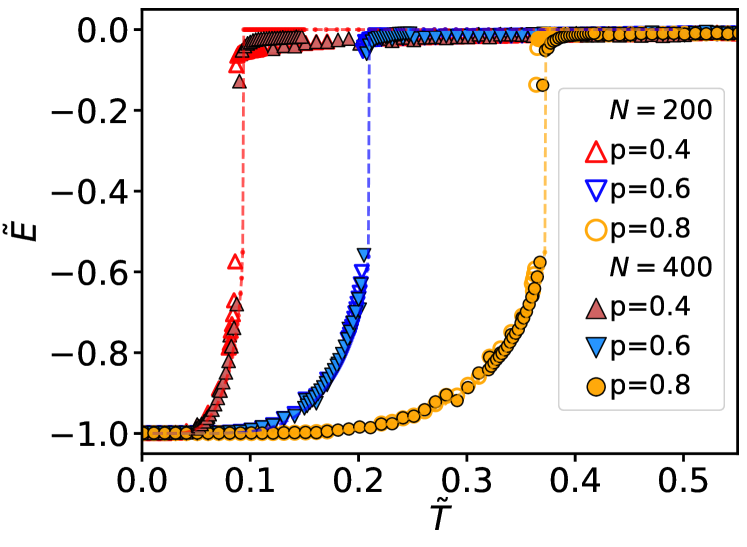
Figure 4a shows the numerical solution of mean polarization for the single layer ER network obtained from the mean-field solution (Eqs. 8, 9) for different values of connection probability . We will assume that the initial condition of the system is a paradise state. In such case, one can anticipate that as the temperature increases, the mean link polarization in equilibrium decreases from a fully polarized state () and reaches where a discontinuous transition occurs at , beyond which the mean polarization becomes zero. The numerical solution [10] yields , independent of model parameters. The critical temperature can be expressed as
| (10) |
where is also independent of model parameters. From the above equation, a normalized critical temperature can be written as
| (11) |
III.2 Mean-field approximation for bilayer ER network
The extension of mean-field approach to a bilayer network composed of two complete graph layers is discussed in [32], where a pair of coupled links is considered as the elementary subsystem interacting with the mean-field, instead of a single link . Applying the same methodology for a bilayer random graph is not trivial because not all node pairs have links in both layers. If we consider two independent random graphs with a probability of each potential link existing and treat them as two layers of the same duplex graph, then we have node pairs that have links in both layers, node pairs featuring a link only in one of the layers, and node pairs without any links (see Fig. 2).

Since we want to use the mean-field approximation, we can forget about specific positions of links in the structure and pair up all single links in layers and into effectively non-interacting link pairs.
We end up with link pairs coupled with constant and non-interacting link pairs where effective .
This means there is a fraction of all link pairs that have interlayer interactions and fraction that do not.
This approximation works only if both layers share the same density of links and, therefore, have the same mean number of links.
Now, we can follow the same methodology as for the bilayer complete graph [32], except with only a fraction of link pairs featuring interlayer interactions, which means that the mean interaction strength between layers in instead of .
Assuming symmetry between layers and mean link pair polarization across the system
| (12) |
we can then approximate the energy tied to the state as
| (13) |
where .
We can see that in the mean-field approach for bilayer ER graphs, the energy tied to a pair of links is the same as for bilayer complete graph [32], except for two differences: the intralayer interaction strength is scaled by , just as in the case of a single-layered network, and the interlayer interaction strength scaled by due to only fraction of link pairs interacting.
Since this is just a re-scaling of both effective interaction strengths, the behavior of the system should be the same as in the case of the complete graph, except with a modified critical temperature.
Following results of [32] the critical temperature is therefore
| (14) |
where and is a solution of a transcendental equation
| (15) |
that has the same form as the complete graph, except , which depends on .
The normalized critical temperature thus depends on the value of .
Initially, the relationship between and may appear quadratic, suggesting that the critical temperature rises with the square of .
However, considering the dependency of on , the relationship is more complex.
For (corresponding to ), the becomes equivalent to non-interacting layers and features simple quadratic dependence on .
To conclude the results for the mean-field description, if the intralayer interaction strength is scaled to and the interlayer interaction strength is scaled from to , then the system statistical properties are independent of , including the normalized critical temperature and are the same as the case of a complete graph (). This is shown in the inset of Fig. 8.
IV Numerical simulation
Numerical Monte Carlo simulations of the model for a single layer and bilayer ER network have been carried out to verify the analytical calculations presented in the previous section.
We employ an asynchronous Metropolis algorithm, where elementary updates are considered as a time step.
For a single-layered ER network, in each update, a random pair of connected agents is chosen, the difference of energy between configuration with inverted and current configuration is calculated, and the sign of the link is inverted with probability .
For the bilayer network, in each update, two pairs of connected agents and are chosen randomly, each from a different layer.
The energy difference is calculated between a configuration with both link signs inverted and the current configuration, including both intralayer Heider interactions and interlayer coupling.
Finally, both link signs and are inverted with probability .
The simulations were conducted across realizations of ER graph, ranging from a sparser network (with ) to a complete graph , while systematically varying the temperature from in increments of .
This iterative process aims to determine the normalized critical temperature at which the mean link polarization and normalized intralayer energy become zero.
The exact value of is identified as the maximum of the slope obtained from the energy data averaged over realizations, wherein the system’s energy changes from a ground state to a disordered state with higher energy (see Appendix A).
The standard error is also calculated from all the realizations.
To obtain the simulation results, the normalized intralayer and interlayer energies are calculated from the Hamiltonian (2).
The intralayer energy for each layer is normalized to represent the average energy per existing triad, given by
| (16) |
where is the interaction strength for layer and is the number of existing triads in layer (mean value ). We fix the value of intralayer interaction strength , and the interlayer energy is scaled to the average energy value per interacting link pair given by,
| (17) |
where is the interlayer interaction strength and is the number of existing coupled link pairs (mean value .
IV.1 Critical behavior of a single layer ER network
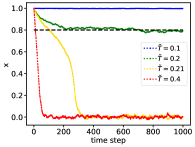
For the paradise state initial condition, the system switches to a disordered state as the temperature surpasses the normalized critical temperature .
Figure 3 illustrates the temporal evolution of across different values of normalized temperature for a system size of . The dashed black line represents the critical value given in sec.III.1.
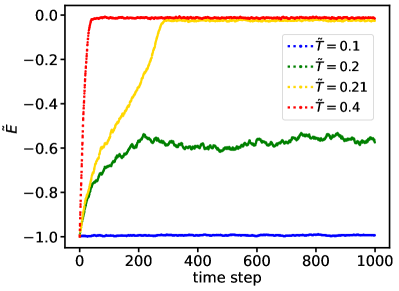
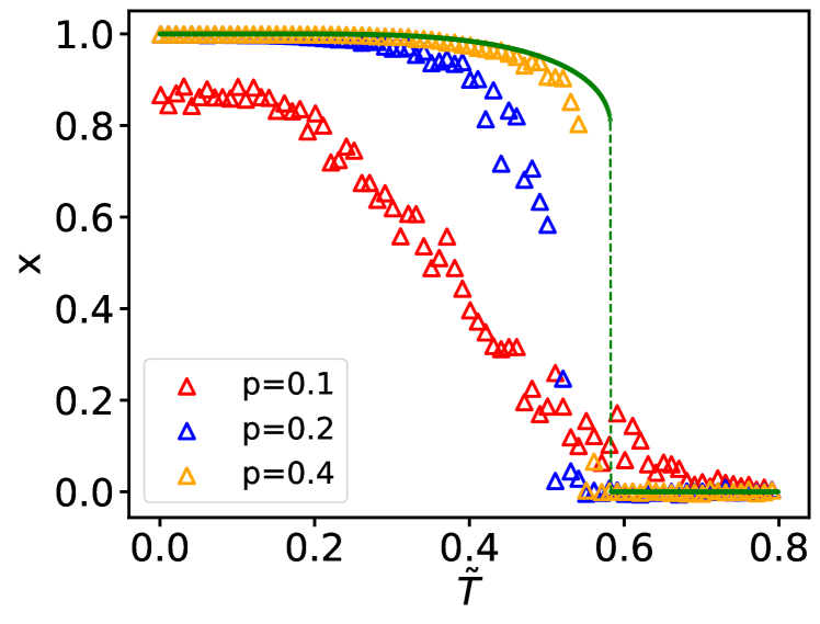
Figure 4 shows the mean link polarization and the corresponding normalized intralayer energy obtained from Eq.16, for different connection probability for network sizes and .
The results indicate that the normalized critical temperature increases as increases.
The intralayer energy approaches zero, and mean polarization fluctuates around zero above the critical temperature.
The critical temperature obtained from the simulations agrees with the mean-field approximation.
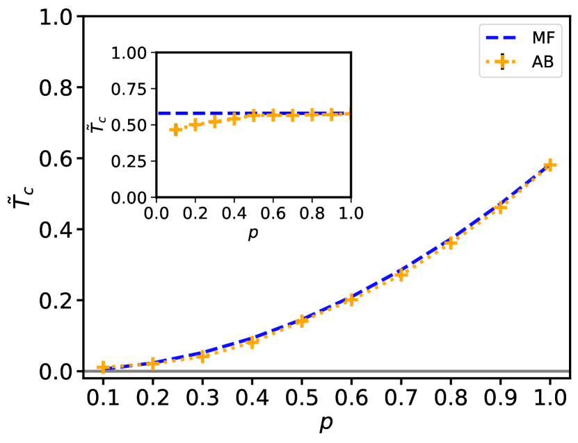
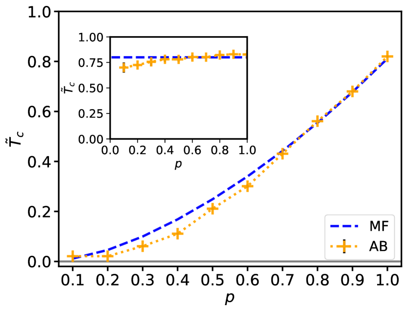
A comparison between the normalized critical temperature predicted by analytical mean-field theory from Eq.14 and those obtained from Monte Carlo simulations is shown in Fig. 5.
The system’s initial condition is the paradise state, and the transition to a disordered state occurs at the normalized critical temperature , above which the ordered state is unstable.
This observed temperature scales with an exponent , determined by fitting a power function to the simulation results.
This scaling aligns well with the expected mean-field prediction, which suggests that the critical temperature should scale with .
The details of the method used to find critical temperature from the simulation data are discussed in Appendix A.
Despite the slight discrepancy observed in the transition point when comparing numerical simulations for with the mean-field approximation, the analytical method is successful.
The fact that the mean-field approximation becomes less accurate as the network becomes sparser is expected since, by its nature, the mean-field captures the complete graph most accurately.
In fact, the case of is special since the sharp first-order transition could not be found in the data, suggesting the disappearance of the expected discontinuous transition, similar to observations of Malarz et al. [31], which means that the agreement between numerical results and analytical predictions should be treated with caution.
The details on this issue are found in Appendix B.
If the connection probability is changed and the interaction strength is simultaneously re-normalized to , the normalized critical temperature remains constant.
This is shown in the Fig.5 inset, where additional simulations were performed with interaction strength , keeping the observed normalized critical temperature roughly constant, equal to the critical temperature for the complete graph with interaction strength .
Similar to the main graph data, the analytical predictions become less accurate as decreases.
IV.2 Distribution of triads
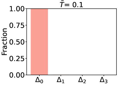
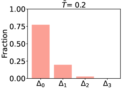
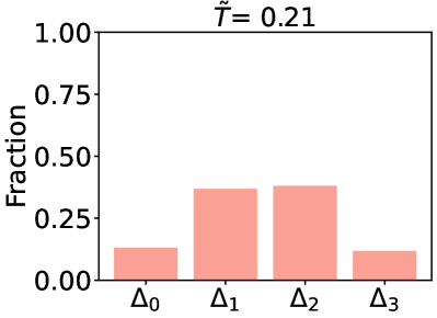
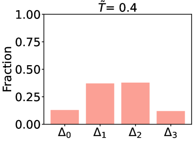
To ensure that our interpretation of the system state based on polarization and energy is correct, we investigated the occurrence frequency of different types of triads within the single-layer ER network. We differentiate triad types by the number of negative links they contain and represent them as , where the subscript indicates the number of negative links. The balance of a triad is characterized by the product of the signs of its edges, so a triad of type and (even number of negative links) are balanced, and the triads of type and (odd number of negative links) are unbalanced. When the ER graph is initiated with paradise state , our findings reveal that at low temperatures (as illustrated in Fig. 6), practically all triads are in a balanced configuration, indicating the paradise state. As long as the temperature remains below the normalized critical temperature , the network maintains a majority of triads of type , with fluctuations resulting in a significant fraction of . Once the temperature exceeds , the distribution of triads undergoes a dramatic transformation. Above the critical temperature, the distribution of triads is dominated by entropy, with triads and being approximately three times more prevalent than and , as expected from a random distribution of link signs in a network. A small influence of Heider balance can still be observed, with balanced triads and being slightly more popular than their imbalanced counterparts and .
IV.3 Effect of coupling for a bilayer ER network
In the case of a bilayer ER network, if both layers are in the paradise state, then the system is balanced.
This scenario reflects a condition where all intralayer relationships are positive , leading to a harmonious and fully cooperative network environment across both layers.
In our simulations, the interaction parameters in both layers of the network are kept as , reflecting uniformity in the strength of interactions across the network layers.
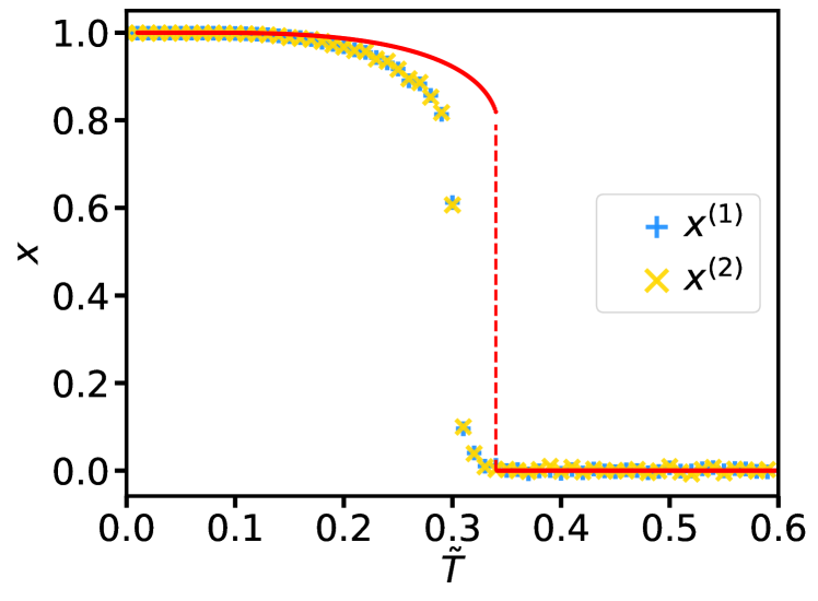
Up to temperature , the system remains polarized with , while above , the system discontinuously changes to a disordered state .
This is shown in Figure 7, where a consistent alignment is observed across both layers of the system below normalized critical temperature , and above , the mean polarization drops to around zero, reflecting a disordered state.
The critical temperature derived from these results is lower than that predicted by the mean-field approximation.
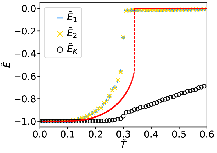
At the same time as a change in polarization occurs, a discontinuous behavior is observed for the normalized intralayer energies and , that converge towards zero.
A small local ordering persists, lowering the mean value of energy below zero.
The normalized interlayer energy also changes but displays negative values both above and below the critical temperature.
This observation suggests a significant, partial alignment of link signs across different layers, even amidst the disordered state above .
This behavior is similar to the case of a complete graph (see ref.[32])
Figure 8 compares the normalized critical temperature predicted by the mean-field theory and temperature values obtained from Monte Carlo simulations where both layers started from a paradise state.
The critical temperature increases with and is in good agreement with the analytical results for high .
The discrepancy for low appears due to the sparser network behavior not being described well by the mean-field approximation.
Suppose the connection probability of the network is changed, and the intralayer interaction strength is simultaneously re-scaled to and the interlayer strength re-normalized to . In such a case, the critical temperature estimated from analytical mean-field calculations (Eq. 14) is independent of the parameter , and this prediction is confirmed by numerical simulations presented in the inset of Fig.8.
V Conclusions
We have investigated the behavior of the Heider balance model in Erdös-Rényi random graphs, in particular its transition from the ordered paradise state to disorder, both in a single-layer and a bilayer network.
We find that the critical temperature of this transition in a single network scales with network density as , while for a bilayer network, the scaling becomes much more complex.
In fact, the model with Heider interaction strength and interlayer interaction strength behaves the same as in complete graphs with Heider interaction strength and interlayer interaction strength , provided that is not too small. This scaling with network density is unlike typical two-body interaction models like the Ising model, where critical temperature simply scales with linearly [24, 23].
The difference in re-scaling of intralayer and interlayer interaction strength comes from the fact that the number of triads a given link is involved in scales faster with link density than the probability that a link in one layer will have a matching link in the other layer.
This behavior has been described analytically using a mean-field approach and verified using numerical Monte Carlo simulations, although the prediction is inaccurate for networks with low link density.
The behavior of the Heider structural balance in random graphs has already been investigated before [30, 31].
While [30] studied the problem, their analytical description focused on critical temperature for transition to disorder in the case of initially disordered networks, which corresponds to the temperature above which disorder becomes a stable state.
Due to system multistability, also described in [30], this is not the same as the temperature where order becomes unstable, which we have focused on in our work.
Similarly, [31] only investigates the temperature where initial disorder can prevail, not when order disappears, but notes that such a transition becomes continuous if the density of the network is low enough.
This is similar to the situation observed in our numerical results for , where the transition from paradise to disorder seems to lose its discontinuous character.
The normalized critical temperature we investigated is expected to scale as , and a fit to numerical results suggests an even slightly higher exponent. In contrast, the critical temperature found in [31] (which we will refer to as to conform with previous literature [10, 32]) shows slower scaling with the exponent .
Overall, we have demonstrated that although ER network structure contains a topological disorder, the spontaneous order in structural balance for ER graphs can still exist below a critical temperature, and system critical properties can be analytically described by a properly adapted mean-field approach, similar to the one used for complete graphs.
Acknowledgements.
This research received funding from the Polish National Science Center under Alphorn Grant No. 2019/01/Y/ST2/00058. This work was funded by the European Union under the Horizon Europe grant OMINO (Grant No. 101086321) and was also co-financed with funds from the Polish Ministry of Education and Science under the program entitled International Co-Financed Projects.Appendix A Finding critical temperature from numerical simulations
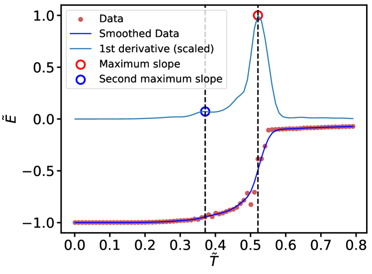
The critical temperature calculated from the simulation is determined by identifying the maximum of the slope where the system’s normalized energy, as described by Eq. (16), changes from the ground state to a disordered state with higher energy.
The normalized energy is used to identify the critical temperature instead of mean polarization because the energy is less susceptible to fluctuations and early state transition due to finite size effects (partially seen in Fig. 4), especially for low values of .
This difference in behavior makes energy a more reliable observable for determining the critical temperature.
To determine the critical temperature, we apply Gaussian kernel smoothing to the normalized energy data, averaging over realizations.
A key component in Gaussian smoothing is selecting the appropriate value, which defines the width of the Gaussian distribution used to smooth the data.
The correct choice of significantly impacts the clarity and accuracy of the results, especially for low values of where the transition behavior is rather noisy.
To select the optimal value of , we evaluate a range of possible values starting from .
For each value of , we identify the two largest maxima of the slope.
If there is only one maximum or the ratio between the largest and second-largest maxima is or more (arbitrary factor), we conclude that the smoothing is optimal, and we have found the one true maximum and take it as our observed critical temperature.
If this condition is not fulfilled, we increase by and try again until we have smoothed the data enough for the above criteria to be fulfilled.
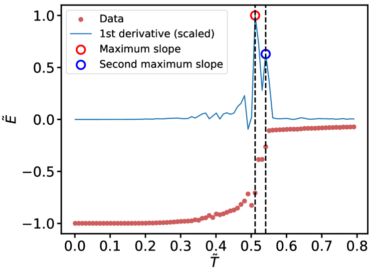
Figure 9 illustrates finding slope maxima for unsmoothed and smoothed data.
Since the original data is discrete, the smoothed data retains this discrete nature.
To find slope maxima, we calculate the numerical derivatives of the smoothed data.
Gradients are computed using central differences for internal points and first differences at the boundaries.
Appendix B Continuity of transition for sparse graphs
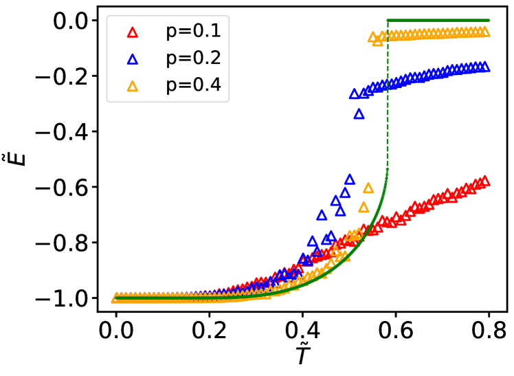
In the data obtained from simulations for low , the discontinuity of the transition from ordered to disordered state is not evident. Due to the close proximity of critical temperatures to zero, this is not very clear for the data underlying the main graph in Fig. 5, but it can be seen much clearer for the re-scaled inset data. Figure 10 shows the behavior of the polarization and normalized energy for sparse ER networks when For , the transition between ordered and disordered states does not appear to be discontinuous, even if we allow for finite-size effects always present in the simulations. This means that while we are able to calculate critical temperature for using data shown in Fig. 10b, and their values are relatively close to those expected from the analytical approach, the nature of the transition is not the same and the numerical results should be considered with caution. Note that although the effect is similar to that observed by Malarz et al. [31] for a disorder to order transition, the transition investigated is different, which means neither our results can be considered a confirmation of that of Malarz et al. nor vice versa.
References
- Heider [1946] F. Heider, J. Psychol. 21, 107 – 112 (1946).
- Cartwright and Harary [1956] D. Cartwright and F. Harary, Psychol. Rev. 63, 277 – 293 (1956).
- Marvel et al. [2009] S. A. Marvel, S. H. Strogatz, and J. M. Kleinberg, Phys. Rev. Lett. 103, 198701 (2009).
- Marvel et al. [2011] S. A. Marvel, J. Kleinberg, R. D. Kleinberg, and S. H. Strogatz, Proc. Nat. Acad. Sci. U.S.A. 108, 1771 (2011).
- Antal et al. [2005] T. Antal, P. L. Krapivsky, and S. Redner, Phys. Rev. E 72, 036121 (2005).
- Antal et al. [2006] T. Antal, P. Krapivsky, and S. Redner, Physica D 224, 130 – 136 (2006).
- Abell and Ludwig [2009] P. Abell and M. Ludwig, Journal of Mathematical Sociology 33, 129 (2009).
- Belaza et al. [2017] A. M. Belaza, K. Hoefman, J. Ryckebusch, A. Bramson, M. van den Heuvel, and K. Schoors, PLOS ONE 12, 1 (2017).
- Rabbani et al. [2019] F. Rabbani, A. H. Shirazi, and G. R. Jafari, Phys. Rev. E 99, 062302 (2019).
- Malarz and Hołyst [2022] K. Malarz and J. A. Hołyst, Phys. Rev. E 106, 064139 (2022).
- Summers and Shames [2013] T. H. Summers and I. Shames, EPL 103, 18001 (2013).
- Facchetti et al. [2011] G. Facchetti, G. Iacono, and C. Altafini, Proc. Nat. Acad. Sci. U.S.A. 108, 20953 – 20958 (2011).
- Doreian and Mrvar [2015] P. Doreian and A. Mrvar, J. Social Structure 16, 1 – 49 (2015).
- Yang et al. [2022] M. Yang, X. Wang, L. Ma, Q. He, and M. Huang, Neural Comput. Appl. 34, 16683–16700 (2022).
- Burghardt and Maoz [2020] K. Burghardt and Z. Maoz, Journal of Complex Networks 8, cnaa001 (2020).
- Pham et al. [2022] T. M. Pham, J. Korbel, R. Hanel, and S. Thurner, Proceedings of the National Academy of Sciences 119, e2121103119 (2022).
- Górski et al. [2020] P. J. Górski, K. Bochenina, J. A. Hołyst, and R. M. D’Souza, Physical Review Letters 125, 078302 (2020).
- Erdös and Rényi [1959] P. Erdös and A. Rényi, Publicationes Mathematicae Debrecen 6, 290 (1959).
- Winkler and Reichardt [2013] M. Winkler and J. Reichardt, Physical Review E 88, 022805 (2013).
- Itzkovitz and Alon [2005] S. Itzkovitz and U. Alon, Physical Review E 71, 026117 (2005).
- Shi and Shi [2014] H. Shi and L. Shi, Plos One 9, e99634 (2014).
- Callaway et al. [2000] D. S. Callaway, M. E. J. Newman, S. H. Strogatz, and D. J. Watts, Phys. Rev. Lett. 85, 5468 (2000).
- Dorogovtsev et al. [2002] S. Dorogovtsev, A. Goltsev, and J. Mendes, Phys. Rev. E 66, 10.1103/PhysRevE.66.016104 (2002).
- Dembo and Montanari [2010] A. Dembo and A. Montanari, The Annals of Applied Probability 20, 565 (2010).
- Vilone and Castellano [2004] D. Vilone and C. Castellano, Phys. Rev. E 69, 016109 (2004).
- Pereira and Moreira [2005] L. F. Pereira and F. B. Moreira, Physical Review E 71, 016123 (2005).
- Pournaki et al. [2023] A. Pournaki, E. Olbrich, S. Banisch, and K. Klemm, Physical Review E 107, 054112 (2023).
- Frachebourg and Krapivsky [1996] L. Frachebourg and P. L. Krapivsky, Phys. Rev. E 53, R3009 (1996).
- Sood and Redner [2005] V. Sood and S. Redner, Phys. Rev. Lett. 94, 178701 (2005).
- Masoumi et al. [2022] R. Masoumi, F. Oloomi, S. Sajjadi, A. Shirazi, and G. Jafari, Physical Review E 106, 034309 (2022).
- Malarz and Wołoszyn [2023] K. Malarz and M. Wołoszyn, Chaos 33, 10.1063/5.0141019 (2023).
- Mohandas et al. [2024] K. Mohandas, K. Suchecki, and J. A. Hołyst, Physical Review E 109, 044306 (2024).
- Górski et al. [2017] P. J. Górski, K. Kułakowski, P. Gawroński, and J. A. Hołyst, Sci. Rep. 7, 16047 (2017).