Preasymptotic error estimates of EEM and CIP-EEM for the time-harmonic Maxwell equations with large wave number

Abstract.

Preasymptotic error estimates are derived for the linear edge element method (EEM) and the linear ${\bm{H}}(\operatorname{\bm{\mathrm{curl}}})$-conforming interior penalty edge element method (CIP-EEM) for the time-harmonic Maxwell equations with large wave number. It is shown that under the mesh condition that $\kappa^{3}h^{2}$ is sufficiently small, the errors of the solutions to both methods are bounded by $\mathcal{O}(\kappa h+\kappa^{3}h^{2})$ in the energy norm and $\mathcal{O}(\kappa h^{2}+\kappa^{2}h^{2})$ in the ${\bm{L}}^{2}$ norm, where $\kappa$ is the wave number and $h$ is the mesh size. Numerical tests are provided to verify our theoretical results and to illustrate the potential of CIP-EEM in significantly reducing the pollution effect.

1. Introduction

In this paper, we consider the following time-harmonic Maxwell equations for the electric field $\bm{E}$ with the standard impedance boundary condition:

$$\operatorname{\bm{\mathrm{curl}}}\operatorname{\bm{\mathrm{curl}}}\bm{E}-\kappa^{2}\bm{E} =\bm{f}\qquad {\rm in}\ \Omega,$$ (1.1)

$$\operatorname{\bm{\mathrm{curl}}}\bm{E}\times\bm{\nu}-\bm{\mathrm{i}}\kappa\lambda\bm{E}_{T} =\bm{g}\qquad {\rm on}\ \Gamma:=\partial\Omega,$$ (1.2)

where $\Omega\subset\mathbb{R}^{3}$ is a bounded domain with a $C^{2}$ boundary. Here, $\bm{\mathrm{i}}=\sqrt{-1}$ denotes the imaginary unit while $\bm{\nu}$ denotes the unit outward normal to $\Gamma$ and $\bm{E}_{T}:=(\bm{\nu}\times\bm{E})\times\bm{\nu}$ is the tangential component of $\bm{E}$ on $\Gamma$. Additionally, $\kappa>0$ is the wave number, and $\lambda>0$ is known as the impedance constant. The right-hand side $\bm{f}$ is related to a given current density (cf. [31]). It is assumed that $\operatorname{\bm{\mathrm{div}}}\bm{f}=0$ in $\Omega$ and $\bm{g}_{T}=\bm{g}$ on $\Gamma$ (i.e. $\bm{g}\cdot\bm{\nu}=0$). The time-harmonic Maxwell equations govern the propagation of electromagnetic waves at a specified frequency, serving as fundamental tools for comprehending and forecasting electromagnetic field behaviors across diverse applications such as telecommunications, radar, optics, and electromagnetic sensing. Accurate numerical approximation of these equations is imperative for predicting wave propagation phenomena in practical scenarios.

Since the seminal contributions of Nédélec [34, 35], the edge element method (EEM) has garnered significant popularity and become a central tool for addressing electromagnetic field problems. Subsequently, a substantial body of literature has emerged studying EEM for solving the Maxwell equations, we refer the readers to [31, 18, 23] and the references therein. For time-harmonic Maxwell problems with impedance boundary conditions, Monk [31, Chapter 7] and Gatica and Meddahi [17] have investigated the convergence and error estimation of EEM under the condition that the mesh size is sufficiently small. Both of these results are $\kappa$-implicit, meaning they do not discuss the influence of $\kappa$ on the error, and thus are applicable primarily to problems with small wave numbers.

However, in scenarios involving large wave numbers, a large number of studies of the finite element methods (FEMs) for Helmholtz equations [5, 22, 27, 28, 39, 13, 44, 43] indicate that the EEM of fixed order may also suffer from the well-known “pollution effect”, i.e., compared to the best approximation from the discrete space, the approximation ability of the solution to the EEM (with fixed order) gets worse and worse as the wave number $\kappa$ increases. Clearly, estimating the pollution error is significant both in theory and practice, and it has always been interesting to develop numerical methods with less pollution error. Unfortunately, rigorous pollution-error analyses for the EEM for the time-harmonic Maxwell equations are still unavailable in the literature. We recall that the term “asymptotic error estimate” refers to the error estimate without pollution error and the term “preasymptotic error estimate” refers to the estimate with non-negligible pollution effect.

The latest asymptotic error analysis for the time-harmonic Maxwell equations was conducted by Melenk and Sauter in [29, 30], where the first type Nédélec $hp$-EEM for solving the time-harmonic Maxwell equations with transparent boundary condition and impedance boundary condition has been studied. Using the so-called “regularity decomposition” technique, they show that the $hp$-EEM is pollution-free under the following scale resolution conditions:

$$\frac{\kappa h}{p}\leq c_{1}\qquad\mbox{ and }\qquad p\geq c_{2}\ln\kappa,$$ (1.3)

where $h$ is the mesh size, $c_{2}$ is an arbitrary positive number and $c_{1}>0$ is sufficiently small. The resolution condition $\kappa h/p\leq c_{1}$ is natural for resolving the oscillatory behavior of the solution, and the side constraint $p\geq c_{2}\ln\kappa$ suppresses the pollution effect. The above result highlights the advantages of high-order EEM, representing a breakthrough in the analysis of the time-harmonic Maxwell equations in the large wave number regime. But for fixed order, say second order EEM of the first type, the above two works require that $k^{8}h$ is sufficiently small (see [29, Remark 4.19]) for the case of transparent boundary condition and $k^{2}h$ is sufficiently small for the case of impedance boundary condition, respectively, which are too strict in $h$. For the special case $\bm{g}=\bm{0}$ in problem (1.1)–(1.2), Nicaise and Tomezyk [37, 36], using $h$- and $hp$-FEM with Lagrange elements, performed asymptotic error analyses for a regularized Maxwell system(cf. [11, § 4.5d]).

Recently, Lu  et al.[26] proposed an ${\bm{H}}(\operatorname{\bm{\mathrm{curl}}})$-conforming interior penalty edge element method (CIP-EEM), which uses the same approximation space as EEM but modifies the sesquilinear form by adding a least squares term penalizing the jump of the tangential components of the $\operatorname{\bm{\mathrm{curl}}}$ of the discrete solution at mesh interfaces. Using the so-called “stability-error iterative improvement” technique [15], they proved that the CIP-EEM with pure imaginary penalty parameter $\gamma=-\bm{\mathrm{i}}\gamma_{\bm{\mathrm{i}}}$ is absolute stable (that is, stable for any $\kappa$ and $h$) and obtained the following error estimate under the conditions $\gamma_{\bm{\mathrm{i}}}\simeq 1$ and $\kappa^{3}h^{2}=\mathcal{O}(1)$:

$$\interleave\bm{E}-{\bm{E}}_{h}\interleave=\mathcal{O}(\kappa h+\kappa^{3}h^{2}),$$ (1.4)

where $\interleave\cdot\interleave=\big{(}\left\|\operatorname{\bm{\mathrm{curl}}}\cdot\right\|^{2}+\kappa^{2}\|\cdot\|^{2}+\kappa\lambda\|\cdot_{T}\|^{2}_{\Gamma}\big{)}^{\frac{1}{2}}$ is the energy norm. This is a closely related result. However, this result does not encompass the classical EEM since $\gamma$ cannot be zero there. For wave-number-explicit error analyses of various discontinuous Galerkin (DG) methods, we refer to [16, 14, 20].

The purpose of this paper is twofold. First, we focus on the preasymptotic error analysis of the EEM and provide the first such results in the literature for the EEM using the linear Nédélec element of the second type. To be precise, we have proved the following error estimate for the solution ${\bm{E}}_{h}$ to the linear EEM, under the mesh condition that $\kappa^{3}h^{2}$ is sufficiently small:

$$\interleave\bm{E}-{\bm{E}}_{h}\interleave=\mathcal{O}(\kappa h+\kappa^{3}h^{2}).$$ (1.5)

Clearly, the first term $\mathcal{O}(\kappa h)$ on the right-hand side of (1.5) is of the same order as the error of the best approximation, which can be reduced by putting enough points per wavelength. However, the second term $\mathcal{O}(\kappa^{3}h^{2})$ will get out of control as the wave number $\kappa$ increases, no matter how many points are put per wavelength, as long as the number of them is fixed. Therefore, the second term is the pollution error which dominates the error bound when $\kappa^{2}h$ is large. Moreover, the following ${\bm{L}}^{2}$ error estimate has also been proved under the same mesh condition:

$$\kappa\|\bm{E}-{\bm{E}}_{h}\|=\mathcal{O}\big{(}(\kappa h)^{2}+\kappa^{3}h^{2}\big{)}.$$ (1.6)

We would like to mention that, in order to prove the error estimates (1.5)–(1.6), thanks to the recent work [9], we derive a wave-number-explicit ${\bm{H}}^{2}$ regularity estimate (see (3.3)) for the continuous problem on the domain with only $C^{2}$-smooth boundary. A similar estimate was proved in [25] for a domain with $C^{3}$ boundary. Secondly, we extend the result in [26] for the CIP-EEM to a more general case, i.e., the linear CIP-EEM with complex penalty parameters $\gamma=\gamma_{r}-\bm{\mathrm{i}}\gamma_{i}$. To be precise, we prove that (1.4) still holds, if $\operatorname{{Re}}\gamma\geq-\alpha_{0}$, $\operatorname{{Im}}\gamma\leq 0$, $|\gamma|\leq C$, and $\kappa^{3}h^{2}\leq C_{0}$, for some positive constants $C_{0}$ and $\alpha_{0}$ independent of $\kappa$ and $h$. Such an extension is meaningful since the penalty parameters that can greatly reduce the pollution error are usually close to negative real numbers (see Section 6), which is not covered by the theory given in [26]. By the way, the divergence-free constraint on the source term $\bm{f}$ in [26] is dropped in this paper. Compared with the linear EEM, the linear CIP-EEM provides a candidate with enhanced stability and low pollution effects. We would like to mention that due to their easy of implementation, low-order methods are still attractive in many applications, especially for those low-regularity problems where a higher-order method cannot achieve its full convergence rate.

The key idea in our preasymptotic analysis for the EEM and CIP-EEM is to first prove stability estimates for the discrete solution ${\bm{E}}_{h}$, in which a delicate decomposition of ${\bm{E}}_{h}$ (see (4.1)) and a so-called “modified duality argument” technique play important roles, and then use the obtained stability estimates to derive the desired error estimates. The “modified duality argument” technique was first used to derive preasymptotic error estimates for the FEM for Helmholtz equations with large wave numbers [44, 13]. Here we extend it to derive stability estimates for the EEM. We would like to mention that our proofs are highly non-trivial. The “stability-error iterative improvement” technique used in [26] does not work for the EEM or CIP-EEM with general parameters. We had also tried to derive preasymptotic error estimates for the EEM by mimicking the usual process (see, e.g., [31]), including using the modified duality argument to derive the error estimates directly, but failed. The preasymptotic error analysis of higher-order EEM and CIP-EEM necessitates additional technical tools and will be investigated in another work.

The remainder of this paper is organized as follows. In Section 2, we formulate the EEM and the CIP-EEM. Section 3 introduces some preliminary results about the stability estimates and some error estimates of some ${\bm{H}}(\operatorname{\bm{\mathrm{curl}}})$-elliptic projections. In Section 4, we first establish discrete stability estimates for the EEM solution. Then we prove the preasymptotic error estimates of the EEM for the time-harmonic Maxwell problem. In Section 5, we extend the results of preasymptotic error estimates to the linear CIP-EEM with general penalty parameters. Finally, in Section 6, we present some numerical examples to verify our theoretical findings and the great potential of the CIP-EEM to reduce the pollution errors.

Throughout this paper, we use notations $A\lesssim B$ and $A\gtrsim B$ for the inequalities $A\leq CB$ and $A\geq CB$, where $C$ is a positive number independent of the mesh size $h$ and the wave number $\kappa$, but the value of which can vary in different occurrences. $A\simeq B$ is a shorthand notation for the statement $A\leq CB$ and $B\leq CA$. We also denote by $C_{\kappa h}$ a generic constant which may depends on $\kappa h$ but satisfies $C_{\kappa h}\lesssim 1$ when $\kappa h\lesssim 1$.

For simplicity, we suppose $\lambda\simeq 1$, $\kappa{\gtrsim 1}$. We also assume that the domain $\Omega$ is strictly star-shaped with respect to a point ${\bm{x}}_{0}\in\Omega$, that is, $({\bm{x}}-{\bm{x}}_{0})\cdot\bm{\nu}\gtrsim 1\quad\forall\bm{x}\in\Gamma$.

2. Formulations of EEM and CIP-EEM

In order to formulate the two methods, we first introduce some notations. For a domain $D\subset\mathbb{R}^{3}$ with Lipschitz boundary $\partial D$, we shall use the standard Sobolev space $H^{s}(D)$, its norm $\|\cdot\|_{s,D}$, seminorm $|\cdot|_{s,D}$, and inner product. We refer to [1, 6, 31] for their definitions. If the functions are vector-valued we shall indicate these function spaces by boldface symbols, e.g., ${\bm{H}}^{s}(D)$. In particular, $(\cdot,\cdot)_{D}$ and $\langle\cdot,\cdot\rangle_{\Sigma}$ for $\Sigma\subset\partial D$ denote the ${\bm{L}}^{2}$-inner product on complex-valued ${\bm{L}}^{2}(D)$ and ${\bm{L}}^{2}(\Sigma)$ spaces, respectively. For simplicity, we shall use the shorthands:

$$(\cdot,\cdot):=(\cdot,\cdot)_{\Omega},\;\langle\cdot,\cdot\rangle:=\langle\cdot,\cdot\rangle_{\Gamma},\;|{\bm{v}}|_{s}:=|{\bm{v}}|_{s,\Omega},\;\|{\bm{v}}\|_{s}:=\|{\bm{v}}\|_{s,\Omega},\;\|{\bm{v}}\|:=\|{\bm{v}}\|_{0,\Omega},\;\text{and}\;\|{\bm{v}}\|_{\Gamma}:=\|{\bm{v}}\|_{0,\Gamma}.$$

We introduce the space

$${\bm{H}}(\operatorname{\bm{\mathrm{curl}}};\Omega):=\{{\bm{v}}\in{\bm{L}}^{2}{(\Omega)}:\operatorname{\bm{\mathrm{curl}}}{\bm{v}}\in{\bm{L}}^{2}{(\Omega)}\},$$

$${\bm{H}}^{1}(\operatorname{\bm{\mathrm{curl}}};\Omega):=\{{\bm{v}}\in{\bm{H}}^{1}{(\Omega)}:\operatorname{\bm{\mathrm{curl}}}{\bm{v}}\in{\bm{H}}^{1}{(\Omega)}\}\quad\text{with norms}$$

$$\left\|\bm{v}\right\|_{{\bm{H}}(\operatorname{\bm{\mathrm{curl}}})}:=\big{(}\left\|\operatorname{\bm{\mathrm{curl}}}\bm{v}\right\|^{2}+\left\|\bm{v}\right\|^{2}\big{)}^{\frac{1}{2}},$$

$$\left\|\bm{v}\right\|_{{\bm{H}}^{1}(\operatorname{\bm{\mathrm{curl}}})}:=\big{(}\left\|\operatorname{\bm{\mathrm{curl}}}\bm{v}\right\|_{1}^{2}+\left\|\bm{v}\right\|_{1}^{2}\big{)}^{\frac{1}{2}}\quad\text{and seminorm}$$

$$|\bm{v}|_{{\bm{H}}^{1}(\operatorname{\bm{\mathrm{curl}}})}:=\big{(}|\operatorname{\bm{\mathrm{curl}}}\bm{v}|_{1}^{2}+|\bm{v}|_{1}^{2}\big{)}^{\frac{1}{2}}.$$

Let

$$H_{0}^{1}(\Omega) :=\big{\{}v\in H^{1}(\Omega):v|_{\Gamma}=0\big{\}},$$

$${\bm{H}}_{0}(\operatorname{\bm{\mathrm{curl}}};\Omega) :=\big{\{}{\bm{v}}\in{\bm{H}}(\operatorname{\bm{\mathrm{curl}}};\Omega):{\bm{v}}\times\bm{\nu}|_{\Gamma}=0\big{\}},$$

where $v|_{\Gamma}$ is understood as the trace from $H^{1}(\Omega)$ to $H^{\frac{1}{2}}(\Gamma)$ and ${\bm{v}}\times\bm{\nu}|_{\Gamma}$ is the tangential trace from ${\bm{H}}(\operatorname{\bm{\mathrm{curl}}};\Omega)$ to ${\bm{H}}_{\operatorname{\bm{\mathrm{div}}}}^{-1/2}(\Gamma)$. Similarly, we will understand ${\bm{v}}_{T}$ as the tangential trace from ${\bm{H}}(\operatorname{\bm{\mathrm{curl}}};\Omega)$ to ${\bm{H}}_{\operatorname{\bm{\mathrm{curl}}}}^{-1/2}(\Gamma)$ (see, e.g., [31, 29]).

Next we define the “energy” space

$$\bm{V} :=\big{\{}{\bm{v}}\in{\bm{H}}(\operatorname{\bm{\mathrm{curl}}};\Omega):{{\bm{v}}_{T}\in{\bm{L}}^{2}(\Gamma)\big{\}}}\quad\text{with norm}$$

$${\interleave{\bm{v}}\interleave} :=\big{(}\left\|\operatorname{\bm{\mathrm{curl}}}\bm{v}\right\|^{2}+\kappa^{2}\|{\bm{v}}\|^{2}+\kappa\lambda\|{\bm{v}}_{T}\|^{2}_{\Gamma}\big{)}^{\frac{1}{2}},$$

and introduce the following sesquilinear form on $\bm{V}\times\bm{V}$:

$$a\left({\bm{u}},{\bm{v}}\right):=\left(\operatorname{\bm{\mathrm{curl}}}{\bm{u}},\operatorname{\bm{\mathrm{curl}}}{\bm{v}}\right)-\kappa^{2}\left({\bm{u}},{\bm{v}}\right)-\bm{\mathrm{i}}\kappa\lambda\left\langle{{\bm{u}}_{T},{\bm{v}}_{T}}\right\rangle.$$ (2.1)

Then the variational formulation of (1.1)–(1.2) reads as: Find $\bm{E}\in\bm{V}$ such that

$$a\left(\bm{E},{\bm{v}}\right)=\left(\bm{f},{\bm{v}}\right)+\left\langle\bm{g},{{\bm{v}}_{T}}\right\rangle\quad\forall{\bm{v}}\in{\bm{V}}.$$ (2.2)

To discretize (2.2), we follow [30] to introduce a regular and quasi-uniform triangulation $\mathcal{T}_{h}$ of $\Omega$ which satisfies:

1. The (closed) elements $K\in\mathcal{T}_{h}$ cover $\Omega$, i.e., $\bar{\Omega}=\cup_{K\in\mathcal{T}_{h}}K$.

2. Associated with each element $K$ is the element map, a $C^{1}$-diffeomorphism $F_{K}:\hat{K}\rightarrow K$. The set $\hat{K}$ is the reference tetrahedron. Denoting $h_{K}:=\operatorname{{diam}}(K)$, there holds, with some shape-regularity constant $\sigma$,

   $$h_{K}^{-1}\left\|F_{K}^{\prime}\right\|_{L^{\infty}(\hat{K})}+h_{K}\left\|(F_{K}^{\prime})^{-1}\right\|_{L^{\infty}(\hat{K})}\leq\sigma,$$

   where $F_{K}^{\prime}$ is the Jacobian matrix of $F_{K}$.

3. The intersection of two elements is only empty, a vertex, an edge, a face, or they coincide (here, vertices, edges, and faces are the images of the corresponding entities on the reference element $\hat{K}$). The parameterization of common edges or faces is compatible. That is, if two elements $K$, $K^{\prime}$ share an edge (i.e., $F_{K}(e)=F_{K^{\prime}}(e^{\prime})$ for edges $e,e^{\prime}$ of $\hat{K}$ ) or a face (i.e., $F_{K}({\mathsf{f}})=F_{K^{\prime}}(\mathsf{f}^{\prime})$ for faces $\mathsf{f},\mathsf{f}^{\prime}$ of $\hat{K}$), then $F^{-1}_{K}\circ F_{K^{\prime}}:\mathsf{f}^{\prime}\rightarrow\mathsf{f}$ is an affine isomorphism.

The set of all faces of $\mathcal{T}_{h}$ is denoted by $\mathcal{F}_{h}$ , and the set of all interior faces by $\mathcal{F}_{h}^{I}$. For any $\mathsf{f}\in\mathcal{F}_{h}$, let $h_{\mathsf{f}}:=\operatorname{{diam}}(\mathsf{f})$. Denote by $h:=\max_{K\in\mathcal{T}_{h}}h_{K}$.

Let $\bm{V}_{h}$ be the first order Nédélec edge element space of the second type (see [31, (3.76)]):

$$\bm{V}_{h}:=\Big{\{}{\bm{v}}_{h}\in\bm{V}:\;(F_{K}^{\prime})^{T}(\left.{\bm{v}}_{h}\right|_{K})\circ F_{K}\in\big{(}\mathcal{P}_{1}(\hat{K})\big{)}^{3}\quad\forall K\in\mathcal{T}_{h}\Big{\}},$$ (2.3)

where $\mathcal{P}_{1}(\hat{K})$ denotes the set of linear polynomials on $\hat{K}$. The EEM for the Maxwell problem (1.1)–(1.2) reads as: Find $\bm{E}_{h}\in\bm{V}_{h}$ such that

$$a\left({\bm{E}}_{h},{\bm{v}}_{h}\right)=\left(\bm{f},{\bm{v}}_{h}\right)+\left\langle\bm{g},{\bm{v}}_{h,T}\right\rangle\quad\forall{\bm{v}}_{h}\in\bm{V}_{h}.$$ (2.4)

To formulate the CIP-EEM, we define the jump of the tangential components of $\operatorname{\bm{\mathrm{curl}}}{\bm{u}}$ on an interior face $\mathsf{f}=\partial K^{-}\cap\partial K^{+}$ :

$${\llbracket\operatorname{\bm{\mathrm{curl}}}{\bm{u}}\rrbracket}:=\operatorname{\bm{\mathrm{curl}}}{\bm{u}}|_{K^{-}}\times\bm{\nu}_{K^{-}}+\operatorname{\bm{\mathrm{curl}}}{\bm{u}}|_{K^{+}}\times\bm{\nu}_{K^{+}},$$ (2.5)

where $\bm{\nu}_{K^{-}}$ and $\bm{\nu}_{K^{+}}$ denote the unit outward normal to $\partial K^{-}$ and $\partial K^{+}$, respectively. We introduce the following sesquilinear form consisting of penalty terms on interior faces:

$$\bm{J}({\bm{u}},{\bm{v}}):=\sum_{\mathsf{f}\in\mathcal{F}_{h}^{I}}\gamma_{\mathsf{f}}h_{\mathsf{f}}\langle\llbracket\operatorname{\bm{\mathrm{curl}}}{\bm{u}}\rrbracket,\llbracket\operatorname{\bm{\mathrm{curl}}}{\bm{v}}\rrbracket\rangle_{\mathsf{f}},$$ (2.6)

where $\gamma_{\mathsf{f}}$ are penalty parameters that are allowed to be complex-valued. Then the CIP-EEM is constructed by simply adding $\bm{J}({\bm{E}}_{h},{\bm{v}}_{h})$ to the left-hand side of EEM (2.4), which is to find $\bm{E}_{h}\in\bm{V}_{h}$ such that

$$a_{\gamma}\left({\bm{E}}_{h},{\bm{v}}_{h}\right)=\left(\bm{f},{\bm{v}}_{h}\right)+\left\langle\bm{g},{\bm{v}}_{h,T}\right\rangle\quad\forall{\bm{v}}_{h}\in\bm{V}_{h},$$ (2.7)

where

$$a_{\gamma}\left({\bm{u}},{\bm{v}}\right):=a\left({\bm{u}},{\bm{v}}\right)+\bm{J}\left({\bm{u}},{\bm{v}}\right).$$ (2.8)

Remark 2.1.

(a) If $\gamma_{\mathsf{f}}\equiv 0$, then the CIP-EEM becomes the classical EEM (2.4).

(b) The CIP-EEM is a generalization to Maxwell equations of the continuous interior penalty finite element method (CIP-FEM) for elliptic and parabolic problems [12], in particular, the convection-dominated problems [7] and Helmholtz equations [44, 39, 13].

(c) The CIP-EEM was first introduced and studied in [26] but with pure imaginary penalty parameters. This paper concerns the CIP-EEM with general complex penalty parameters, especially real penalty parameters, which can help to reduce the pollution errors.

(d) Compared to the discontinuous Galerkin methods [16, 21] and hybridizable discontinuous Galerkin method [24], the CIP-EEM involves fewer degrees of freedom, and thus requires less computational cost.

(e) It is clear that $\bm{J}(\bm{E},{\bm{v}}_{h})=0$ for the exact solution $\bm{E}$, therefore, the CIP-EEM is consistent with the Maxwell problem (2.2), and hence there holds the following Galerkin orthogonality:

$$a_{\gamma}\left(\bm{E}-{\bm{E}}_{h},{\bm{v}}_{h}\right)=0\quad\forall{\bm{v}}_{h}\in\bm{V}_{h}.$$ (2.9)

3. Preliminary

In this section, we list some preliminary results which will be used in the later sections.

First of all, we list two lemmas below to give stability and regularity estimates for the Maxwell problem (1.1)–(1.2) that are explicit with respect to the wave number.

Lemma 3.1.

Assume that $\Omega\subset\mathbb{R}^{3}$ is a bounded $C^{2}$-domain and strictly star-shaped with respect to a point ${\bm{x}}_{0}\in\Omega$ and that $\operatorname{\bm{\mathrm{div}}}\bm{f}=0$ in $\Omega$ and $\bm{g}\cdot\bm{\nu}=0$ on $\Gamma$. Let $\bm{E}$ be the solution to the problem (1.1)–(1.2). Then we have

$$\|\operatorname{\bm{\mathrm{curl}}}\bm{E}\|+\kappa\|\bm{E}\|+\kappa\|\bm{E}_{T}\|_{\Gamma} \lesssim\|\bm{f}\|+\|\bm{g}\|_{\Gamma},$$ (3.1)

$$\|\operatorname{\bm{\mathrm{curl}}}\bm{E}\|_{1}+\kappa\left\|\bm{E}\right\|_{1} \lesssim\kappa\left(\|\bm{f}\|+\|\bm{g}\|_{\Gamma}\right)+\|\bm{g}\|_{\frac{1}{2},\Gamma},$$ (3.2)

$$\|\bm{E}\|_{2} \lesssim\kappa\bm{M}(\bm{f,g}),$$ (3.3)

where

$$\bm{M}(\bm{f,g}):=\|\bm{f}\|+\kappa^{-2}\|\bm{f}\cdot\bm{\nu}\|_{\frac{1}{2},\Gamma}+\|\bm{g}\|_{0,\Gamma}+\kappa^{-1}\|\bm{g}\|_{\frac{1}{2},\Gamma}+\kappa^{-2}\|\operatorname{\bm{\mathrm{div}}}_{\Gamma}\bm{g}\|_{\frac{1}{2},\Gamma},$$

and $\operatorname{\bm{\mathrm{div}}}_{\Gamma}$ is the the surface divergence operator (see, e.g., [31, 30]).

Proof.

For the proofs of (3.1) and (3.2) we refer to [19, Theorem 3.1 and Remark 4.6].

In order to prove (3.3), we rewrite the Maxwell equations (1.1)–(1.2) as

$$\operatorname{\bm{\mathrm{curl}}}\operatorname{\bm{\mathrm{curl}}}\bm{E}-\bm{E} =\bm{f}+(\kappa^{2}-1)\bm{E}\qquad {\rm in}\ \Omega,$$ (3.4)

$$\operatorname{\bm{\mathrm{curl}}}\bm{E}\times\bm{\nu}-\bm{\mathrm{i}}\lambda\bm{E}_{T} =\bm{g}+\bm{\mathrm{i}}(\kappa-1)\lambda\bm{E}_{T}\qquad {\rm on}\ \Gamma.$$ (3.5)

Recall that $\operatorname{\bm{\mathrm{div}}}_{\Gamma}(\bm{v}\times\bm{\nu})=\bm{\nu}\cdot\operatorname{\bm{\mathrm{curl}}}\bm{v}$ (see, e.g., [31, (3.52)]). We have from (1.2) and (1.1) that

$$\operatorname{\bm{\mathrm{div}}}_{\Gamma}\big{(}\bm{\mathrm{i}}\kappa\lambda\bm{E}_{T}+\bm{g}\big{)} =\operatorname{\bm{\mathrm{div}}}_{\Gamma}(\operatorname{\bm{\mathrm{curl}}}\bm{E}\times\bm{\nu})=(\operatorname{\bm{\mathrm{curl}}}\operatorname{\bm{\mathrm{curl}}}\bm{E})\cdot\bm{\nu}=(\kappa^{2}\bm{E}+\bm{f})\cdot\bm{\nu},$$

which implies that

$$\operatorname{\bm{\mathrm{div}}}_{\Gamma}(\bm{\mathrm{i}}\lambda\bm{E}_{T})=\kappa\bm{E}\cdot\bm{\nu}+\kappa^{-1}\big{(}\bm{f}\cdot\bm{\nu}-\operatorname{\bm{\mathrm{div}}}_{\Gamma}\bm{g}\big{)}.$$

Therefore, from [9, Theorem 1], we have

$$\|\bm{E}\|_{2} \lesssim\big{\|}\bm{f}+(\kappa^{2}-1)\bm{E}\big{\|}+\big{\|}\bm{g}+\bm{\mathrm{i}}(\kappa-1)\lambda\bm{E}_{T}\big{\|}_{\frac{1}{2},\Gamma}$$

$$\quad+\big{\|}(\bm{f}+(\kappa^{2}-1)\bm{E})\cdot\bm{\nu}-\operatorname{\bm{\mathrm{div}}}_{\Gamma}\bm{g}-\bm{\mathrm{i}}(\kappa-1)\operatorname{\bm{\mathrm{div}}}_{\Gamma}(\lambda\bm{E}_{T})\big{\|}_{\frac{1}{2},\Gamma}$$

$$=\big{\|}\bm{f}+(\kappa^{2}-1)\bm{E}\big{\|}+\big{\|}\bm{g}+\bm{\mathrm{i}}(\kappa-1)\lambda\bm{E}_{T}\big{\|}_{\frac{1}{2},\Gamma}$$

$$\quad+\big{\|}\kappa^{-1}(\bm{f}\cdot\bm{\nu}-\operatorname{\bm{\mathrm{div}}}_{\Gamma}\bm{g})+(\kappa-1)\bm{E}\cdot\bm{\nu}\big{\|}_{\frac{1}{2},\Gamma}$$

$$\lesssim\|\bm{f}\|+\kappa^{2}\|\bm{E}\|+\|\bm{g}\|_{\frac{1}{2},\Gamma}+\kappa\|\bm{E}\|_{1}+\kappa^{-1}\|\bm{f}\cdot\bm{\nu}\|_{\frac{1}{2},\Gamma}+\kappa^{-1}\|\operatorname{\bm{\mathrm{div}}}_{\Gamma}\bm{g}\|_{\frac{1}{2},\Gamma},$$

where we have used the trace inequality $\|{\bm{v}}\|_{\frac{1}{2},\Gamma}\lesssim\|{\bm{v}}\|_{1}$ to derive the last inequality. Then (3.3) follows by combining (3.1)–(3.2) and the above estimate. This completes the proof of the lemma. ∎

For the estimate of $\|\operatorname{\bm{\mathrm{curl}}}\bm{E}\|+\kappa\|\bm{E}\|$ in (3.1), we refer to [30, Proposition 3.6] and [19, Theorem 3.1]. The estimate of $\kappa\|\bm{E}_{T}\|_{\Gamma}$ in (3.1) and (3.2) can be obtained by using [19, Theorem 3.1 and Remark 4.6] and mimicking the proof of [30, Proposition 3.6].

Remark 3.1.

(a) The regularity estimate (3.3) was proved in [25, Theorem 3.4] when the domain $\Omega$ is $C^{3}$ and in [30, Lemma 5.1] when $\Omega$ is sufficiently smooth.

(b) [9, Theorem 1] gave a regularity estimate by assuming only $C^{2}$-domain, however, explicit dependence on the wave number $\kappa$ was not considered there.

(c) If $\operatorname{\bm{\mathrm{div}}}\bm{f}\neq 0$, we can obtain the estimates of $\bm{E}$ as follows. Inspired by the proof of [30, Proposition 3.6], let $\varphi\in H_{0}^{1}(\Omega)$ satisfy

$$-\Delta\varphi=\operatorname{\bm{\mathrm{div}}}\bm{f}.$$

Let $\bm{u}=\bm{E}-\kappa^{-2}\nabla\varphi$. Clearly, $\bm{u}$ satisfies

$$\operatorname{\bm{\mathrm{curl}}}\operatorname{\bm{\mathrm{curl}}}\bm{u}-\kappa^{2}\bm{u} =\bm{f}+\nabla\varphi\qquad {\rm in}\ \Omega,$$ (3.6)

$$\operatorname{\bm{\mathrm{curl}}}\bm{u}\times\bm{\nu}-\bm{\mathrm{i}}\kappa\lambda\bm{u}_{T} =\bm{g}\qquad {\rm on}\ \Gamma.$$ (3.7)

We have $\operatorname{\bm{\mathrm{div}}}(\bm{f}+\nabla\varphi)=0$ and $\operatorname{\bm{\mathrm{div}}}\bm{u}=0$. Therefore, we can apply Lemma 3.1 to obtain estimates for $\bm{u}$ and then apply the triangle inequality to obtain estimates for $\bm{E}$. In particular, the stability estimate (3.1) still holds, the regularity estimate (3.2) holds if an additional term $k^{-1}\|\operatorname{\bm{\mathrm{div}}}\bm{f}\|$ is added to its right-hand side, and the ${\bm{H}}^{2}$ regularity estimate (3.3) holds if the domain $\Omega$ is $C^{3}$ and an additional term $\kappa^{-3}\|\operatorname{\bm{\mathrm{div}}}\bm{f}\|_{1}$ is added to $\bm{M}(\bm{f,g})$.

Next we introduce two ${\bm{H}}(\operatorname{\bm{\mathrm{curl}}})$-elliptic projections and recall their error estimates, which will be used in our preasymptotic error analysis for EEM. Let

$${\hat{a}}({\bm{u}},{\bm{v}})=a({\bm{u}},{\bm{v}})+2\kappa^{2}({\bm{u}},{\bm{v}})=\left(\operatorname{\bm{\mathrm{curl}}}{\bm{u}},\operatorname{\bm{\mathrm{curl}}}{\bm{v}}\right)+\kappa^{2}\left({\bm{u}},{\bm{v}}\right)-\bm{\mathrm{i}}\kappa\lambda\left\langle{\bm{u}}_{T},{\bm{v}}_{T}\right\rangle.$$ (3.8)

For any ${\bm{u}}\in\bm{V}$, define its ${\bm{H}}(\operatorname{\bm{\mathrm{curl}}})$-elliptic projections ${\bm{P}}_{h}^{\pm}{\bm{u}}\in\bm{V}_{h}$ as

$$\hat{a}\big{(}{\bm{u}}-{\bm{P}}_{h}^{+}{\bm{u}},{\bm{v}}_{h}\big{)}=0,\quad\hat{a}\big{(}{\bm{v}}_{h},{\bm{u}}-{\bm{P}}_{h}^{-}{\bm{u}}\big{)}=0\quad\forall{\bm{v}}_{h}\in\bm{V}_{h}.$$ (3.9)

We have the following error estimates for the projections, whose proofs can be found in [26] and are also given in the appendix for the reader’s convenience.

Lemma 3.2.

Suppose that $\bm{u}\in{\bm{H}}^{2}(\Omega)$. Then

$$\interleave{\bm{u}}-\bm{P}^{\pm}_{h}{\bm{u}}\interleave \lesssim\inf_{{\bm{v}}_{h}\in\bm{V}_{h}}\interleave{\bm{u}}-{\bm{v}}_{h}\interleave\lesssim h|{\operatorname{\bm{\mathrm{curl}}}\bm{u}}|_{1}+C_{\kappa h}(\kappa h)^{\frac{1}{2}}h|{\bm{u}}|_{2},$$ (3.10a)

$$\|{\bm{u}}-\bm{P}^{\pm}_{h}{\bm{u}}\| \lesssim C_{\kappa h}h^{2}|{\bm{u}}|_{2},$$ (3.10b)

$$\|({\bm{u}}-\bm{P}^{\pm}_{h}{\bm{u}})_{T}\|_{\Gamma} \lesssim C_{\kappa h}h^{\frac{3}{2}}|{\bm{u}}|_{2}.$$ (3.10c)

Let $\bm{V}_{h}^{0}:=\bm{V}_{h}\cap{\bm{H}}_{0}(\operatorname{\bm{\mathrm{curl}}};\Omega)$. The following lemma states that any discrete function in $\bm{V}_{h}$ has an “approximation” in $\bm{V}_{h}^{0}$, whose error can be bounded by its tangential components on $\Gamma$. The proof is similar to that of [21, Proposition 4.5], but simpler.

Lemma 3.3.

For any $\bm{v}_{h}\in\bm{V}_{h}$, there exists $\bm{v}_{h}^{0}\in\bm{V}_{h}^{0}$, such that

$$\|\bm{v}_{h}-\bm{v}_{h}^{0}\|\lesssim h^{\frac{1}{2}}\|\bm{v}_{h,T}\|_{\Gamma}\quad\mbox{and}\quad\|\operatorname{\bm{\mathrm{curl}}}(\bm{v}_{h}-\bm{v}_{h}^{0})\|\lesssim h^{-\frac{1}{2}}\|\bm{v}_{h,T}\|_{\Gamma}.$$ (3.11)

Proof.

We only give a sketch of the proof for the reader’s convenience. In fact, denoting by $M_{e,j}(\bm{v}),j=1,2$ the degrees of freedom (moments) of a function $\bm{v}$ on an edge $e$ of an element, $\bm{v}_{h}^{0}$ can be defined simply by changing those degrees of freedom of $\bm{v}_{h}$ on the boundary $\Gamma$ to 0:

$$M_{e,j}(\bm{v}_{h}^{0})=\begin{cases}0&\text{if }e\subset\Gamma,\\ M_{e,j}(\bm{v}_{h})&\text{otherwise, }\end{cases}\quad j=1,2.$$

Then by some simple calculations, we obtain

$$\|\bm{v}_{h}-\bm{v}_{h}^{0}\|^{2} =\sum_{K\in\mathcal{T}_{h},K\cap\Gamma\neq\emptyset}\left\|\bm{v}_{h}-\bm{v}_{h}^{0}\right\|_{K}^{2}\lesssim\sum_{K\in\mathcal{T}_{h},K\cap\Gamma\neq\emptyset}h_{K}\sum_{e\subset\partial K\cap\Gamma,j=1,2}|M_{e,j}(\bm{v}_{h})|^{2}\lesssim h\|\bm{v}_{h,T}\|_{\Gamma}^{2},$$

which implies the first inequality in (3.11), which together with the inverse inequality implies the second one. This completes the proof of the lemma. ∎

Let $U_{h}:=\{u\in H^{1}(\Omega):(u|_{K})\circ F_{K}\in\mathcal{P}_{2}(\hat{K})\quad\forall K\in\mathcal{T}_{h}\}$ and $U_{h}^{0}:=U_{h}\cap H_{0}^{1}(\Omega)$, where $\mathcal{P}_{2}(\hat{K})$ is the set of quadratic polynomials on $\hat{K}$. Obviously $\nabla U_{h}$ and $\nabla U_{h}^{0}$ are subspaces of $\bm{V}_{h}$ and $\bm{V}_{h}^{0}$, respectively. The following lemma gives both the Helmholtz decomposition and the discrete Helmholtz decomposition for each ${\bm{v}}_{h}\in\bm{V}_{h}^{0}$.

Lemma 3.4 (Helmholtz Decomposition).

For any ${\bm{v}_{h}}\in\bm{V}_{h}^{0}$, there exist $r\in H_{0}^{1}(\Omega),r_{h}\in U_{h}^{0},{\bm{w}}\in{\bm{H}}_{0}(\operatorname{\bm{\mathrm{curl}}},\Omega)$, and ${\bm{w}_{h}}\in$ $\bm{V}_{h}^{0}$, such that

$${\bm{v}_{h}}=\nabla r+{\bm{w}}=\nabla r_{h}+{\bm{w}_{h}},$$ (3.12)

$$\operatorname{\bm{\mathrm{div}}}{\bm{w}}=0\quad\text{ in }\Omega,\quad\left({\bm{w}_{h}},\nabla\psi_{h}\right)=0\quad\forall\psi_{h}\in U_{h}^{0},$$ (3.13)

$$\left\|{\bm{w}}-{\bm{w}}_{h}\right\|\lesssim h\left\|\operatorname{\bm{\mathrm{curl}}}{\bm{v}}_{h}\right\|.$$ (3.14)

Proof.

This Lemma may be proved by using [31, Theorem 3.45, Lemma 7.6]. We omit the details. ∎

4. Preasymptotic error estimates for EEM

In this section, we first establish some stability estimates for the EEM (2.4) by using the so-called “modified duality argument” developed for the preasymptotic analysis of FEM for Helmholtz equation [44]. Then we use the resulting stability estimates to derive preasymptotic error estimates for the EEM.

4.1. Stability estimates of EEM

The following theorem gives the stability of the EEM solution.

Theorem 4.1.

Let $\bm{E}_{h}$ be the solution to (2.4), $\bm{f}\in{\bm{L}}^{2}(\Omega)$, $\bm{g}\in{\bm{L}}^{2}(\Gamma)$. There exists a constant $C_{0}>0$ independent of $\kappa$ and $h$ such that if $\kappa^{3}h^{2}\leq C_{0}$, then

$$\|\operatorname{\bm{\mathrm{curl}}}\bm{E}_{h}\|+\kappa\|\bm{E}_{h}\|+\kappa\|{{\bm{E}}_{h,T}}\|_{\Gamma}\lesssim\|\bm{f}\|+\|\bm{g}\|_{\Gamma}.$$ (4.1)

And as a consequence, the EEM (2.4) is well-posed.

Proof.

The proof is divided into the following steps.

Step 1. Estimating $\interleave\bm{E}_{h}\interleave$ and $\|{\bm{E}}_{h,T}\|_{\Gamma}$ by $\|\bm{E}_{h}\|$. Taking ${\bm{v}}_{h}=\bm{E}_{h}$ in (2.4) and taking the imaginary and real parts on both sides, we may get

$$-\operatorname{{Im}}a({\bm{E}}_{h},{\bm{E}}_{h}) =\kappa\lambda\|{\bm{E}}_{h,T}\|_{\Gamma}^{2}\leq\|\bm{f}\|\|\bm{E}_{h}\|+\|\bm{g}\|_{\Gamma}\|{\bm{E}}_{h,T}\|_{\Gamma}$$

$$\leq\|\bm{f}\|\|\bm{E}_{h}\|+\frac{1}{2\kappa\lambda}\|\bm{g}\|_{\Gamma}^{2}+\frac{\kappa\lambda}{2}\|{\bm{E}}_{h,T}\|_{\Gamma}^{2},$$

$$(\operatorname{{Re}}-\operatorname{{Im}})a({\bm{E}}_{h},{\bm{E}}_{h}) =\interleave\bm{E}_{h}\interleave^{2}-2\kappa^{2}\|\bm{E}_{h}\|^{2}=(\operatorname{{Re}}-\operatorname{{Im}})\big{(}(\bm{f},{\bm{E}}_{h})+\langle\bm{g},{\bm{E}}_{h,T}\rangle\big{)}$$

$$\leq\sqrt{2}\Big{(}\|\bm{f}\|\|\bm{E}_{h}\|+\frac{1}{2\kappa\lambda}\|\bm{g}\|_{\Gamma}^{2}+\frac{\kappa\lambda}{2}\|{\bm{E}}_{h,T}\|_{\Gamma}^{2}\Big{)},$$

which imply that

$$\kappa\|{\bm{E}}_{h,T}\|_{\Gamma}^{2} \lesssim\|\bm{f}\|\|\bm{E}_{h}\|+\kappa^{-1}\|\bm{g}\|_{\Gamma}^{2},$$

$$\interleave\bm{E}_{h}\interleave^{2} \lesssim\kappa^{2}\|\bm{E}_{h}\|^{2}+\|\bm{f}\|\|\bm{E}_{h}\|+\kappa^{-1}\|\bm{g}\|_{\Gamma}^{2},$$

and hence

$$\|{\bm{E}}_{h,T}\|_{\Gamma} \lesssim\|\bm{E}_{h}\|+\kappa^{-1}\big{(}\|\bm{f}\|+\|\bm{g}\|_{\Gamma}\big{)},$$ (4.2)

$$\|\operatorname{\bm{\mathrm{curl}}}{\bm{E}}_{h}\| \lesssim\kappa\|\bm{E}_{h}\|+\kappa^{-\frac{1}{2}}\big{(}\|\bm{f}\|+\|\bm{g}\|_{\Gamma}\big{)}.$$ (4.3)

Step 2. Decomposing $\|\bm{E}_{h}\|$. According to Lemma 3.3, there exists ${\bm{E}}_{h}^{0}\in{\bm{H}}_{0}(\operatorname{\bm{\mathrm{curl}}};\Omega)\cap\bm{V}_{h}$ such that

$$\|{\bm{E}}_{h}-{\bm{E}}_{h}^{0}\|+h\|\operatorname{\bm{\mathrm{curl}}}({\bm{E}}_{h}-{\bm{E}}_{h}^{0})\|\lesssim h^{\frac{1}{2}}\|{\bm{E}}_{h,T}\|_{\Gamma}.$$ (4.4)

By Lemma 3.4, we have the following discrete Helmholtz decomposition for ${\bm{E}}_{h}^{0}$:

$${\bm{E}}_{h}^{0}={\bm{w}}_{h}^{0}+\nabla r_{h}^{0},$$ (4.5)

where $r_{h}^{0}\in U_{h}^{0}$ and ${\bm{w}}_{h}^{0}\in\bm{V}_{h}^{0}$ is discrete divergence-free. And there exists ${\bm{w}}^{0}\in{\bm{H}}_{0}(\operatorname{\bm{\mathrm{curl}}};\Omega)$ such that $\operatorname{\bm{\mathrm{div}}}{\bm{w}}^{0}=0$, $\operatorname{\bm{\mathrm{curl}}}{\bm{w}}^{0}=\operatorname{\bm{\mathrm{curl}}}{\bm{E}}_{h}^{0}$, and

$$\|{\bm{w}}_{h}^{0}-{\bm{w}}^{0}\|\lesssim h\|\operatorname{\bm{\mathrm{curl}}}{\bm{E}}_{h}^{0}\|\lesssim h^{\frac{1}{2}}\|{\bm{E}}_{h,T}\|_{\Gamma}+h\|\operatorname{\bm{\mathrm{curl}}}{\bm{E}}_{h}\|,$$ (4.6)

where we have used (4.4) to derive the last inequality. Moreover, from [4, Theorem 2.12], we have

$$\left\|{\bm{w}}^{0}\right\|_{1} \lesssim\left\|{\bm{w}}^{0}\right\|+\left\|\operatorname{\bm{\mathrm{curl}}}{\bm{w}}^{0}\right\|+\left\|\operatorname{\bm{\mathrm{div}}}{\bm{w}}^{0}\right\|$$

$$\lesssim\left\|{\bm{w}}^{0}\right\|+h^{-\frac{1}{2}}\|{\bm{E}}_{h,T}\|_{\Gamma}+\|\operatorname{\bm{\mathrm{curl}}}{\bm{E}}_{h}\|$$

$$\lesssim\left\|{\bm{w}}^{0}\right\|+h^{-1}\|{\bm{E}}_{h}\|,$$ (4.7)

where we have used the inverse inequalities $h^{-\frac{1}{2}}\|{\bm{E}}_{h,T}\|_{\Gamma},\|\operatorname{\bm{\mathrm{curl}}}{\bm{E}}_{h}\|\lesssim h^{-1}\|{\bm{E}}_{h}\|$ to derive the last inequality. We have the following decomposition of $\|\bm{E}_{h}\|^{2}$:

$$\|\bm{E}_{h}\|^{2} =({\bm{E}}_{h},{\bm{E}}_{h})$$

$$=({\bm{E}}_{h},{\bm{E}}_{h}-{\bm{E}}_{h}^{0})+({\bm{E}}_{h},{\bm{w}}_{h}^{0}-{\bm{w}}^{0})+({\bm{E}}_{h},\nabla r_{h}^{0})+({\bm{E}}_{h},{\bm{w}}^{0}).$$ (4.8)

The first two terms on the right-hand side can be bounded using (4.4) and (4.6), respectively. To estimate the third term, we set $\bm{v}_{h}=\nabla r_{h}^{0}$ in (2.4) and using $\nabla r_{h}^{0}\in{\bm{H}}_{0}(\operatorname{\bm{\mathrm{curl}}};\Omega)\cap\bm{V}_{h}$ and $\operatorname{\bm{\mathrm{curl}}}\nabla r_{h}^{0}=0$ to get

$$a({\bm{E}}_{h},\nabla r_{h}^{0})=-\kappa^{2}({\bm{E}}_{h},\nabla r_{h}^{0})=(\bm{f},\nabla r_{h}^{0}),$$

which implies

$$\big{|}({\bm{E}}_{h},\nabla r_{h}^{0})\big{|} \lesssim\kappa^{-2}\|\bm{f}\|\|\nabla r_{h}^{0}\|\lesssim\kappa^{-2}\|\bm{f}\|\|{\bm{E}}_{h}^{0}\|$$

$$\lesssim\kappa^{-2}\|\bm{f}\|\left(\|\bm{E}_{h}\|+h^{\frac{1}{2}}\|{\bm{E}}_{h,T}\|_{\Gamma}\right).$$ (4.9)

Therefore, using the Cauchy’s inequality and the Young’s inequality we obtain

$$\|\bm{E}_{h}\|\lesssim\|{\bm{E}}_{h}-{\bm{E}}_{h}^{0}\|+\|{\bm{w}}_{h}^{0}-{\bm{w}}^{0}\|+\frac{1}{\kappa^{2}}\|\bm{f}\|+h^{\frac{1}{2}}\|{\bm{E}}_{h,T}\|_{\Gamma}+\|{\bm{w}}^{0}\|.$$ (4.10)

Next we estimate the last term in (4.10).

Step 3. Estimating $\|{\bm{w}}^{0}\|$ using a modified duality argument. Consider the dual problem:

$$\operatorname{\bm{\mathrm{curl}}}\operatorname{\bm{\mathrm{curl}}}{\bm{\Psi}}-\kappa^{2}{\bm{\Psi}} ={\bm{w}}^{0}\qquad {\rm in}\ \Omega,$$ (4.11)

$$\operatorname{\bm{\mathrm{curl}}}{\bm{\Psi}}\times\bm{\nu}+\bm{\mathrm{i}}\kappa\lambda{\bm{\Psi}}_{T} =\bm{0}\qquad {\rm on}\ \Gamma.$$ (4.12)

It is easy to verify that ${\bm{\Psi}}$ satisfies the following variational formulation:

$$a({\bm{v}},{\bm{\Psi}})=({\bm{v}},{\bm{w}}^{0})\quad\forall{\bm{v}}\in\bm{V},$$ (4.13)

and by Lemma 3.1 and (4.1), there hold the following estimates:

$$\|\operatorname{\bm{\mathrm{curl}}}{\bm{\Psi}}\|_{1} +\kappa\|\operatorname{\bm{\mathrm{curl}}}{\bm{\Psi}}\|+\kappa\|{\bm{\Psi}}\|_{1}+\kappa^{2}\|{\bm{\Psi}}\|+\kappa^{2}\|{\bm{\Psi}}_{T}\|_{\Gamma}\lesssim\kappa\|{\bm{w}}^{0}\|,$$ (4.14)

$$\|{\bm{\Psi}}\|_{2} \lesssim\kappa\|{\bm{w}}^{0}\|+\kappa^{-1}\|{\bm{w}}^{0}\|_{1}\lesssim\kappa\|{\bm{w}}^{0}\|+\kappa^{-1}h^{-1}\|{\bm{E}}_{h}\|.$$ (4.15)

For simplicity, we suppose that $k^{3}h^{2}\lesssim 1$. Using (3.9), (4.13)–(4.15), and Lemma 3.2, we deduce that

$$\big{|}({\bm{E}}_{h},{\bm{w}}^{0})\big{|} =\big{|}a({\bm{E}}_{h},{\bm{\Psi}})\big{|}=\big{|}a({\bm{E}}_{h},{\bm{P}^{-}_{h}\bm{\Psi}})+a({\bm{E}}_{h},{\bm{\Psi}}-{\bm{P}^{-}_{h}\bm{\Psi}})\big{|}$$

$$=\big{|}(\bm{f},{\bm{P}^{-}_{h}\bm{\Psi}})+\langle\bm{g},({\bm{P}^{-}_{h}\bm{\Psi}})_{T}\rangle+a({\bm{E}}_{h},{\bm{\Psi}}-{\bm{P}^{-}_{h}\bm{\Psi}})\big{|}$$

$$=\big{|}(\bm{f},{\bm{\Psi}})+\langle\bm{g},{\bm{\Psi}}_{T}\rangle+(\bm{f},{\bm{P}^{-}_{h}\bm{\Psi}}-{\bm{\Psi}})+\langle\bm{g},({\bm{P}^{-}_{h}\bm{\Psi}}-{\bm{\Psi}})_{T}\rangle-2\kappa^{2}({\bm{E}}_{h},{\bm{\Psi}}-{\bm{P}^{-}_{h}\bm{\Psi}})\big{|}$$

$$\lesssim\|\bm{f}\|\big{(}\|{\bm{\Psi}}\|+h^{2}\|{\bm{\Psi}}\|_{2}\big{)}+\|\bm{g}\|_{\Gamma}\big{(}\|{\bm{\Psi}}_{T}\|_{\Gamma}+h^{\frac{3}{2}}\|{\bm{\Psi}}\|_{2}\big{)}+\kappa^{2}h^{2}\|\bm{E}_{h}\|\|{\bm{\Psi}}\|_{2}$$

$$\lesssim\kappa^{-1}\|\bm{f}\|\|{\bm{w}}^{0}\|+\kappa h^{2}\|\bm{f}\|\|{\bm{w}}^{0}\|+\kappa^{-1}h\|\bm{f}\|\|{\bm{E}}_{h}\|$$

$$\phantom{{}+}+\kappa^{-1}\|\bm{g}\|_{\Gamma}\|{\bm{w}}^{0}\|+\kappa h^{\frac{3}{2}}\|\bm{g}\|_{\Gamma}\|{\bm{w}}^{0}\|+\kappa^{-1}h^{\frac{1}{2}}\|\bm{g}\|_{\Gamma}\|{\bm{E}}_{h}\|$$

$$\phantom{{}+}+\kappa^{3}h^{2}\|\bm{E}_{h}\|\|{\bm{w}}^{0}\|+\kappa h\|\bm{E}_{h}\|^{2}$$

$$\lesssim\kappa^{-1}\big{(}\|\bm{f}\|+\|\bm{g}\|_{\Gamma}\big{)}\|{\bm{w}}^{0}\|+\kappa^{3}h^{2}\|\bm{E}_{h}\|\|{\bm{w}}^{0}\|$$

$$\phantom{{}+}+\kappa^{-1}h^{\frac{1}{2}}\big{(}\|\bm{f}\|+\|\bm{g}\|_{\Gamma}\big{)}\|\bm{E}_{h}\|+\kappa h\|\bm{E}_{h}\|^{2}.$$ (4.16)

Note that $({\bm{w}}^{0},\nabla r_{h}^{0})=0$. We have

$$\|{\bm{w}}^{0}\|^{2} =({\bm{w}}^{0}+{\bm{E}}_{h}-{\bm{E}}_{h}+{\bm{w}}_{h}^{0}+\nabla r_{h}^{0}-{\bm{w}}_{h}^{0},{\bm{w}}^{0})$$

$$=({\bm{w}}^{0}-{\bm{w}}_{h}^{0},{\bm{w}}^{0})+({\bm{E}}_{h}^{0}-{\bm{E}}_{h},{\bm{w}}^{0})+({\bm{E}}_{h},{\bm{w}}^{0}),$$

which together with (4.16) implies that

$$\|{\bm{w}}^{0}\|^{2} \lesssim\|{\bm{w}}^{0}-{\bm{w}}_{h}^{0}\|^{2}+\|{\bm{E}}_{h}^{0}-{\bm{E}}_{h}\|^{2}+\kappa^{-1}\big{(}\|\bm{f}\|+\|\bm{g}\|_{\Gamma}\big{)}\|{\bm{w}}^{0}\|+\kappa^{3}h^{2}\|\bm{E}_{h}\|\|{\bm{w}}^{0}\|$$

$$\phantom{{}+}+\kappa^{-1}h^{\frac{1}{2}}\big{(}\|\bm{f}\|+\|\bm{g}\|_{\Gamma}\big{)}\|\bm{E}_{h}\|+\kappa h\|\bm{E}_{h}\|^{2}.$$

Therefore, by the Young’s inequality we have

$$\|{\bm{w}}^{0}\| \lesssim\|{\bm{w}}^{0}-{\bm{w}}_{h}^{0}\|+\|{\bm{E}}_{h}^{0}-{\bm{E}}_{h}\|+\kappa^{-1}\big{(}\|\bm{f}\|+\|\bm{g}\|_{\Gamma}\big{)}+\big{(}\kappa^{3}h^{2}+(\kappa h)^{\frac{1}{2}}\big{)}\|\bm{E}_{h}\|.$$ (4.17)

Step 4. Summing up. By plugging (4.17) into (4.10) and using (4.4) and (4.6), we obtain

$$\|\bm{E}_{h}\| \lesssim h^{\frac{1}{2}}\|{\bm{E}}_{h,T}\|_{\Gamma}+h\|\operatorname{\bm{\mathrm{curl}}}{\bm{E}}_{h}\|+\kappa^{-1}\big{(}\|\bm{f}\|+\|\bm{g}\|_{\Gamma}\big{)}+\big{(}\kappa^{3}h^{2}+(\kappa h)^{\frac{1}{2}}\big{)}\|\bm{E}_{h}\|,$$

which together with (4.2)–(4.3) gives

$$\|\bm{E}_{h}\| \lesssim\big{(}\kappa^{-1}+\kappa^{-1}h^{\frac{1}{2}}+k^{-\frac{1}{2}}h\big{)}\big{(}\|\bm{f}\|+\|\bm{g}\|_{\Gamma}\big{)}+\big{(}\kappa^{3}h^{2}+(\kappa h)^{\frac{1}{2}}\big{)}\|\bm{E}_{h}\|.$$

Therefore, there exists a constant $C_{0}>0$ such that if $\kappa^{3}h^{2}\leq C_{0}$, then

$$\|\bm{E}_{h}\|\lesssim\kappa^{-1}\big{(}\|\bm{f}\|+\|\bm{g}\|_{\Gamma}\big{)}.$$ (4.18)

Then (4.1) follows from (4.18), (4.2) and (4.3). This completes the proof of the theorem. ∎

Remark 4.1.

(a) This stability estimate (4.1) of the EE solution is of the same order as that of the continuous solution (cf. (3.1) in Lemma 3.1 ) and still holds when $\operatorname{\bm{\mathrm{div}}}\bm{f}\neq 0$.

(b) The modified duality argument used in Step 3 differs from the standard one only by replacing the interpolation of the solution (${\bm{\Psi}}$) to the dual problem used there by its elliptic projection (${\bm{P}^{-}_{h}\bm{\Psi}}$). If the standard duality argument is used instead, only asymptotic stability estimate under the mesh condition $\kappa^{2}h\leq C_{0}$ can be obtained. The modified duality argument was first used to derive preasymptotic error estimates [44, 13] and preasymptotic stability estimates [40] for FEM and CIP-FEM for the Helmholtz equation with large wave number.

4.2. Error estimates of EEM

The following theorem gives the main result of this paper.

Theorem 4.2.

Assume that $\Omega\subset\mathbb{R}^{3}$ is a bounded $C^{2}$-domain and strictly star-shaped with respect to a point ${\bm{x}}_{0}\in\Omega$ and that $\operatorname{\bm{\mathrm{div}}}\bm{f}=0$ in $\Omega$ and $\bm{g}\cdot\bm{\nu}=0$ on $\Gamma$. Let $\bm{E}$ be the solution to the problem (1.1)–(1.2) and $\bm{E}_{h}$ be the EEM solution to (2.4). Then there exists a constant $C_{0}>0$ independent of $\kappa$ and $h$ such that when $\kappa^{3}h^{2}\leq C_{0}$, the following preasymptotic error estimates hold:

$$\interleave\bm{E}-{\bm{E}}_{h}\interleave \lesssim\big{(}\kappa h+\kappa^{3}h^{2}\big{)}\bm{M}(\bm{f,g}),$$ (4.19)

$$\kappa\|\bm{E}-{\bm{E}}_{h}\| \lesssim\big{(}{(\kappa h)^{2}+\kappa^{3}h^{2}}\big{)}\bm{M}(\bm{f,g}).$$ (4.20)

Proof.

Denote by ${\bm{\eta}}=\bm{E}-\bm{P}^{+}_{h}\bm{E},{{\bm{\xi}}}_{h}={\bm{E}}_{h}-\bm{P}^{+}_{h}\bm{E}$ , then $\bm{E}-{\bm{E}}_{h}={\bm{\eta}}-{{\bm{\xi}}}_{h}$ and

$$a({{\bm{\xi}}}_{h},{\bm{v}}_{h}) =a({\bm{\eta}},{\bm{v}}_{h})=-2\kappa^{2}({\bm{\eta}},{\bm{v}}_{h})\quad{\forall{\bm{v}}_{h}\in\bm{V}_{h}.}$$

From Lemmas 3.1–3.2, we have

$$\|{\bm{\eta}}\|\lesssim h^{2}\|\bm{E}\|_{2}\lesssim\kappa h^{2}\bm{M}(\bm{f,g}),\quad\interleave{\bm{\eta}}\interleave\lesssim\kappa h\bm{M}(\bm{f,g}).$$

By using Theorem  4.1 (with $\bm{f}=-2\kappa^{2}{\bm{\eta}}$ and $\bm{g}=0$), we obtain

$$\interleave{\bm{\xi}}_{h}\interleave+\kappa\|{{\bm{\xi}}}_{h}\| \lesssim\kappa^{2}\|{\bm{\eta}}\|\lesssim\kappa^{3}h^{2}\bm{M}(\bm{f,g}).$$

Combining the above two estimates and using the triangle inequality completes the proof of the theorem. ∎

Remark 4.2.

(a) A priori error estimates of the EEM for the time-harmonic Maxwell equations with impedance boundary conditions have been provided in [31, 17]. However, explicit dependence on the wave number $\kappa$ is not discussed in either study.

(b) When $\operatorname{\bm{\mathrm{div}}}\bm{f}\neq 0$ and $\Omega$ is $C^{3}$, the estimates (4.19)–(4.20) still hold if an additional term $\kappa^{-3}\|\operatorname{\bm{\mathrm{div}}}\bm{f}\|_{1}$ is added to $\bm{M}(\bm{f,g})$ (see Remark 3.1(c)).

(c) To the best of the authors’ knowledge, this theorem gives the first preasymptotic error estimates in both ${\bm{H}}(\operatorname{\bm{\mathrm{curl}}})$ and ${\bm{L}}^{2}$ norms for the second type Nédélec linear EEM for Maxwell’s equations, under the mesh condition that $k^{3}h^{2}$ is sufficiently small. [29, 30] proposed asymptotic error estimates for the first type Nédélec $hp$-EEM for the Maxwell’s equations with transparent and impedance boundary conditions, respectively, which say that the discrete solution is pollution-free if $p\gtrsim\ln\kappa$ and $\kappa h/p$ is sufficiently small. However, the lowest order EEM was excluded in both works. For the second order EEM, it requires that $k^{8}h$ is sufficiently small (see [29, Remark 4.19]) for the case of transparent boundary condition or $k^{2}h$ is sufficiently small for the case of impedance boundary condition.

(d) Our error estimation process is to prove the stability of the EEM first, and then use it to derive the error estimates. We had tried to derive preasymptotic error estimates for the EEM mimicking the usual process (see, e.g., [31]), including using the modified duality argument to derive the error estimates directly, but failed.

5. Preasymptotic error estimates for CIP-EEM

In this section, we show that the error estimates (4.19)–(4.20) also hold for CIP-EEM with general penalty parameters, which can be proved by following the lines in Section 4. We omit the similarities and point out only the differences.

We first introduce the energy space:

$$\hat{\bm{V}}:=\big{\{}{\bm{v}}\in\bm{V}:\;(\operatorname{\bm{\mathrm{curl}}}{\bm{v}})|_{K}\in{\bm{H}}^{1}(K)\quad\forall K\in\mathcal{T}_{h}\big{\}},$$

and define the energy norm:

$$\interleave{\bm{v}}\interleave_{\gamma}:=\Big{(}\interleave{\bm{v}}\interleave^{2}+\sum_{\mathsf{f}\in{\mathcal{F}}_{h}^{I}}|\gamma_{\mathsf{f}}|h_{\mathsf{f}}\|\llbracket\operatorname{\bm{\mathrm{curl}}}{\bm{v}}\rrbracket\|_{0,\mathsf{f}}^{2}\Big{)}^{\frac{1}{2}}.$$ (5.1)

Similar to (3.8)–(3.9), we define

$${\hat{a}}_{\gamma}({\bm{u}},{\bm{v}}):=a_{\gamma}({\bm{u}},{\bm{v}})+2\kappa^{2}({\bm{u}},{\bm{v}})\quad\forall{\bm{u}},{\bm{v}}\in\hat{\bm{V}},$$ (5.2)

and introduce ${\bm{H}}(\operatorname{\bm{\mathrm{curl}}})$-elliptic projections ${\bm{P}}_{h}^{\pm}$ onto $\bm{V}_{h}$ as

$$\hat{a}_{\gamma}\big{(}{\bm{u}}-{\bm{P}}_{h}^{+}{\bm{u}},{\bm{v}}_{h}\big{)}=0,\quad\hat{a}_{\gamma}\big{(}{\bm{v}}_{h},{\bm{u}}-{\bm{P}}_{h}^{-}{\bm{u}}\big{)}=0\quad\forall{\bm{v}}_{h}\in\bm{V}_{h}.$$ (5.3)

The following lemma provides the continuity and coercivity of the sesquilinear form $\hat{a}_{\gamma}$.

Lemma 5.1.

There exists a positive number $\alpha_{0}$ such that if $\operatorname{{Re}}\gamma_{\mathsf{f}}\geq-\alpha_{0}$ and $\operatorname{{Im}}\gamma_{\mathsf{f}}\leq 0$, then

$$\big{|}\hat{a}_{\gamma}({\bm{v}},{\bm{w}})\big{|} \lesssim\interleave{\bm{v}}\interleave_{\gamma}\interleave{\bm{w}}\interleave_{\gamma}\quad\forall{\bm{v}},{\bm{w}}\in{\hat{\bm{V}}},\;$$ (5.4a)

$$\operatorname{{Re}}\hat{a}_{\gamma}({\bm{v}}_{h},{\bm{v}}_{h})-\operatorname{{Im}}\hat{a}_{\gamma}({\bm{v}}_{h},{\bm{v}}_{h}) \gtrsim\interleave{\bm{v}}_{h}\interleave_{\gamma}^{2}\quad\forall{\bm{v}}_{h}\in\bm{V}_{h}.\;$$ (5.4b)

Proof.

Since the proof of (5.4a) is straightforward by using the Cauchy-Schwarz inequality, we only prove (5.4b). First, for any ${\bm{v}}_{h}\in\bm{V}_{h}$ we have

$$\operatorname{{Re}}\hat{a}_{\gamma}({\bm{v}}_{h},{\bm{v}}_{h})=\|\operatorname{\bm{\mathrm{curl}}}{\bm{v}}_{h}\|^{2}+\kappa^{2}\|{\bm{v}}_{h}\|^{2}+\sum_{\mathsf{f}\in\mathcal{F}_{h}^{I}}\operatorname{{Re}}(\gamma_{\mathsf{f}})h_{\mathsf{f}}\langle\llbracket\operatorname{\bm{\mathrm{curl}}}{\bm{v}}_{h}\rrbracket,\llbracket\operatorname{\bm{\mathrm{curl}}}{\bm{v}}_{h}\rrbracket\rangle_{\mathsf{f}}.$$

By using the local trace inequality on each element and the inverse inequality, there exists $\beta_{0}>0$ such that

$$\sum_{\mathsf{f}\in\mathcal{F}_{h}^{I}}h_{\mathsf{f}}\langle\llbracket\operatorname{\bm{\mathrm{curl}}}{\bm{v}}_{h}\rrbracket,\llbracket\operatorname{\bm{\mathrm{curl}}}{\bm{v}}_{h}\rrbracket\rangle_{\mathsf{f}}\leq\beta_{0}\|\operatorname{\bm{\mathrm{curl}}}{\bm{v}}_{h}\|^{2}.$$

Thus, by taking $\alpha_{0}=\frac{1}{2\beta_{0}}$ and letting $\operatorname{{Re}}\gamma_{\mathsf{f}}\geq-\alpha_{0}$, we conclude that

$$\operatorname{{Re}}\hat{a}_{\gamma}({\bm{v}}_{h},{\bm{v}}_{h})\geq\frac{1}{2}\|\operatorname{\bm{\mathrm{curl}}}{\bm{v}}_{h}\|^{2}+\kappa^{2}\|{\bm{v}}_{h}\|^{2}.$$ (5.5)

Secondly, it is obvious that

$$-\operatorname{{Im}}\hat{a}_{\gamma}({\bm{v}}_{h},{\bm{v}}_{h})\geq\kappa\lambda\|{\bm{v}}_{h,T}\|_{\Gamma}^{2}.$$ (5.6)

Combining (5.5) and (5.6), we obtain (5.4b). This completes the proof of the lemma. ∎

The following lemma gives error estimates for the ${\bm{H}}(\operatorname{\bm{\mathrm{curl}}})$-elliptic projections.

Lemma 5.2.

Let $\gamma:=\max_{\mathsf{f}\in\mathcal{F}_{h}^{I}}|\gamma_{\mathsf{f}}|$. Suppose $\bm{u}\in{\bm{H}}^{2}(\Omega)$ and $\gamma_{\mathsf{f}}$ satisfies $\operatorname{{Re}}\gamma_{\mathsf{f}}\geq-\alpha_{0}$ and $\operatorname{{Im}}\gamma_{\mathsf{f}}\leq 0$. Then

$$\interleave{\bm{u}}-\bm{P}^{\pm}_{h}{\bm{u}}\interleave_{\gamma} \lesssim\inf_{{\bm{u}}_{h}\in\bm{V}_{h}}\interleave{\bm{u}}-{\bm{u}}_{h}\interleave_{\gamma}\lesssim(1+\gamma)^{\frac{1}{2}}h|{\operatorname{\bm{\mathrm{curl}}}\bm{u}}|_{1}+C_{\kappa h}(\kappa h)^{\frac{1}{2}}h|{\bm{u}}|_{2},$$ (5.7a)

$$\|{\bm{u}}-\bm{P}^{\pm}_{h}{\bm{u}}\| \lesssim C_{\kappa h}(1+\gamma)h^{2}|{\bm{u}}|_{2},$$ (5.7b)

$$\|({\bm{u}}-\bm{P}^{\pm}_{h}{\bm{u}})_{T}\|_{\Gamma} \lesssim C_{\kappa h}(1+\gamma)h^{\frac{3}{2}}|{\bm{u}}|_{2}.$$ (5.7c)

Proof.

This lemma has been essentially demonstrated in [26, Theorem 4.3, Theorem 4.4]. To establish the proof of this lemma, it is sufficient to substitute [26, Lemma 4.1] with the above Lemma 5.1. ∎

Using Lemmas 5.1 and 5.2, following the same lines of the proof in Theorem 4.1, we obtain the following stability estimate for CIP-EEM.

Theorem 5.1.

Let $\bm{E}_{h}$ be the solution to (2.7), $\bm{f}\in{\bm{L}}^{2}(\Omega)$, $\bm{g}\in{\bm{L}}^{2}(\Gamma)$. There exist $C_{0}>0$ , $\alpha_{0}>0$ such that if $\kappa^{3}h^{2}\leq C_{0}$, $\operatorname{{Re}}\gamma_{\mathsf{f}}\geq-\alpha_{0}$, $\operatorname{{Im}}\gamma_{\mathsf{f}}\leq 0$, and $|\gamma_{\mathsf{f}}|\lesssim 1$, then

$$\|\operatorname{\bm{\mathrm{curl}}}\bm{E}_{h}\|+\kappa\|\bm{E}_{h}\|+\kappa\|\bm{E}_{h,T}\|_{\Gamma}{+\Big{(}\sum_{\mathsf{f}\in{\mathcal{F}}_{h}^{I}}|\gamma_{\mathsf{f}}|h_{\mathsf{f}}\|\llbracket\operatorname{\bm{\mathrm{curl}}}{\bm{v}}\rrbracket\|_{0,\mathsf{f}}^{2}\Big{)}^{\frac{1}{2}}}\lesssim\|\bm{f}\|+\|\bm{g}\|_{\Gamma}.$$ (5.8)

And as a consequence, the CIP-EEM (2.4) is well-posed.

Remark 5.1.

(a) This stability bound of the CIP-EEM solution is also of the same order as that of the continuous solution (cf. Lemma 3.1) and holds when $\operatorname{\bm{\mathrm{div}}}\bm{f}\neq 0$.

(b) When $\operatorname{{Im}}{\gamma_{\mathsf{f}}}<0$, it is proved in [26, Theorem 3.1] that the CIP-EEM is absolutely stable (i.e. stable without any mesh constraint). Moreover, by using a trick of “stability-error iterative improvement” developed in [15], it is proved in [26, Theorem 4.6] that the CIP-EEM satisfies the stability estimate $\interleave\bm{E}_{h}\interleave_{\gamma}\lesssim\bm{M}(\bm{f,g})$ under the conditions $\kappa^{3}h^{2}\leq C_{0}$, $\operatorname{{Re}}\gamma_{\mathsf{f}}=0$, and $-\operatorname{{Im}}\gamma_{\mathsf{f}}\simeq 1$. Clearly, our result gives an improvement of that in [26] when $\kappa^{3}h^{2}\leq C_{0}$. When $\operatorname{{Im}}{\gamma_{\mathsf{f}}}\geq 0$ and $\kappa^{3}h^{2}$ is large, the well-posedness of the CIP-EEM (including EEM) is still open.

The following Theorem gives preasymptotic error estimates for CIP-EEM, the proof of which is similar to that of Theorem 4.2 and is omitted here.

Theorem 5.2.

Assume that $\Omega\subset\mathbb{R}^{3}$ is a bounded $C^{2}$-domain and strictly star-shaped with respect to a point ${\bm{x}}_{0}\in\Omega$ and that $\operatorname{\bm{\mathrm{div}}}\bm{f}=0$ in $\Omega$ and $\bm{g}\cdot\bm{\nu}=0$ on $\Gamma$. Let $\bm{E}$ be the solution to the problem (1.1)–(1.2) and $\bm{E}_{h}$ be the CIP-EEM solution to (2.7). Then there exist $C_{0}>0$ , $\alpha_{0}>0$ such that when $\kappa^{3}h^{2}\leq C_{0}$, $\operatorname{{Re}}\gamma_{\mathsf{f}}\geq-\alpha_{0}$, $\operatorname{{Im}}\gamma_{\mathsf{f}}\leq 0$, and $|\gamma_{\mathsf{f}}|\lesssim 1$, the following estimates hold:

$$\interleave\bm{E}-{\bm{E}}_{h}\interleave_{\gamma} \lesssim\big{(}\kappa h+\kappa^{3}h^{2}\big{)}\bm{M}(\bm{f,g}),$$ (5.9)

$$\kappa\|\bm{E}-{\bm{E}}_{h}\| \lesssim\big{(}(\kappa h)^{2}+\kappa^{3}h^{2}\big{)}\bm{M}(\bm{f,g}).$$ (5.10)

Remark 5.2.

(a) An important reason for studying the CIP-EEM is its potential to reduce the pollution error by tuning the penalty parameters.

(b) Remark 4.2(b) also holds for the CIP-EEM.

(c) The error estimate in the energy norm was also given in [26, Theorem 4.6] under the conditions $\kappa^{3}h^{2}\leq C_{0}$, $\operatorname{{Re}}\gamma_{\mathsf{f}}=0$, and $-\operatorname{{Im}}\gamma_{\mathsf{f}}\simeq 1$. Our results relax the conditions on the penalty parameters and give a new ${\bm{L}}^{2}$ error estimate for the CIP-EEM. Such a relaxation is meaningful in practical computations, since the penalty parameters that can significantly reduce the pollution error are usually close to negative real numbers (see the next section).

6. Numerical example

In this section, we report an example to verify the theoretical findings and to demonstrate the performance of the EEM and the CIP-EEM, in particular, the potential of the CIP-EEM to significantly reduce the pollution errors by selecting appropriate penalty parameters. The Nédélec’s linear edge elements of the second type are used in the numerical tests. The linear systems resulted from edge element discretizations are solved by pardiso[38], which is commonly used to solve large, sparse systems of linear equations.

Example.

We simulate the following three-dimensional time-harmonic Maxwell problem:

$$\begin{cases}\operatorname{\bm{\mathrm{curl}}}\operatorname{\bm{\mathrm{curl}}}\bm{E}-k^{2}\bm{E}=\bm{f},\quad&{\rm in}\quad\Omega:={(1,2)}^{3},\\ \operatorname{\bm{\mathrm{curl}}}\bm{E}\times\bm{\nu}-\bm{\mathrm{i}}\kappa\bm{E}_{T}=\bm{g},\quad&{\rm on}\quad\Gamma:=\partial\Omega,\\ \end{cases}$$

and $\bm{f}$ and $\bm{g}$ are chosen such that the exact solution is given by

$$\bm{E}=\kappa\sum_{m=-1}^{1}h_{1}^{(1)}(\kappa r)\nabla_{S}Y_{1}^{m}\times\hat{{\bm{r}}}+\frac{1}{\kappa}\big{(}{\sin}(\kappa z),\sin(\kappa y),\sin(\kappa x)\big{)},$$

where $h_{1}^{(1)}$ is the spherical Hankel function of the first kind of order $1$, $\nabla_{S}$ is the surface gradient operator (see, e.g., [31]), $Y_{1}^{m},m=-1,0,1$, are the spherical harmonics of order $1$ on the unit sphere (see, e.g., [10]), ${\bm{r}}=(x,y,z),r=\left|{\bm{r}}\right|$, and $\hat{{\bm{r}}}={\bm{r}}/r$.

In this numerical example, we triangulate the computational domain $\Omega$ into a mesh of the type cub6 [33] (also called Cube-VI-II in [41, Chapter 4]). Specifically, we first divide $\Omega$ into small cubes of the same size, then divide each small cube into $6$ small tetrahedrons as shown in Figure 1 (left). We note that such a mesh can be simply generated by delaunayTriangulation in MATLAB on a uniform Cartesian grid.

The penalty parameters for the CIP-EEM are simply taken from the parameters used by the CIP-FEM for the Helmholtz equation [41, Chapter 4], but with pure imaginary perturbations to enhance stability, i.e., we set

$$\gamma_{\mathsf{f}}=\gamma_{1}:=-\frac{\sqrt{2}}{24}-0.01\bm{\mathrm{i}},\quad\gamma_{\mathsf{f}}=\gamma_{2}:=-\frac{\sqrt{6}}{72}-0.01\bm{\mathrm{i}},\quad\text{and}\quad\gamma_{\mathsf{f}}=\gamma_{3}:=-\frac{\sqrt{2}}{48}-0.01\bm{\mathrm{i}}$$ (6.1)

according to three different kinds of interior faces as indicated in Figure  1. We would like to remark that the real parts $\big{\{}-\frac{\sqrt{2}}{24},-\frac{\sqrt{6}}{72},-\frac{\sqrt{2}}{48}\big{\}}$ of the penalty parameters are obtained by a dispersion analysis for the CIP-FEM, which is an essential tool to understand the dispersive behavior of numerical schemes, and it is commonly believed that the pollution errors are of the same order as the phase difference between the exact and numerical solutions [2, 3, 42, 32, 31, 8]. Such real penalty parameters can reduce phase difference of the CIP-FEM for the Helmholtz equation on cub6-type meshes from $\mathcal{O}(\kappa^{3}h^{2})$ to $\mathcal{O}(\kappa^{5}h^{4})$ [41, Chapter 4], and numerical tests there do show that the pollution errors can also be significantly reduced. Here we expect that the penalty parameters in (6.1) can significantly reduce the pollution errors of the CIP-EEM. We postpone the systematic dispersion analysis of CIP-EEM for Maxwell equations to a future work, and only provide some numerical tests to confirm this expectation.

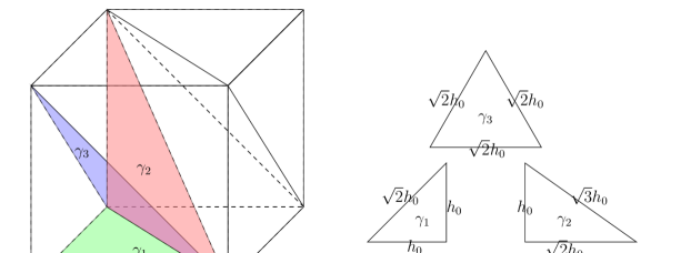
Figure 1. Mesh of type cub6 and penalty parameters on different interior faces.

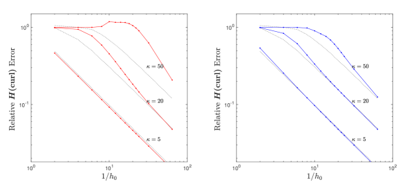
Figure 2. Log-log plots of the relative ${\bm{H}}(\operatorname{\bm{\mathrm{curl}}})$ errors of the EE solution (left), the CIP-EE solution (right), and the interpolation (black dotted line) versus $1/h_{0}$ with $1/h_{0}=2,4,\cdots,24,32$ and $64$, for $\kappa=5,20$, and $50$, respectively.

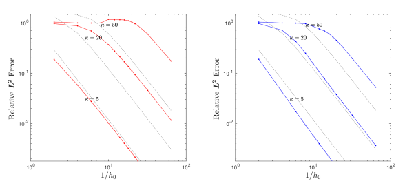
Figure 3. Log-log plots of the relative ${\bm{L}}^{2}$ errors of the EE solution (left), the CIP-EE solution (right), and the interpolation (black dotted line) versus $1/h_{0}$ with $1/h_{0}=2,4,\cdots,24,32$ and $64$, for $\kappa=5,20$, and $50$, respectively.

Figures 2 and 3 illustrate the relative ${\bm{H}}(\operatorname{\bm{\mathrm{curl}}})$ errors and the relative ${\bm{L}}^{2}$ errors of the EE solutions (left), the CIP-EE solutions (right), and the interpolations (black dot line) for $\kappa=5$, $20$, and $50$, respectively. It demonstrates that when $\kappa=5$, the errors of the solutions to EEM and CIP-EEM closely match those of the corresponding EE interpolations, implying the absence of pollution errors for small wave numbers. Conversely, for large $\kappa$, the relative errors of the EE solutions decay slowly, starting from a point considerably distant from the decaying point of the corresponding EEM interpolations. This behavior vividly exposes the presence of pollution errors in the EEM. The CIP-EE solutions exhibit a similar behavior to the EE solutions, but the pollution range of the former is significantly smaller than that of the latter.

Figure 4 presents plots of relative ${\bm{H}}(\operatorname{\bm{\mathrm{curl}}})$ errors with mesh constraint $\kappa h_{0}=1$ for EEM and CIP-EEM with $\kappa=1,2,\cdots,100$, respectively. Note that for small wave number $\kappa$, the errors of EE and CIP-EE solutions closely match those of the corresponding EE interpolations, implying that pollution errors do not manifest for small wave numbers. For large values of $\kappa$, the relative errors of EE solutions deteriorate rapidly. This behavior clearly demonstrates the impact of the pollution error in the EEM. The CIP-EE solutions behave well till $\kappa=100$, which shows the pollution effect for this method is significantly smaller than that of the EEM.

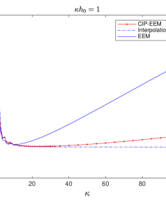
Figure 4. Relative ${\bm{H}}(\operatorname{\bm{\mathrm{curl}}})$ errors with $\kappa h_{0}=1$.

Appendix: Proof of Lemma 3.2

Denote by $\pi_{N}$ the interpolation onto the second-type Nédélec edge element space $\bm{V}_{h}$. The following lemma gives the interpolation error estimates.

Lemma A.1.

We have

$$\|\operatorname{\bm{\mathrm{curl}}}({\bm{u}}-\pi_{N}{\bm{u}})\|\lesssim h|{\operatorname{\bm{\mathrm{curl}}}\bm{u}}|_{1},$$ (A.1)

$$\|{\bm{u}}-\pi_{N}{\bm{u}}\|\lesssim h^{2}|{\bm{u}}|_{2},$$ (A.2)

$$\|({\bm{u}}-\pi_{N}{\bm{u}})_{T}\|_{\Gamma}\lesssim h^{\frac{3}{2}}|{\bm{u}}|_{2},$$ (A.3)

$$\interleave{\bm{u}}-\pi_{N}{\bm{u}}\interleave\lesssim h|{\operatorname{\bm{\mathrm{curl}}}\bm{u}}|_{1}+C_{\kappa h}(\kappa h)^{\frac{1}{2}}h|{\bm{u}}|_{2}.$$ (A.4)

Proof.

For (A.1)–(A.2), we refer to [31, Theorems 8.15, 5.41]. The estimate (A.3) follows from the local trace inequality and (A.4) follows from (A.1)–(A.3). The proof is completed. ∎

Without loss of generality, we prove Lemma 3.2 only for $\tilde{{\bm{u}}}_{h}:=P_{h}^{+}\bm{u}$. The proof of (3.10a) is obvious and is omitted. Next we prove (3.10b) and (3.10c).

The following lemma gives an estimate of $\|({\bm{u}}-\tilde{\bm{u}}_{h})_{T}\|_{\Gamma}$.

Lemma A.2.

It holds

$$\|({\bm{u}}-\tilde{\bm{u}}_{h})_{T}\|_{\Gamma}\lesssim\|({\bm{u}}-{\bm{v}}_{h})_{T}\|_{\Gamma}+C_{\kappa h}\big{(}h^{-\frac{1}{2}}\|{\bm{u}}-{\bm{v}}_{h}\|+h^{\frac{1}{2}}\interleave{\bm{u}}-{\bm{v}}_{h}\interleave\big{)}\quad\forall\bm{v}_{h}\in\bm{V}_{h}.$$ (A.5)

Proof.

Let ${\bm{\Phi}}_{h}:=\tilde{{\bm{u}}}_{h}-{\bm{v}}_{h}\in\bm{V}_{h}$. Similar to Lemma 3.4, we have the following decompositions (see, e.g., [31, Remark 3.46, Lemma 7.6]):

$${\bm{\Phi}}_{h}=\nabla r+{\bm{w}}=\nabla r_{h}+{\bm{w}}_{h},$$ (A.6)

where $r\in H^{1}(\Omega)$, $r_{h}\in U_{h}$, ${\bm{w}}\in{\bm{H}}^{1}(\Omega)$, and ${\bm{w}}_{h}\in\bm{V}_{h}$, ${\bm{w}}$ is divergence-free in $\Omega$, ${\bm{w}}\cdot\bm{\nu}=0$ on $\Gamma$, and there also holds

$$\|{\bm{w}}-{\bm{w}}_{h}\|\lesssim h\|{\operatorname{\bm{\mathrm{curl}}}}\ {\bm{\Phi}}_{h}\|\lesssim h\interleave{\bm{u}}-{\bm{v}}_{h}\interleave,$$ (A.7)

where we have used (3.10a) to derive the last inequality.

Next, we establish a relationship between $\|({\bm{u}}-\tilde{\bm{u}}_{h})_{T}\|_{\Gamma}$ and $\|{\bm{w}}\|$. Denote by

$$d({\bm{u}},\bm{v}):=\kappa^{2}({\bm{u}},\bm{v})-{\bm{\mathrm{i}}}\kappa\lambda\langle{\bm{u}}_{T},\bm{v}_{T}\rangle.$$

From (3.8) and (3.9), we have

$$d({\bm{u}}-\tilde{\bm{u}}_{h},\nabla r_{h})=\hat{a}({\bm{u}}-\tilde{\bm{u}}_{h},\nabla r_{h})=0,$$ (A.8)

which implies

$$d({\bm{u}}-\tilde{\bm{u}}_{h},{\bm{u}}-\tilde{\bm{u}}_{h})=d({\bm{u}}-\tilde{\bm{u}}_{h},{\bm{u}}-{\bm{v}}_{h}-{\bm{w}}_{h}).$$

And hence from the Cauchy’s inequality we obtain

$$\big{|}d({\bm{u}}-\tilde{\bm{u}}_{h},{\bm{u}}-\tilde{\bm{u}}_{h})\big{|}\lesssim\big{|}d({\bm{u}}-{\bm{v}}_{h}-{\bm{w}}_{h},{\bm{u}}-{\bm{v}}_{h}-{\bm{w}}_{h})\big{|},$$

which gives

$$\kappa\lambda\|({\bm{u}}-\tilde{\bm{u}}_{h})_{T}\|_{\Gamma}^{2}\leq\kappa\lambda\|({\bm{u}}-{\bm{v}}_{h})_{T}\|_{\Gamma}^{2}+\kappa\lambda\|{\bm{w}}_{h,T}\|_{\Gamma}^{2}+\kappa^{2}\|{\bm{u}}-{\bm{v}}_{h}\|^{2}+\kappa^{2}\|{\bm{w}}_{h}\|^{2}.$$

Therefore, by noting $\|{\bm{w}}_{h,T}\|_{\Gamma}\lesssim h^{-\frac{1}{2}}\|{\bm{w}}_{h}\|$ and using (A.7), we conclude that

$$\|({\bm{u}}-\tilde{\bm{u}}_{h})_{T}\|_{\Gamma}\lesssim \|({\bm{u}}-{\bm{v}}_{h})_{T}\|_{\Gamma}+\kappa^{\frac{1}{2}}\|{\bm{u}}-{\bm{v}}_{h}\|$$

$$+C_{\kappa h}\big{(}h^{-\frac{1}{2}}\|{\bm{w}}\|+h^{\frac{1}{2}}\interleave{\bm{u}}-{\bm{v}}_{h}\interleave\big{)}.$$ (A.9)

We utilize the duality argument to estimate $\|{\bm{w}}\|$, first we begin by introducing the dual problem:

$${\operatorname{\bm{\mathrm{curl}}}}\,{\operatorname{\bm{\mathrm{curl}}}}\,{\bm{z}}+\kappa^{2}{\bm{z}} ={\bm{w}}\qquad {\rm in}\ \Omega,$$ (A.10)

$${\operatorname{\bm{\mathrm{curl}}}}\,{\bm{z}}\times\bm{\nu}+{\bm{\mathrm{i}}}\kappa\lambda{\bm{z}}_{T} =\bm{0}\qquad {\rm on}\ \Gamma,$$ (A.11)

or in the variational form:

$$\hat{a}(\bm{v},\bm{z})=(\bm{v},\bm{w})\quad\forall\bm{v}\in\bm{V}.$$ (A.12)

Noting that ${\bm{w}}\cdot\bm{\nu}=0$ on $\Gamma$, similar to the proof of (3.3), we may derive the following ${\bm{H}}^{2}$ regularity estimate for the above problem:

$$\|{\bm{z}}\|_{2} \lesssim\|{\bm{w}}\|.$$ (A.13)

From (A.12), (A.4), we may deduce that

$$({\bm{u}}-\tilde{\bm{u}}_{h},{\bm{w}}) =\hat{a}({\bm{u}}-\tilde{\bm{u}}_{h},{\bm{z}}-\pi_{N}{\bm{z}})\lesssim\interleave{\bm{u}}-\tilde{\bm{u}}_{h}\interleave\interleave{\bm{z}}-\pi_{N}{\bm{z}}\interleave$$

$$\lesssim C_{\kappa h}\interleave{\bm{u}}-\tilde{\bm{u}}_{h}\interleave h|\bm{z}|_{2}\lesssim C_{\kappa h}h\interleave{\bm{u}}-\bm{v}_{h}\interleave\|\bm{w}\|.$$ (A.14)

Since $\|{\bm{w}}\|^{2}=({\bm{\Phi}}_{h},{\bm{w}})=({\bm{u}}-{\bm{v}}_{h},{\bm{w}})-({\bm{u}}-\tilde{\bm{u}}_{h},{\bm{w}}),$ we have from (A.14) that

$$\|{\bm{w}}\|\lesssim\|{\bm{u}}-{\bm{v}}_{h}\|+C_{\kappa h}h\interleave{\bm{u}}-{\bm{v}}_{h}\interleave,$$ (A.15)

which together with (Proof.) completes the proof of the lemma. ∎

The following lemma gives an estimate of $\|{\bm{u}}-\tilde{{\bm{u}}}_{h}\|$.

Lemma A.3.

We have

$$\|{\bm{u}}-\tilde{{\bm{u}}}_{h}\|\lesssim C_{\kappa h}\big{(}\|{\bm{u}}-{\bm{v}}_{h}\|+h\interleave{\bm{u}}-{\bm{v}}_{h}\interleave+h^{\frac{1}{2}}\|({\bm{u}}-{\bm{v}}_{h})_{T}\|_{\Gamma}\big{)}\quad\forall\bm{v}_{h}\in\bm{V}_{h}.$$ (A.16)

Proof.

The idea is to convert the estimation of $\|{\bm{u}}-\tilde{{\bm{u}}}_{h}\|$ to that of $\|({\bm{u}}-\tilde{\bm{u}}_{h})_{T}\|_{\Gamma}$. For ${\bm{\Phi}}_{h}=\tilde{{\bm{u}}}_{h}-{\bm{v}}_{h}$, according to Lemma 3.3, there exists ${\bm{\Phi}}_{h}^{c}\in\bm{V}_{h}^{0}$ such that

$$\|{\bm{\Phi}}_{h}-{\bm{\Phi}}_{h}^{c}\|+h\|{\operatorname{\bm{\mathrm{curl}}}\,}({\bm{\Phi}}_{h}-{\bm{\Phi}}_{h}^{c})\| \lesssim h^{\frac{1}{2}}\|{\bm{\Phi}}_{h,T}\|_{\Gamma}.$$ (A.17)

From Lemma 3.4 we have the following discrete Helmholtz decomposition for ${\bm{\Phi}}_{h}^{c}$:

$${\bm{\Phi}}_{h}^{c}={\bm{w}}_{h}^{0}+\nabla r_{h}^{0},$$

where $r_{h}^{0}\in U_{h}^{0}$ and ${\bm{w}}_{h}^{0}\in\bm{V}_{h}^{0}$ is discrete divergence-free. Moreover, there exists ${\bm{w}}^{0}\in{\bm{H}}_{0}({\operatorname{\bm{\mathrm{curl}}}})$ such that $\operatorname{\bm{\mathrm{div}}}{\bm{w}}^{0}=0$, $\operatorname{\bm{\mathrm{curl}}}w^{0}=\operatorname{\bm{\mathrm{curl}}}{\bm{\Phi}}_{h}^{c}$, and

$$\|{\bm{w}}_{h}^{0}-{\bm{w}}^{0}\|\lesssim h\|{\operatorname{\bm{\mathrm{curl}}}}\,{\bm{w}}_{h}^{0}\|=h\|{\operatorname{\bm{\mathrm{curl}}}}\,{\bm{\Phi}}_{h}^{c}\|.$$ (A.18)

From (3.9), we know that

$$({\bm{u}}-\tilde{\bm{u}}_{h},\nabla\phi_{h}^{0})=0\quad\forall\phi_{h}^{0}\in U_{h}^{0}.$$ (A.19)

Next, we introduce the following dual problem

$${\operatorname{\bm{\mathrm{curl}}}}\,{\operatorname{\bm{\mathrm{curl}}}}\,{{\bm{\Psi}}}+\kappa^{2}{{\bm{\Psi}}} ={\bm{w}}^{0}\quad {\rm in}\ \Omega,$$ (A.20)

$${\operatorname{\bm{\mathrm{curl}}}}\,{{\bm{\Psi}}}\times\bm{\nu}+{\bm{\mathrm{i}}}\kappa\lambda{{\bm{\Psi}}}_{T} =\bm{0}\quad {\rm on}\ \Gamma,$$ (A.21)

or in the variational form:

$$\hat{a}(\bm{v},\bm{\Psi})=(\bm{v},\bm{w}^{0})\quad\forall\bm{v}\in\bm{V}.$$ (A.22)

Similar to the proof of Lemma 3.1 (see also [29, Theorem 4.3]), we have the following estimates:

$$\|{\bm{\Psi}}\|_{{\bm{H}}^{1}(\operatorname{\bm{\mathrm{curl}}})} \lesssim\|{\bm{w}}^{0}\|,$$ (A.23)

$$\|{\bm{\Psi}}\|_{2} \lesssim\|{\bm{w}}^{0}\|+\kappa^{-1}\|{\bm{w}}^{0}\|_{1}\lesssim\|{\bm{w}}^{0}\|+\kappa^{-1}\|\operatorname{\bm{\mathrm{curl}}}{\bm{w}}^{0}\|$$

$$=\|{\bm{w}}^{0}\|+\kappa^{-1}\|{\operatorname{\bm{\mathrm{curl}}}}\,{\bm{\Phi}}_{h}^{c}\|.$$ (A.24)

Using (A.22), we obtain

$$({\bm{u}}-\tilde{\bm{u}}_{h},{\bm{w}}^{0})=\hat{a}({\bm{u}}-\tilde{\bm{u}}_{h},{\bm{\Psi}})=\hat{a}({\bm{u}}-\tilde{\bm{u}}_{h},{\bm{\Psi}}-\pi_{N}\bm{\Psi}).$$ (A.25)

Using (A.23)–(A.25) and Lemma A.1, we conclude that

$$\big{|}({\bm{u}}-\tilde{\bm{u}}_{h},{\bm{w}}^{0})\big{|}\lesssim\interleave{\bm{u}}-\tilde{\bm{u}}_{h}\interleave h|{\bm{\Psi}}|_{{\bm{H}}^{1}(\operatorname{\bm{\mathrm{curl}}})}+\big{(}\kappa^{2}h^{2}\|{\bm{u}}-\tilde{\bm{u}}_{h}\|+\kappa h^{\frac{3}{2}}\|({\bm{u}}-\tilde{\bm{u}}_{h})_{T}\|_{\Gamma}\big{)}|{\bm{\Psi}}|_{2}$$

$$\lesssim C_{\kappa h}h\interleave{\bm{u}}-\tilde{\bm{u}}_{h}\interleave\|{\bm{w}}^{0}\|+\big{(}h^{2}\interleave{\bm{u}}-\tilde{\bm{u}}_{h}\interleave+h^{\frac{3}{2}}\|({\bm{u}}-\tilde{\bm{u}}_{h})_{T}\|_{\Gamma}\big{)}\|{\operatorname{\bm{\mathrm{curl}}}}\,{\bm{\Phi}}_{h}^{c}\|.$$ (A.26)

From (A.19) and the orthogonality between ${\bm{w}}^{0}$ and $\nabla r_{h}^{0}$, we may get

$$\|{\bm{u}}-\tilde{\bm{u}}_{h}\|^{2}+\|{\bm{w}}^{0}\|^{2} =({\bm{u}}-\tilde{\bm{u}}_{h}+{\bm{w}}^{0},{\bm{u}}-\tilde{\bm{u}}_{h}+{\bm{w}}^{0})-2\operatorname{{Re}}({\bm{u}}-\tilde{\bm{u}}_{h},{\bm{w}}^{0})$$

$$=({\bm{u}}-\tilde{\bm{u}}_{h}+{\bm{w}}^{0},{\bm{u}}-{\bm{v}}_{h})-({\bm{u}}-\tilde{\bm{u}}_{h}+{\bm{w}}^{0},{\bm{\Phi}}_{h}-{\bm{\Phi}}_{h}^{c})$$

$$\quad-({\bm{u}}-\tilde{\bm{u}}_{h}+{\bm{w}}^{0},{\bm{w}}_{h}^{0}-{\bm{w}}^{0})-2\operatorname{{Re}}({\bm{u}}-\tilde{\bm{u}}_{h},{\bm{w}}^{0}),$$

which together with (Proof.) and the Young’s inequality, gives

$$\|{\bm{u}}-\tilde{\bm{u}}_{h}\|^{2}+\|{\bm{w}}^{0}\|^{2} \lesssim\|{\bm{u}}-{\bm{v}}_{h}\|^{2}+\|{\bm{\Phi}}_{h}-{\bm{\Phi}}_{h}^{c}\|^{2}+\|{\bm{w}}_{h}^{0}-{\bm{w}}^{0}\|^{2}$$

$$\quad+C_{\kappa h}h^{2}\interleave{\bm{u}}-\tilde{\bm{u}}_{h}\interleave^{2}+h\|({\bm{u}}-\tilde{\bm{u}}_{h})_{T}\|_{\Gamma}^{2}+h^{2}\|{\operatorname{\bm{\mathrm{curl}}}}\,{\bm{\Phi}}_{h}^{c}\|^{2}.$$

By (3.10a), (A.17) and (A.18), we have

$$\|{\bm{u}}-\tilde{\bm{u}}_{h}\|+\|{\bm{w}}^{0}\| \lesssim\|{\bm{u}}-{\bm{v}}_{h}\|+h^{\frac{1}{2}}\|{\bm{\Phi}}_{h,T}\|_{\Gamma}+h\|{\operatorname{\bm{\mathrm{curl}}}}\,{\bm{\Phi}}_{h}^{c}\|$$

$$\quad+C_{\kappa h}h\interleave{\bm{u}}-{\bm{v}}_{h}\interleave+h^{\frac{1}{2}}\|({\bm{u}}-\tilde{\bm{u}}_{h})_{T}\|_{\Gamma}.$$ (A.27)

From (A.17) and (3.10a) we have

$$h\|{\operatorname{\bm{\mathrm{curl}}}}\,{\bm{\Phi}}_{h}^{c}\| \leq h\|{\operatorname{\bm{\mathrm{curl}}}}\,({\bm{\Phi}}_{h}-{\bm{\Phi}}_{h}^{c})\|+h\|{\operatorname{\bm{\mathrm{curl}}}}\,{\bm{\Phi}}_{h}\|\lesssim h^{\frac{1}{2}}\|{\bm{\Phi}}_{h,T}\|_{\Gamma}+h\interleave{\bm{u}}-{\bm{v}}_{h}\interleave.$$

While using the triangle inequality, we get

$$h^{\frac{1}{2}}\|{\bm{\Phi}}_{h,T}\|_{\Gamma} \leq h^{\frac{1}{2}}\big{(}\|({\bm{u}}-\tilde{\bm{u}}_{h})_{T}\|_{\Gamma}+\|({\bm{u}}-{\bm{v}}_{h})_{T}\|_{\Gamma}\big{)}.$$

Inserting the above two inequalities into (A.27), we obtain

$$\|{\bm{u}}-\tilde{{\bm{u}}}_{h}\|\lesssim h^{\frac{1}{2}}\|({\bm{u}}-\tilde{\bm{u}}_{h})_{T}\|_{\Gamma}+h^{\frac{1}{2}}\|({\bm{u}}-{\bm{v}}_{h})_{T}\|_{\Gamma}+\|{\bm{u}}-{\bm{v}}_{h}\|$$

$$+C_{\kappa h}h\interleave{\bm{u}}-{\bm{v}}_{h}\interleave\quad\forall\bm{v}_{h}\in\bm{V}_{h},$$ (A.28)

which together with Lemma A.2 completes the proof of the lemma. ∎

Finally, the proof of Lemma 3.2 follows by taking $\bm{v}_{h}=\pi_{N}{\bm{u}}$ in Lemmas A.2–A.3 and using Lemma A.1. ∎

References

- [1] R. A. Adams and J. J. Fournier. Sobolev spaces. Elsevier, 2003.
- [2] M. Ainsworth. Discrete dispersion relation for -version finite element approximation at high wave number. SIAM Journal on Numerical Analysis, 42(2):553–575, 2004.
- [3] M. Ainsworth. Dispersive properties of high–order Nédélec/edge element approximation of the time–harmonic Maxwell equations. Philosophical Transactions of the Royal Society of London. Series A: Mathematical, Physical and Engineering Sciences, 362(1816):471–491, 2004.
- [4] C. Amrouche, C. Bernardi, M. Dauge, and V. Girault. Vector potentials in three-dimensional non-smooth domains. Mathematical Methods in the Applied Sciences, 21(9):823–864, 1998.
- [5] I. M. Babuška and S. A. Sauter. Is the pollution effect of the FEM avoidable for the Helmholtz equation considering high wave numbers? SIAM Journal on Numerical Analysis, 34(6):2392–2423, 1997.
- [6] S. Brenner and L. Scott. The mathematical theory of finite element methods. Springer, 2008.
- [7] E. Burman. A unified analysis for conforming and nonconforming stabilized finite element methods using interior penalty. SIAM Journal on Numerical Analysis, 43(5):2012–2033, 2005.
- [8] E. Burman, H. Wu, and L. Zhu. Linear continuous interior penalty finite element method for Helmholtz equation with high wave number: One-dimensional analysis. Numerical Methods for Partial Differential Equations, pages 1378–1410, 2016.
- [9] Z. Chen. On the regularity of time-harmonic Maxwell equations with impedance boundary conditions. Commun. Appl. Math. Comput., 2024.
- [10] D. L. Colton, R. Kress, and R. Kress. Inverse acoustic and electromagnetic scattering theory, volume 93. Springer, 1998.
- [11] M. Costabel, M. Dauge, and S. Nicaise. Corner Singularities and Analytic Regularity for Linear Elliptic Systems. Part I: Smooth domains. 211 pages, Feb. 2010.
- [12] J. Douglas and T. Dupont. Interior penalty procedures for elliptic and parabolic Galerkin methods. In Computing Methods in Applied Sciences: Second International Symposium December 15–19, 1975, pages 207–216. Springer, 2008.
- [13] Y. Du and H. Wu. Preasymptotic error analysis of higher order FEM and CIP-FEM for Helmholtz equation with high wave number. SIAM Journal on Numerical Analysis, 53(2):782–804, 2015.
- [14] X. Feng, P. Lu, and X. Xu. A hybridizable discontinuous Galerkin method for the time-harmonic Maxwell equations with high wave number. Computational Methods in Applied Mathematics, 16(3):429–445, 2016.
- [15] X. Feng and H. Wu. -discontinuous Galerkin methods for the Helmholtz equation with large wave number. Math. Comp., 80(276):1997–2024, 2011.
- [16] X. Feng and H. Wu. An absolutely stable discontinuous Galerkin method for the indefinite time-harmonic Maxwell equations with large wave number. SIAM Journal on Numerical Analysis, 52(5):2356–2380, 2014.
- [17] G. N. Gatica and S. Meddahi. Finite element analysis of a time harmonic Maxwell problem with an impedance boundary condition. IMA Journal of Numerical Analysis, 32(2):534–552, 2012.
- [18] R. Hiptmair. Finite elements in computational electromagnetism. Acta Numerica, 11:237–339, 2002.
- [19] R. Hiptmair, A. Moiola, and I. Perugia. Stability results for the time-harmonic Maxwell equations with impedance boundary conditions. Mathematical Models and Methods in Applied Sciences, 21:2263–2287, 2011.
- [20] R. Hiptmair, A. Moiola, and I. Perugia. Error analysis of Trefftz-discontinuous Galerkin methods for the time-harmonic Maxwell equations. Mathematics of Computation, 82(281):247–268, 2013.
- [21] P. Houston, I. Perugia, A. Schneebeli, and D. Schötzau. Interior penalty method for the indefinite time-harmonic maxwell equations. Numerische Mathematik, 100:485–518, 2005.
- [22] F. Ihlenburg. Finite element analysis of acoustic scattering, volume 132 of Applied Mathematical Sciences. Springer-Verlag, New York, 1998.
- [23] J.-M. Jin. Theory and computation of electromagnetic fields. John Wiley & Sons, 2015.
- [24] P. Lu, H. Chen, and W. Qiu. An absolutely stable -HDG method for the time-harmonic Maxwell equations with high wave number. Mathematics of Computation, 86(306):1553–1577, 2017.
- [25] P. Lu, Y. Wang, and X. Xu. Regularity results for the time-harmonic Maxwell equations with impedance boundary condition. arXiv:1804.07856v1, 2018.
- [26] P. Lu, H. Wu, and X. Xu. Continuous interior penalty finite element methods for the time-harmonic Maxwell equation with high wave number. Adv. Comput. Math., 45(5–6):3265–3291, dec 2019.
- [27] J. M. Melenk and S. Sauter. Convergence analysis for finite element discretizations of the Helmholtz equation with Dirichlet-to-Neumann boundary conditions. Mathematics of Computation, 79(272):1871–1914, 2010.
- [28] J. M. Melenk and S. Sauter. Wavenumber explicit convergence analysis for Galerkin discretizations of the Helmholtz equation. SIAM Journal on Numerical Analysis, 49(3):1210–1243, 2011.
- [29] J. M. Melenk and S. A. Sauter. Wavenumber-explicit -FEM analysis for Maxwell’s equations with transparent boundary conditions. Foundations of Computational Mathematics, 21(1):125–241, 2020.
- [30] J. M. Melenk and S. A. Sauter. Wavenumber-explicit -FEM analysis for Maxwell’s equations with impedance boundary conditions. Foundations of Computational Mathematics, 2023.
- [31] P. Monk et al. Finite element methods for Maxwell’s equations. Oxford University Press, 2003.
- [32] P. B. Monk and A. K. Parrott. A dispersion analysis of finite element methods for Maxwell’s equations. SIAM Journal on Scientific Computing, pages 916–937, 1994.
- [33] D. J. Naylor. Filling space with tetrahedra. International Journal for Numerical Methods in Engineering, 44(10):1383–1395, 1999.
- [34] J. C. Nédélec. Mixed finite elements in . Numer. Math., 35(3):315–341, sep 1980.
- [35] J. C. Nédélec. A new family of mixed finite elements in . Numer. Math., 50(1):57–81, nov 1986.
- [36] S. Nicaise and J. Tomezyk. The time-harmonic Maxwell equations with impedance boundary conditions in polyhedral domains, pages 285–340. De Gruyter, Berlin, Boston, 2019.
- [37] S. Nicaise and J. Tomezyk. Convergence analysis of a -finite element approximation of the time-harmonic Maxwell equations with impedance boundary conditions in domains with an analytic boundary. Numerical Methods for Partial Differential Equations, 36(6):1868–1903, 2020.
- [38] O. Schenk, K. Gärtner, W. Fichtner, and A. D. Stricker. PARDISO: a high-performance serial and parallel sparse linear solver in semiconductor device simulation. Future Gener. Comput. Syst., 18:69–78, 2001.
- [39] H. Wu. Pre-asymptotic error analysis of CIP-FEM and FEM for the Helmholtz equation with high wave number. Part I: linear version. IMA Journal of Numerical Analysis, 34:1266–1288, 2014.
- [40] H. Wu. FEM and CIP-FEM for Helmholtz equation with high wave number (in Chinese). Mathematica Numerica Sinica, 40:191–213, 2018.
- [41] Y. Zhou. Dispersion analysis of CIP-FEM for Helmholtz problem. PhD thesis, Nanjing University, 2023.
- [42] Y. Zhou and H. Wu. Dispersion analysis of CIP-FEM for the Helmholtz equation. SIAM Journal on Numerical Analysis, 61(3):1278–1292, 2023.
- [43] B. Zhu and H. Wu. Preasymptotic error analysis of the HDG method for Helmholtz equation with large wave number. Journal of scientific computing, pages 63(1–34), 2021.
- [44] L. Zhu and H. Wu. Preasymptotic error analysis of CIP-FEM and FEM for Helmholtz equation with high wave number. Part II: version. SIAM Journal on Numerical Analysis, 51(3):1828–1852, 2013.