Fuzzy Color Model and Clustering Algorithm for Color Clustering Problem

Abstract: The research interest of this paper is focused on the efficient clustering task for an arbitrary color data. In order to tackle this problem, we have tried to model the inherent uncertainty and vagueness of color data using fuzzy color model. By taking fuzzy approach to color modeling, we could make a soft decision for the vague regions between neighboring colors. The proposed fuzzy color model defined a three dimensional fuzzy color ball and color membership computation method with two inter-color distances. With the fuzzy color model, we developed a new fuzzy clustering algorithm for an efficient partition of color data. Each fuzzy cluster set has a cluster prototype which is represented by fuzzy color centroid.

I. Introduction

Color is the one of the most important features in our lives. It is not easy task to effectively describe color in our language even though color can be considered as a simple and intuitive object [10][12][23]. The research interest of this paper is focused on the color clustering problem. For a given set of color data and the number of clusters, the objective is to partition the color set into homogenous color sub-partition. This kind of color clustering task can be widely used for a variety of applications, for example, color image segmentation. The difficulties of this research include not only the lack of correct color model which can describe the uncertain characteristics of color, but also the lack of efficient clustering algorithm which can deal with the vague color data.

All the literatures related to color modeling including RGB, HSV, CMY, CIELAB color spaces have only handled the crisp representation of color data. However, color has inherently uncertain and vague characteristics. For the overlapping area between two major colors, the absolute color classification is not possible because it mainly depends on both the visual decision of the observer and the surrounding color effects. Thus we have tried to develop a new color model that can represent the color uncertainty and vagueness, which results in a proposed fuzzy color model. We modeled a color space with fuzzy-set theory and created a notion of three dimensional fuzzy color ball. And we proposed two color distance measures including the distance between a color element and a fuzzy color and the distance between fuzzy colors. With the distance measures, the computation method for color membership value was defined.

In order to effectively partition the color data set, fuzzy cluster analysis technique is best choice due to the ability of dealing with color uncertainty. But most of previous fuzzy clustering algorithms were designed for crisp pattern data, thus we need to develop an new algorithm that can tackle the fuzzy data clustering. We applied the proposed fuzzy color model to devise a new approach in fuzzy clustering algorithm. Color is a qualitative feature and we have to make a soft decision in color clustering activity. Thus each color cluster set is prototyped by color centroid value that is represented by fuzzy color ball. By minimizing the pre-defined evaluation criteria, we could obtain the near-optimal convergence in an iterative color clustering.

The remainder of this paper is organized as follows. Section II gives the description of background knowledge about color and previous works in cluster analysis. We describe our new fuzzy color model and its color membership computation method in section III , and the proposed fuzzy clustering algorithm with fuzzy color model is covered in section IV. Finally we conclude our remarks in section V.

II. Literature Review

2.1 Fundamental Color Spaces

In this section, we’ll cover the three fundamental color spaces, including RGB, CMY, Munsell, and CIE uniform color systems. We will briefly describe the basic concept and its color models.

2.1.1 RGB and CMY Color Spaces

RGB color space is the most simple and familiar color system we’ve ever known. Due to the basic and well-known properties, it’s used for most of color applications and follows the additive color law. The primary components of RGB space are red, green, and blue colors. By the additive color law, the secondary components are cyan, magenta, and yellow which is obtained from the mixture of the primary colors. The major problem that RGB model suffers from is a strong degree of correlation among the three components. The three values change dependently and are highly sensitive to the variation of lightness [4]. In contrast to the RGB space, CMY color space is mainly used for color reproduction industries, for example, color printing works. The major principle in CMY color system is the subtractive color law, which is the opposite of the additive law of RGB space. The major primaries are cyan, magenta, and yellow color.

2.1.2 Munsell Color Space

$Munsell$ $color$ $space$ is the most intuitive and useful to the artists and designer [10]. Every color sensation unites three qualities, defined in the Munsell system as $hue$, $value$, and $chroma$. These three components are independent of one another because each can be varied without changing the others.

$Hue$ is the component which distinguishes one color family from another, for example, red family from yellow family, or green family from blue family. There are five major color families and five minor hue families in the halfway between each major hues. All hues are arranged in a circle. This circle of hues is often called as a Munsell color wheel. $Value$ is a component by which a light color is distinguished from a dark one, namely, it is a metric for a lightness of a given color. The whole colors in the value scale have no hue which is denoted by an $N$ (neutral). The end points of value scale are true black (N 0/) and true white (N 1/). $Chroma$ is the component which expresses the strength of a color. By the chroma level, we can distinguish the vividness between two colors. A vivid color has strong chroma.

2.1.3 CIEXYZ Color Space

In 1931 CIE (International Commission on Illumination) established the colorimetry science formally. From the time CIE has comprised the essential standards and procedures of measurement that are necessary to make colorimetry a useful tool in science and technology. The CIE focused on the color gamut problem. The gamut represents the entire range of color which can be achieved in a specific device or medium. So we can easily plot the whole color gamut that can be obtained from all color mediums. However the problem CIE had noticed was that the RGB color space could not reproduce all spectral light, which means it cannot cover the whole range of color gamut. The CIE thought this happened in the process of mixing red, blue, and green primaries, which caused a negative value effect. So they transformed the RGB color space into a different set of positive color stimuli values, called CIEXYZ color space.

The transformed $XYZ$ color values are not exactly same to the original red, green, and blue, but are approximately so. The $XYZ$ tristimulus values are just used for defining a color. But unfortunately, we can not use this as the means for calculating color difference formula and establishing human perception model because CIEXYZ color is not uniform space. We can find that colors of equal amounts of difference appear farther apart in green part of the diagram rather than they do in the red or violet part. To resolve the problem of non-uniform color scaling, CIE defined two different uniform diagrams : CIELUV color space and CIELAB color space.

2.1.4 CIELAB (1976) Color Space

A CIELAB color space is the second uniform space adopted by CIE in 1976 which showed a better uniform-scaling. The CIELAB space was based on the opponent color system, which mentioned the discoveries in the mid-1960s that somewhere between the optical nerve and the brain, retinal color stimuli are translated into distinctions between light and dark, red and green, and blue and yellow. That means a color can’t be both red and green, or both blue and yellow, because these colors oppose each other. [1]. These opponent colors are translated to CIELAB $L^{*}a^{*}b^{*}$ values. The $L^{*}$ value is the same as one of CIE $L^{*}u^{*}v^{*}$ color space. Based on the opponent theory, two axes in $a^{*}b^{*}$ space represent each opponent colors. On the $a^{*}$ axis, positive $a^{*}$-value indicates amounts of red while negative $a^{*}$-value stands for the strength of green. In similar way, On the $b^{*}$ axis, positive $b^{*}$-value indicates amounts of yellow while negative $b^{*}$-value represents the blueness. For both axes, zero is neutral gray which in $L^{*}$ axis.

The mathematical formula that calculates three $L^{*},a^{*},b^{*}$ values is defined as equation 1 [19].

$$\begin{array}[]{l}L^{*}=116(Y/Y_{n})^{1/3}-16\\ a^{*}=500[(X/X_{n})^{1/3}-(Y/Y_{n})^{1/3}]\\ b^{*}=200[(Y/Y_{n})^{1/3}-(Z/Z_{n})^{1/3}]\end{array}$$ (1)

with the constraint that $X/X_{n}$,$Y/Y_{n}$,$Z/Z_{n}>0.01$.

2.1.5 Fuzzy approach to color modeling

Vertan, one of the pioneers in fuzzy color modeling, focused on image processing problem [24]. He is interested in the imprecision and vagueness problem in digital image representation. He said that noise, quantization and sampling errors, the tolerance of the human visual system are the reasons of that problem. He associated to each color $c$, that usually is a point in the three-dimensional color gamut $C$, $\mu:C\rightarrow[0,1]$ that measures the membership degree of any color $c\prime$ from $C$ within the class color $c$. Thus, $\mu_{c}(c\prime)$ is a scalar within $[0,1]$ that expresses how similar is the color $c\prime$ with respect to the color $c$.

The fuzzy membership computation model proposed by Vertan is

$$\mu_{c}(c\prime)=\left\{\begin{array}[]{lr}1.0~{}~{}~{}~{}~{}~{}~{}~{}~{}~{}~{}~{}~{}~{}~{}~{}~{}~{}~{}~{}~{}~{}~{}~{}~{}~{}~{}~{}~{}~{}\mbox{if}~{}~{}d(c,c\prime)\leq JND\\ max(0,1.0-\frac{d(c,c\prime)}{\sigma JND})~{}~{}~{}~{}~{}~{}~{}\mbox{if}~{}~{}d(c,c\prime)>JND\\ \end{array}\right.$$ (2)

In the above equation, JND is the just noticeable color difference for the CIELAB color space, and $\sigma$ is a tuning parameter to modify the inter-color confusion.

2.2 Color Data Clustering

2.2.1 Clustering Task

Data clustering or cluster analysis organizes a collection of data patterns which is usually represented as a vector of measurements or a point in a multidimensional space into clusters based on a kind of similarity measure[7]. In contrast to discriminant analysis (or supervised classification), the clustering task (often called an unsupervised classification) classifies a given collection of unlabeled data into homogeneous groups without any labeled patterns. All useful information is obtained from the data itself. Clustering is a useful methodology in various computer science field including decision-making, machine-learning, data mining, document retrieval, image segmentation, and pattern classification. Especially, it is very meaningful in that there is little prior information available about the data. Most of clustering research to deal with color data, especially in color image segmentation, have handled the color as a general crisp element without the consideration of uncertainty and vagueness. Thus, popular clustering algorithms with a conventional color, e.g. RGB color element, represented in crisp color space have been just used.

The most intuitive and frequently used clustering algorithm is partitional algorithm (often called K-Means algorithm). A partitional clustering algorithm obtains a single partition of the data in each iteration. The time and space complexities of the partitional algorithms are typically lower than those of the hierarchical-based algorithms (single-linkage and complete-linkage algorithm) where two clusters are merged to form a larger cluster based on minimum distance criteria. Thus, the partitional algorithm has advantages in applications involving large data sets, e.g. image segmentation, for which the construction of a hierarchical linkage is computationally prohibitive [7].

The evaluation function of K-Means algorithm uses the squared error criterion, which tends to work well with isolated and compact clusters. The squared error for a clustering of a pattern set $X$ (containing $c$ clusters) is

$$e^{2}(X)=\sum_{i=1}^{c}\sum_{j=1}^{n}(\|x_{j}^{i}-v_{i}\|)^{2}$$ (3)

where $n$ is the number of data $x\in X$, and $x_{j}^{i}$ is the $j^{th}$ pattern belonging to the $i^{th}$ cluster and $v_{i}$ is the centroid of the $i^{th}$ cluster. The minimization of the evaluation function generates a well-partitioned data collection. However this is sensitive to the selection of the initial partition and may converge to a local minimum of the criterion function value if the initial partition is not properly chosen.

2.2.2 Fuzzy Clustering Algorithm

The fuzzy clustering algorithm (often called FCM) generates a fuzzy partition providing a measure of membership degree $\mu_{i}$ of each data $x_{i}$ to a given cluster $c_{i}$. The formal description on Bezdek’s fuzzy clustering algorithm is as follows. For given data $x_{1},...,x_{n}\in X$ where each $x_{j}$ is a $p$-dimensional real-valued vector for all $k\in{1,...,n}$. The goal is to find a partition or cluster of $c$ fuzzy sets $F_{i},i=1,...,c$. The objective is to assign memberships in each of the fuzzy sets so that the data are strongly associated within each cluster but only weakly associated between different clusters. Each cluster is defined by its centroid, $v_{i}$, which can be calculated as a function of the fuzzy memberships of all the available data for the cluster.

The evaluation function ($J$) of fuzzy clustering looks like

$$J_{m}(F)=\sum_{i=1}^{c}\sum_{j=1}^{n}[F_{i}(x_{j})]^{m}\|x_{j}-v_{i}\|^{2}$$ (4)

where $\|\cdot\|$ is an inner product norm in $\Re^{p}$ and $\|x_{j}-v_{j}\|^{2}$ is a distance between $x_{k}$ and $v_{i}$. The objective is to minimize $J_{m}(F)$ for some set of clusters $F$ and chosen value of $m$. The parameter $m>1$ controls the influence of the fuzzy membership of each datum. The choice of $m$ is subjective, however, many applications are performed using $m=2$. That is, the goal is to iteratively improve a sequence of sets of fuzzy clusters $F(1),F(2),...$ until a set $F(t)$ is found such that no further improvement in $J_{m}(F)$ is possible. In general, the design of membership functions is the most important problem [13].

The advantages of fuzzy clustering algorithms can be summarized like this [17]. First, fuzzy clustering approach is less prone to local minima than crisp clustering algorithms since they make soft decisions in each iteration through the use of membership functions. Second, the use of the fuzzy sets allows us to manage uncertainty on measures, lack of information, …, all characteristics which bring ambiguity notions. Finally, in various fields, such as pattern recognition, data analysis and image processing, FCM is very robust and obtains good results in many clustering problems. The algorithm provides an iterative clustering of the search space and does not require any initial knowledge about the structure in the data set.

2.3 Limitations of Previous Research

2.3.1 Lack of Color Uncertainty Representation

One of the major factors affecting color description is that color depends on neighboring color stimuli in the observer’s visual field. Cognitive scientists explain this results from the interactions between cone receptors in the retina. These phenomena are called ”simultaneous contrast” or ”chromatic induction effect” [20]. This color description can be understood by computing perceived color difference among given colors. We could easily guess that the mathematical color model which determines the color difference perceivable by different for an observer is mainly dependent on the observer. The observer may judge the color difference relatively and subjectively. This is the reason none of the many color difference formula that have been proposed in the literature over the past several decades is considered as a sufficiently adequate solution of the problem. As we can see, we cannot handle this color problem with the conventional color models. Most of color models including RGB and CIELAB persues the crisp color representation and color difference formula. The simple use of the color representation does not explain the similar perception and visual confusion of certain colors.

Even though Vertan recently proposed the fuzzy approach for color modeling, his model has also several drawbacks. One of them is there’s no notion on simultaneous contrast in his model. As already mentioned, color difference description is dependent on surrounding neighboring colors relatively. He didn’t consider neighboring effect in the membership computation. The color membership should be calculated relatively according to the surrounding neighbor colors.

2.3.2 Lack of Clustering Algorithm for Fuzzy Color Data

Most clustering algorithms are designed for treating crisp color data. The practical techniques are K-Means clustering or FCM clustering for RGB color representation. With this approach, however, we cannot handle the color uncertainty problem. Yang and Liu recently proposed a class of fuzzy c-numbers clustering procedures for fuzzy data where high-dimensional fuzzy vector data are handled [22]. But the fuzzy data with conical fuzzy vector is somewhat theoretical and is not appropriate for color representation. Thus we need to develop an fuzzy color model that can explain the color uncertainty and relative color difference formula. With the proposed color model, we developed an effective fuzzy clustering algorithm for color data.

III. Proposed Fuzzy Color Model

3.1 Research Approach

In order to solve color clustering problem, we should take the following three factors into account. The first one is a pattern representation including the number, type, and scale of the features. The second one is the definition of a inter-pattern proximity measure. The most famous measure is Euclidean distance measure. Finally we should develop an efficient clustering algorithm. In this paper, we proposed and used a new fuzzy color model as a color pattern representation method, and defined two distance metrics to solve the inter-color pattern proximity. Finally by developing fuzzy clustering algorithm with fuzzy color, we could obtain an acceptable solution.

A new fuzzy color model should be created in order to satisfy the following four conditions.

• proposed model must provide human perception-based color distance metric

• proposed model must be uniform color space

• proposed model must resolve the vague color boundaries

• proposed model must compute the color membership degree in a relative way

In order to satisfy the conditions 1 and 2, we take a CIELAB color space as a basic color coordinate. The CIELAB color space was originally developed to provide the color difference formula like human perception distance based on Munsell color description, and more, it is uniform space and covers the whole color gamut. To fulfill the conditions 3 and 4, we created a color model based on fuzzy set theory. Thus color can be described as a membership degree to a specific color, and the notion of color membership resolves the vague boundaries between colors and relative color acceptability.

3.2 Description of Fuzzy Color Model

3.2.1 Three-dimensional Fuzzy Color Ball

Fuzzy color is described with three dimensional ball-type representation. To describe color concept in three dimensional color space, sphere or ball-shaped model is preferred. In this paper, a terminology $ball$ and $sphere$ are used interchangeably. The formal definition of fuzzy color ball is described in section 3.2.3. When we look a color or colored object, for example red color, some pairs of red colors are difficult to distinguish, and beyond a certain boundary, we can easily distinguish color pairs. Color has three dimensional volume representation. The radius of color ball is the JND of each color. For a pair of two colors within JND value, we assumed it is not easy to distinguish and we consider those two colors are equal. And for colors which don’t belong to JND volume, those two colors can be distinguished.

To describe the fuzzy color ball, two numerical values should be specified: center and JND value. Center value is the center point of fuzzy color ball which is calculated from CIELAB color space and Munsell color wheel. And JND means a just noticeable distance which is the distance from the center to a boundary of a given color. Figure 1 shows a fuzzy color ball on CIELAB color space. Here we must distinguish two objects: color element and fuzzy color. Color element denoted by $x$ is a point on CIELAB color coordinates, which is represented by $(x_{L},x_{a},x_{b})$ tuple value. Fuzzy color denoted by $\tilde{c}_{i}\in\tilde{C}$ is a ball or sphere with a three dimensional volume representation on CIELAB space. By taking CIELAB as a basic color coordinates, it is no doubt that the proposed fuzzy color model has an uniform color scaling.

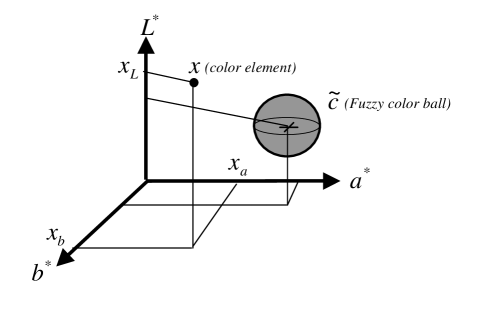
Figure 1: A Fuzzy color ball on CIELAB color space

For a given color element $x$, the membership $\mu_{\tilde{c}_{i}}(x)$ of $x$ to fuzzy color $\tilde{c}_{i}$ is obtained with the distance computation. Figure 2 depicts the fuzzy color ball and its membership function shape. In this figure, there are fuzzy color $\tilde{c}_{i}$ and color element $x$. The fuzzy color has its own center value $center_{i}$ and JND value $jnd_{i}$ that build three dimensional ball-shaped representation. If a color $x$ is within JND distance it strongly belongs to that color and has membership degree 1.0. If color $x$ is out of the range JND, the membership degree is computed relatively by comparing with neighbor colors. The left and right shape of fuzzy membership function is determined based on the distance result between fuzzy colors.

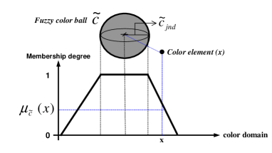
Figure 2: Fuzzy color ball and its membership shape

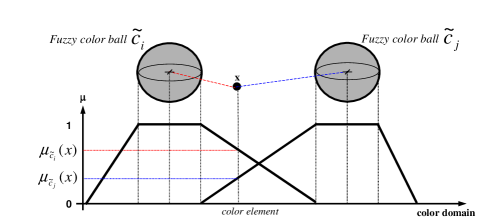
Figure 3: Membership computation among fuzzy colors

Figure 3 depicts the membership computation situation between two colors. To compute a membership degree to a specific fuzzy color, we compute all distances between fuzzy colors. If a color $x$ strongly belongs to a given color $\tilde{c}_{i}$, it is classified to that color with a membership degree $1.0$. In another case, if the color $x$ is within other color $\tilde{c}_{j}$, then it means color $x$ has no relation to the fuzzy color $\tilde{c}_{i}$, thus the membership degree to $\tilde{c}_{i}$ is $0.0$. Except the above two cases, the color $x$ is located in the middle of fuzzy colors. We compute the relative distance between fuzzy colors and detemine the membership value. And the important point is that sum of membership value to the whole fuzzy colors must be equal to 1.0. With this constraint we can easily extend this concept to fuzzy clustering algorithm.

3.2.2 Distance Measures Between Fuzzy Colors

To effectively address the new definition of fuzzy color ball and its membership computation method, we should define two inter-color distances: distance between color elements and distance between a fuzzy color and a color element.

To successfully formulate the distance between fuzzy colors, a basic color distance measure must be established between color elements.

Definition 1

Let $x$ and $y$ be two color elements on CIELAB color space, then the distance between color element $x$ and color element $y$, denoted by $\rho(x,y)$, is defined as

$$\rho(x,y)=\sqrt{(x_{L}-y_{L})^{2}+(x_{a}-y_{a})^{2}+(x_{b}-y_{b})^{2}}$$ (5)

where $x=(x_{L},x_{a},x_{b})$ and $y=(y_{L},y_{a},y_{b})$

The above definition is trivially obtained from $CIELAB$ color difference formula. Figure 4 (a) shows the distance between color elements $x$ and $y$.

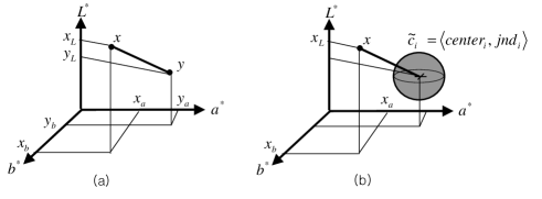
Figure 4: Distance between color elements (a) and distance between a fuzzy color and a color element (b)

One of the major concerns is to compute the distance between a fuzzy color and an arbitrary color element. With the distance measure between color elements, we can define the distance between a fuzzy color and a color element. Figure 4 (b) shows the distance between a fuzzy color $\tilde{c_{i}}$ and a color element $x$.

Definition 2

Let $\tilde{c_{i}}$ and $x$ be a fuzzy color and a color element on CIELAB color space respectively. Then the distance between fuzzy color $\tilde{c_{i}}$ and color element $x$, denoted by $\delta(\tilde{c_{i}},x)$ is defined as

$$\begin{array}[]{l}\delta(\tilde{c_{i}},x)=\|\rho(center_{i},x)\|-jnd_{i}\\[2.84544pt] =\sqrt{(center^{i}_{L}-x_{L})^{2}+(center^{i}_{a}-x_{a})^{2}+(center^{i}_{b}-x_{b})^{2}}\\[2.84544pt] \qquad\qquad-jnd_{i}\end{array}$$ (6)

where $center_{i}$ and $jnd_{i}$ are the center and JND value of fuzzy color $\tilde{c_{i}}=\langle(center^{i}_{L},center^{i}_{a},center^{i}_{b}),jnd_{i}\rangle$, and $x=(x_{L},x_{a},x_{b})$.

As can be seen in the above definition, the distance measure considers not only the center point but also JND value. With the $JND$ value, we can reflect the specific color’s characteristics. Some colors have larger JND values, and others have smaller ones on color space. For example, greenish colors have bigger volume than redish colors. Thus the adoption of JND values provides a more clear distance computation result. Look at the following figure 5. In the figure, if you compute the color distances without the notion of JND value, the three distance results from $x$ to fuzzy color ${\tilde{c}}_{red}$, ${\tilde{c}}_{blue}$, and ${\tilde{c}}_{green}$ would be equal regardless to left and right cases of the figure. However, the computation with JND value would generate different distance results for left and right side of the figure. In the figure 5 (a), the two distances $\delta({\tilde{c}}_{red},x)$ and $\delta({\tilde{c}}_{blue},x)$ are equal. In the figure 5 (b), the distance between ${\delta(\tilde{c}}_{green},x)$ is shorter than that of $\delta({\tilde{c}}_{red},x)$ due to the JND value of fuzzy color ${\tilde{c}}_{green}$ occupies a wider area on color space. Thus we can say that color element $x$ is closer to fuzzy color ${\tilde{c}}_{green}$ rather than ${\tilde{c}}_{red}$.

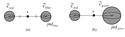
Figure 5: Distance computation of fuzzy colors with different JND value

3.2.3 Definition of Fuzzy Color Ball

With the distance computation measures defined in the above section, we can establish a formal fuzzy color model.

Definition 3

Let fuzzy color $\tilde{c}_{i}$ in a universe of discourse $\tilde{C}$ be as a three dimensional fuzzy ball set $\tilde{c_{i}}=\langle center_{i},jnd_{i}\rangle$ $\in\tilde{C}$ with a membership function such that

$$\mu_{\tilde{c_{i}}}(x)=\left\{\begin{array}[]{lr}1.0~{}~{}~{}~{}~{}~{}~{}~{}~{}~{}~{}~{}~{}~{}~{}~{}~{}~{}~{}~{}\mbox{if}~{}~{}\delta(\tilde{c_{i}},x)\leq jnd_{i}\\ 0.0~{}~{}~{}~{}~{}~{}~{}~{}~{}~{}~{}~{}~{}~{}~{}~{}~{}~{}~{}~{}\mbox{if}~{}~{}\delta(\tilde{c_{j}},x)\leq jnd_{j}\\[2.84544pt] \qquad\qquad\qquad\qquad\qquad(i\neq j,\tilde{c_{j}}\in\tilde{C})\\ (\sum_{j=1}^{|\tilde{C}|}\frac{\delta(\tilde{c_{i}},x)}{\delta(\tilde{c_{j}},x)})^{-1}~{}~{}~{}otherwise\end{array}\right.$$ (7)

where $\delta$-function means the distance between a fuzzy color and a color element.

To compute a membership degree to a specific fuzzy color, we compute all distances between fuzzy colors. If a color $x$ strongly belongs to a given fuzzy color $\tilde{c_{i}}$, it is classified to that color with a membership degree 1.0. In another case, if the color $x$ is within other fuzzy color $\tilde{c_{j}}$, then it means color $x$ has no relation to the fuzzy color $\tilde{c_{i}}$, so the membership degree is 0.0. Except the above two cases, the color $x$ is located in the middle of fuzzy colors. We compute the relative distance between fuzzy colors and determine the membership value. And the important point is that the sum of membership values to the whole fuzzy color families must be equal to 1.0. With this constraint we can easily extend this concept to fuzzy cluster analysis which is discussed in later section. The properties of the proposed fuzzy color model can be summarized as follows:

• If a color element $x$ absolutely belongs to a fuzzy color $\tilde{c_{i}}$, then $\mu_{\tilde{c_{i}}}(x)=1$.

• If a color element $x$ absolutely belongs to a fuzzy color $\tilde{c_{j}},i\neq j$, then $\mu_{\tilde{c_{i}}}(x)=0$.

• If a color element $x$ is partially related to the surrounding neighbor fuzzy colors, then $0<\mu_{\tilde{c_{i}}}(x)<1$.

• If a fuzzy color $\tilde{c_{i}}\in\tilde{C}$ is the closest fuzzy color to color element $x$, then $\mu_{\tilde{c_{i}}}(x)\geq\mu_{\tilde{c_{j}}}(x)(\forall\tilde{c}_{j}\in\tilde{C})$.

• The sum of all membership values of color element $x$ to whole fuzzy colors is equal to 1.0. ($\sum_{i=1}^{|\tilde{C}|}\mu_{\tilde{c_{i}}}(x)=1.0$)

3.2.4 Numerical Example

In this paragraph, we compute the fuzzy color distance with numerical examples. In the following examples, there are three fuzzy colors including ${\tilde{c}}_{red}$, ${\tilde{c}}_{green}$, and ${\tilde{c}}_{blue}$, and one color element $x$. We calculate the distance between fuzzy color ${\tilde{c}}_{red}$ and a given color element $x$. Let’s compute the membership degree of $x$ to fuzzy color ${\tilde{c}}_{red}$.

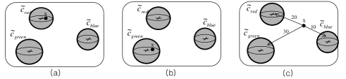
Figure 6: Numerical example of membership computation

In figure 6 (a), color element $x$ belongs to the color ${\tilde{c}}_{red}$ perfectly. In this case the membership degree $\mu_{{\tilde{c}}_{red}}(x)$ is 1.0 ($\mu_{{\tilde{c}}_{green}}(x)=0.0$ and $\mu_{{\tilde{c}}_{blue}}(x)=0.0$). In figure 6 (b), color element $x$ belongs to the color family ${\tilde{c}}_{green}$ perfectly. In this case color element $x$ has no relations to fuzzy color ${\tilde{c}}_{red}$. Thus the membership degree $\mu_{{\tilde{c}}_{red}}(x)$ is 0.0 ($\mu_{{\tilde{c}}_{green}}(x)=1.0$ and $\mu_{{\tilde{c}}_{blue}}(x)=0.0$). Look at the figure 6 (c), where color element $x$ doesn’t belong to any fuzzy colors at all, and the distances to each fuzzy color are given like this: 20 to ${\tilde{c}}_{red}$, 30 to ${\tilde{c}}_{green}$, and 10 to ${\tilde{c}}_{blue}$. In this case, we should first compute the relative strengths between fuzzy colors, and based on the strength we compute the relative color membership values. The result memberships are calculated as:

$$\mu_{{\tilde{c}}_{red}}(x)=(\frac{\delta({\tilde{c}}_{red},x)}{\delta({\tilde{c}}_{red},x)}+\frac{\delta({\tilde{c}}_{red},x)}{\delta({\tilde{c}}_{green},x)}+\frac{\delta({\tilde{c}}_{red},x)}{\delta({\tilde{c}}_{blue},x)})^{-1}$$

$$\mu_{{\tilde{c}}_{green}}(x)=(\frac{\delta({\tilde{c}}_{green},x)}{\delta({\tilde{c}}_{red},x)}+\frac{\delta({\tilde{c}}_{green},x)}{\delta({\tilde{c}}_{green},x)}+\frac{\delta({\tilde{c}}_{green},x)}{\delta({\tilde{c}}_{blue},x)})^{-1}$$

$$\mu_{{\tilde{c}}_{blue}}(x)=(\frac{\delta({\tilde{c}}_{blue},x)}{\delta({\tilde{c}}_{red},x)}+\frac{\delta({\tilde{c}}_{blue},x)}{\delta({\tilde{c}}_{green},x)}+\frac{\delta({\tilde{c}}_{blue},x)}{\delta({\tilde{c}}_{blue},x)})^{-1}$$

Thus the final membership degree of color $x$ to fuzzy colors are like this:

$$\mu_{{\tilde{c}}_{red}}(x)=(20/20+20/30+20/10)^{-1}=0.27$$

$$\mu_{{\tilde{c}}_{green}}(x)=(30/20+30/30+30/10)^{-1}=0.18$$

$$\mu_{{\tilde{c}}_{blue}}(x)=(10/20+10/30+10/10)^{-1}=0.55$$

With the result, we can say that color element $x$ is close to fuzzy color ${\tilde{c}}_{red}$ with a membership 0.27. As mentioned earlier, the membership constraint (the sum of membership to all fuzzy color families is 1.0) in examples is successfully satisfied.

IV. Fuzzy Clustering Algorithm based on Fuzzy Color Model

4.1 Problem Formulation of Color Clustering

The goal of our research is to cluster the color space represented in CIELAB color system. To accomplish this, fuzzy clustering technique is selected as a major algorithm approach because the major feature ’color’ of the data pattern has uncertain and vague properties. Thus fuzzy approach has an advantage over the hard clustering algorithms to handle these problems.

The following terms and notations are used to describe the problem formulation. The given color element data are $x_{1},...,x_{n}\in X$ where each $x_{j}$ ($j\in{1,...,n}$) is a color element represented as three-dimensional $L^{*}a^{*}b^{*}$ value on CIELAB color space. The algorithm objective is to cluster a collection of given color elements into $c$ homogeneous groups represented as fuzzy sets ($\tilde{F_{i}},i=1,...,c$) with similar color characteristics. The fuzzy cluster set can be written like an equation 8.

$$\begin{array}[]{l}\tilde{F_{i}}=\{(x_{1},\mu_{F_{i}}(x_{1}),(x_{2},\mu_{F_{i}}(x_{2}),...,(x_{n},\mu_{F_{i}}(x_{n})\}\\[2.84544pt] \,\quad=\sum_{j=1}^{n}\mu_{F_{i}}(x_{j})/x_{j}\end{array}$$ (8)

The collection of fuzzy cluster set is denoted by $\tilde{F}=\{\tilde{F_{1}},\tilde{F_{2}},..,\tilde{F_{c}}\}$. Each fuzzy cluster is defined by its centroid, denoted by $\tilde{c}_{i}$, which is represented by the proposed fuzzy color model. The pattern matrix $M$ which is handled by clustering algorithm is represented as an $c\times n$ pattern matrix. An element $p_{ij}$ in matrix $M$ means that a color element $x_{j}$ is classified to a fuzzy cluster $\tilde{F}_{i}$.

The equation 9 shows the evaluation function of the proposed approach. The objective is to minimize the evaluation function $J(\tilde{F})$ for a given pattern matrix.

$$J(\tilde{F})=\sum_{i=1}^{c}\sum_{j=1}^{n}[\mu_{\tilde{F}_{i}}(x_{j})]^{2}\delta(\tilde{c_{i}},x_{j})$$ (9)

where $\mu_{\tilde{F}_{i}}(x_{j})$ is the membership degree of color element $x_{j}$ to a fuzzy cluster set $\tilde{F}_{i}$, and $\delta(\tilde{c_{i}},x_{j})$ is the distance between the color element $x_{j}$ and the centroid $\tilde{c_{i}}$ of the fuzzy cluster set $\tilde{F}_{i}$. The goal is to iteratively improve a sequence of sets of fuzzy clusters $\tilde{F}(1),\tilde{F}(2),...$ until $\tilde{F}(t)$ is found such that no further improvement in $J(\tilde{F})$ is possible. In general, the design of membership function and centroid prototype are the most important problems. The detailed algorithm is discussed in section LABEL:sec:skeleton-of-proposed-fuzzy-clustering-algorithm.

4.2 Initialization of Cluster Analysis

Before we describe the detailed clustering algorithm, we discuss how to obtain the initial partition of color cluster set. In cluster analysis, initialization plays an important role. According to the initial starting point, the clustering algorithm might terminate at different clustering result. There is no general agreement about a good initialization scheme. Two most popular techniques are (1) using the first $c$ pattern data (2) using $c$ elements randomly from pattern set. In this paper, we propose a novel initial selection method based on the notion of fuzzy color. It is simple and intuitive.

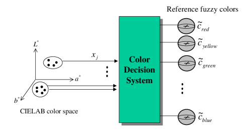
Figure 7: Initial selection of fuzzy cluster centroid

The basic idea is as follows. For a color element $x_{j}\in X$, we compute the matching degree to pre-defined thirteen reference fuzzy colors which is denoted by $\tilde{c}_{R}$. Reference fuzzy colors are selected from both the major color family in Munsell color wheel (5R, 5YR, 5Y, …, 5P, and 5RP) and the $L^{*}$-axis components (white, black, gray) of CIELAB color space. Figure 7 shows the overall initial selection process. The input of a initial color decision system is color elements in pattern space, and the output is a list of fuzzy colors where the fuzzy colors are sorted by the maximum matching score. The first $c$ fuzzy colors are chosen as the initial fuzzy cluster centroid.

For a given color element $x_{j}$, the matching score is computed by considering the membership degree $\mu_{{\tilde{c}}_{i}}(x_{j})$ to all reference fuzzy colors. Each reference fuzzy color $\tilde{c}_{i}\in\tilde{C}_{R}$ has two additional attributes denoted by $winner_{i}^{count}$ and $winner_{i}^{element}$. The $winner_{i}^{count}$ means how many color elements belong to the given reference fuzzy color $\tilde{c}_{i}$.

$$\begin{array}[]{l}winner_{i}^{count}\longleftarrow winner_{i}^{count}+1\\[2.84544pt] \qquad\qquad~{}~{}~{}~{}~{}if~{}~{}\mu_{\tilde{c}_{i}}(x_{j})\geq\mu_{\tilde{c}_{k}}(x_{j})(\forall\tilde{c}_{k}\in\tilde{C}_{R})\end{array}$$ (10)

The $winner_{i}^{element}$ is used as a center element of a newly created fuzzy color and is assigned as the color element that has maximum membership degree to this reference fuzzy color.

$$\begin{array}[]{l}winner_{i}^{element}\longleftarrow x_{j}\\[2.84544pt] \qquad~{}~{}~{}~{}~{}~{}~{}~{}~{}~{}~{}~{}~{}~{}if~{}~{}\mu_{\tilde{c}_{i}}(x_{j})\geq\mu_{\tilde{c}_{i}}(x_{k})(\forall x_{k}\in X)\end{array}$$ (11)

After the classification decision process, we build a sorted list of thirteen fuzzy colors according to their $winner_{i}^{count}$ in a descending order. From the sorted list we select the first $c$ (number of clusters) fuzzy colors which have a larger matching counter than other colors. We don’t need to focus on the whole thirteen colors in the list, just $c$ fuzzy colors are enough for the candidates for cluster centroid.

4.3 Fuzzy Clustering using Fuzzy Color

4.3.1 Fuzzy Colored Centroid Representation

The previous fuzzy clustering algorithm including FCM was designed only to deal with crisp data element. This means they can be regarded as a fuzzy clustering algorithm for crisp data. They did not consider any mechanisms about how to handle fuzzy data, especially color characteristics, even though the fuzzy clustering methodology is very appropriate to efficiently deal with the vague boundaries between fuzzy color data. Cluster analysis can be explained in the viewpoint of pattern matrix $M$. By updating the pattern matrix iteratively in each sequence step, clustering algorithm goes on the convergence condition. The typical matrix $M$ has a $c\times n$ matrix form, where each cluster centroids $c_{i}$ represent the row attribute of $M$, and each data element $x_{j}$ stands for the column of matrix. In this situation all the data elements and cluster centroids have crisp representation, thus conventional approach has a limitation to account for the uncertainty and vagueness in color clustering.

We tried to represent the fuzziness and vagueness resolution method into pattern matrix. Proposed approach is to replace the typical point-prototype crisp centroid with a new cluster centroid represented by the fuzzy color. Figure 8 depicts the skeleton of the proposed pattern matrix. The column of matrix contains each color elements $x_{j}$, and the row elements represent the centroid $\tilde{c}_{i}$ of each fuzzy cluster $\tilde{F}_{i}$ which is shown as three dimensional fuzzy color ball. Fuzzy color centroid has its own center element and JND value that are a specific properties of a given fuzzy cluster. This makes it possible to cope with the clustering decision problem in the vague region between neighbor fuzzy color clusters. With the initialization step to obtain the initial fuzzy color centroids $\tilde{c}_{i}$, the membership computation of each element $\mu_{{\tilde{F}}_{i}}(x_{j})$ in pattern matrix is carried out. The membership degree of color element $x_{j}$ to the fuzzy cluster $\tilde{F}_{i}$ is computed by the relative distance between neighbor fuzzy color centroids. After this cluster initialization process, the fuzzy color centroids and the membership degrees of matrix elements are iteratively updated until no improvements are found.

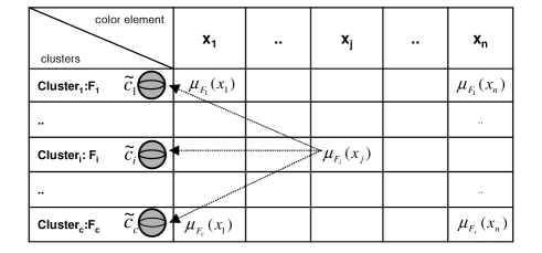
Figure 8: Membership update in proposed pattern matrix

4.3.2 Skeleton of Proposed Algorithm

As mentioned in earlier section, the objective is to obtain the optimal partition $\tilde{F}=\{\tilde{F_{1}},\tilde{F_{2}},..,\tilde{F_{c}}\}$ for a given color elements $x_{1},...,x_{n}$ and number of clusters $c$ by minimizing the evaluation function $J(\tilde{F})$. The algorithmic step can be described as followings:

Step 1.

With a given pre-determined number of clusters ($c$) and the color data elements ($x_{1},...,x_{n}\in X$), run the proposed cluster initialization method to obtain the candidates of fuzzy color centroids.

Step 2.

Create the initial $\tilde{c}$ fuzzy color centroids, $\tilde{c_{1}}(t),...,\tilde{c_{c}}(t)$ where $t$ means the iteration step (initially $t=0$) with the candidates obtained in Step 1. The newly created fuzzy color centroid $\tilde{c}_{i}$ is defined as follows:

$$\tilde{c_{i}}=\langle center_{i},jnd_{i}\rangle$$ (12)

$$center_{i}\leftarrow winner_{i}^{element}$$ (13)

$$jnd_{i}\leftarrow jnd_{k}~{}~{}s.t.~{}~{}\{k|\forall\tilde{c}_{k}\in\tilde{C}_{R},~{}min_{k}\delta(\tilde{c}_{k},center_{i})\}$$ (14)

where $\delta$-function means the distance between a color element and a fuzzy color, and $\tilde{C}_{R}$ represent the universe of discourse of the predefined thirteen reference fuzzy colors.

Step 3.

Update the membership degree of fuzzy cluster sets $\tilde{F}_{i}(t+1)$ by the following procedure. For each color element $x_{j}$:

• if $\delta(\tilde{c_{i}},x_{j})<jnd_{\tilde{c_{i}}}$, then update the membership of $x_{j}$ in $\tilde{F}_{i}$ at $t+1$ iteration by

  $$\mu_{\tilde{F}_{i}}(x_{j})(t+1)=1.0$$ (15)

• if $\delta(\tilde{c_{k}},x_{j})<jnd_{\tilde{c_{k}}}$, for $k\neq i,\tilde{c}_{k}\in\tilde{C}$ then update the membership of $x_{j}$ in $\tilde{F}_{i}$ at $t+1$ iteration by

  $$\mu_{\tilde{F}_{i}}(x_{j})(t+1)=0.0$$ (16)

• if condition (a) and (b) are not satisfied for all $\tilde{c}_{k}\in\tilde{C},k=1..c$, then update the membership of $x_{j}$ in $\tilde{F}_{i}$ at $t+1$ iteration by

  $$\mu_{\tilde{F}_{i}}(x_{j})(t+1)=(\sum_{k=1}^{c}\frac{\delta(\tilde{c}_{i},x_{j})}{\delta(\tilde{c}_{k},x_{j})})^{-1}$$ (17)

  where the column sum constraint $\sum_{i=1}^{c}\mu_{\tilde{F}_{i}}(x_{j})=1.0$ should be satisfied.

Step 4.

Update the fuzzy color centroid $\tilde{c_{i}}$ of each fuzzy cluster. The $jnd_{i}$ of each fuzzy color centroid $\tilde{c_{i}}$ is updated in a similar way of step 2. The $center_{i}$ value is computed by the following procedure.

$$center_{i}(t+1)=\frac{\sum_{j=1}^{n}\mu_{\tilde{F}_{i}}(x_{j})(t)\cdot x_{j}}{\sum_{j=1}^{n}\mu_{\tilde{F}_{i}}(x_{j})(t)}$$ (18)

Step 5.

If $|\tilde{F}_{i}(t+1)-\tilde{F}_{i}(t)|<\epsilon$ for all $\tilde{F}_{i}\in\tilde{F}$, where $\epsilon$ is a small positive constant, then halt because it’s believed that algorithm has reached at convergence; otherwise, $t\leftarrow t+1$ and go to step 3.

V. Concluding Remarks

In this paper we discussed the color clustering problem. To successfully partition the color pattern data, we first modeled a new fuzzy color model that can describe the vagueness underlying natural colors. The fuzzy color model is based on the CIELAB color space which gives the uniform color scaling. We defined the concept of fuzzy color and a new distance measure between fuzzy color and a color point. Each fuzzy color has a tuple of its center and JND value. The JND value describes the different properties of a given color. With the fuzzy color distance we proposed a color membership computation method to a specific fuzzy color and its desirable properties. In order to effectively deal with color data in clustering, we adopted a fuzzy cluster analysis. Because the fuzzy clustering makes a soft decision in each iteration through the use of membership functions, it may be the best technique in processing the fuzzy color data. We developed a new fuzzy clustering algorithm with the proposed fuzzy color model. The key idea was to exploit the fuzzy color centroids. Each fuzzy color centroid can help to calculate the membership degree of each color data.

Based on the current work, we would like to study the following issues as a further work. We should take an analysis and a mathematical proof on the proposed fuzzy color model, its properties. And the color’s asymmetric characteristics and the reference color selection policy should be considered. As a clustering issue, the most important keys include the automatic determination of the number of clusters and centroid initialization technique. In addition to this point, we should check that the partitional clustering approach with point-prototype representation is a really good solution. Especially the time complexity is computationally prohibitive for fuzzy clustering. And the possibility of transformation of color point to fuzzy color representation is also one of our concern. The hardening issue in fuzzy clustering is also very important because it is closely related to the defuzzification of fuzzy cluster sets.

References

- [1] Adobe Systems. (2000). Technical Guides: Color Models. In the hompage of http://www.adobe.com/.
- [2] Bensaid, A.M., Hall, L.O., Bezdek, J.C, and Clarke, L.P. (1996). Partially Supervised Clustering for Image Segmentation. Pattern Recognition, Vol.29, No.5, pp.859–871.
- [3] Bezdek, J.C. (1981). Pattern Recognition with Fuzzy Objective Function Algorithm. Plenum Press, New York.
- [4] Cheng, H.D. (2000). A hierarchical approach to color image segmentation using homogeneity. IEEE Transactions on image processing, Vol.9, No.12, pp.2071–2082.s
- [5] Gowda, K.C. and Diday, E. (1992). Symbolic clustering using a new dissimilarity measure. IEEE Transactions on Systems, Man and Cybernetics, Vol.22, pp.368–378.
- [6] Jain, A.K. and Dubes, R.C. (1988). Algorithms for Clustering Data. Prentice-Hall, NJ.
- [7] Jain, A.K., Murty., M.N., and Flynn, P.J. (1999). Data Clustering: A Review ACM Computing Surveys, Vol.31, No. 3, pp.264–323.
- [8] Krishnapuram, R. (1993). A possibilistic approach to clustering. IEEE Transactions on Fuzzy Systems, Vol.1, No.2, pp.98–110.
- [9] Kurita, T. (1991). An efficient agglomerative clustering using heap. Pattern Recognition, Vol.24, No.3, pp.205–209.
- [10] Long, J. and Luke, J.T. (1994). New Munsell Student Color Set. Fairchild Publications, New York.
- [11] Lucchese, L. and Mitra, S.K. (1999). Advances In Color Image Segmentation. 1999 IEEE Global Telecommunications Conference, pp. 2038–2044.
- [12] Luke, J.T. (1996). The Munsell color system: a language for color. Fairchild Publications, New York.
- [13] Michalewicz, Z. and Fogel, B. (2000). How to Solve It: Modern Heuristics. Springer-Verlag, Berlin.
- [14] Pal, N.R. and Pal, S.K (1993). A Review on Image Segmentation Techniques. Pattern Recognition, Vol.26, No.9, pp.1277–1294.
- [15] Park, S.H, Yun, I.D, and Lee, S.U. (1998). Color Image Segmentation Based on 3-D Clustering: Morphological Approach. Pattern Recognition, Vol.31, No.8, pp.1061–1076.
- [16] Sharma, G. and Trussell, H.J. (1997). Digital Color Imaging. IEEE Transactions on Image Processing, Vol.6, No.7, pp.901–932.
- [17] Shahin, A., Menard, M., and Eboueya, M. (2000). Cooperation of fuzzy segmentation operators for correction aliasing phenomenon in 3D color doppler imaging. Artificial Intelligence, Vol.19, No.2, pp.121–154.
- [18] Wong, C.C, Chen, C.C, and Su, M.C. (2001). A Novel Algorithm for Data Clustering. Pattern Recognition, Vol.34, pp.425-442.
- [19] Wyszecki, G. and Stiles, W.S. (2000). Color Science : Concepts and Methods, Quantitative Data and Formulae. Wiley-Interscience Publication, New York.
- [20] Berns, R.S. (2000). Principles of Color Technology. Wiley-Interscience Publication, New York.
- [21] Xie, X.L. and Beni, G. (1991). A Validity Measure for Fuzzy Clustering. IEEE Transactions on Pattern Analysis and Machine Intelligence , Vol.13, No.8, pp.841–847.
- [22] Yang, M.S. and Liu, H.H (1999). Fuzzy Clustering Procedures for Conical Fuzzy Vector Data. Fuzzy Sets and Systems, Vol.106, pp.189–200.
- [23] Zelanski, P. and Fisher, M.P. (1998). Color. Calmann and King Ltd.
- [24] Vertan, C, Stoica, A, and Fernandez-Malogine. (2001). Perceptual Fuzzy Multiscale Color Edge Detection. IEEE International Conference on Fuzzy Systems