Revealing the evanescent components in Kronecker-product based codebooks: insights and implications

Abstract

The orthogonal bases of discrete Fourier transform (DFT) has been recognized as the standard spatial-domain bases for Type I, Type II and enhanced Type II codewords by the 3rd Generation Partnership Project (3GPP). For uniform planar arrays, these spatial-domain bases are derived as the Kronecker product of one-dimensional DFT bases. Theoretically, each spatial basis corresponds to a beam directed towards a specific angle of departure and the set of bases represent the orthogonal beams that cover the front hemisphere of an array. While the Kronecker-product based precoding scheme facilitates the concise indexing of a codeword in the codebooks through precoding matrix indicators (PMIs) in channel state information feedback, it introduces redundant spatial beams characterized by high spatial-frequency components. This paper investigates the presence of codewords representing high spatial-frequency components within the Kronecker-product based codebooks. Through theoretical analysis and simulations, we confirm the redundancy of these codewords in MIMO communications, advocating for their removal from the codebooks to enhance system performance. Several topics relevant to the high spatial components are also involved in the discussion. Practical suggestions regarding future standard design are provided based on our theoretical analysis and simulation results.

I Introduction

Precoding is a technique for shaping the wavefront of the wireless signal transmitted by a phased array, thereby enhancing the signal transmission in multiple-input multiple-output (MIMO) communications with improved spatial multiplexing, enhanced coverage, mitigated multi-user interference and other advantages [1]. Codebook-based precoding and feedback has been adopted in the fourth generation (4G) and fifth generation (5G) communication systems. The detailed evolution of the codebooks in 3GPP MIMO standards from Release 8 to Release 17 can be found in [2, 3]. During the channel estimation, the channel state information (CSI) is quantized by a codeword from the pre-designed codebooks. Kronecker-product based codebooks have been extensively discussed in MIMO communications with uniform planar arrays (UPAs), in which each codeword are the Kronecker product of two one-dimensional discrete Fourier transform (DFT) bases [4, 5, 6, 7, 8, 9] and have been utilized as the spatial-domain (SD) bases in the 5G physical layer procedures by 3GPP [10] to form codewords of Type-I, Type-II and enhanced Type-II for boosting transmission in various scenarios. Note that, the codebooks in this paper refer specifically to the sets of Kronecker-product based codewords rather than the ones of Type I, Type II or enhanced Type II.

Conventional understanding holds that each codeword in a Kronecker-product based codebook corresponds to a beam within the half-space in front of a array. This perception stems from the fact that the one-dimensional DFT bases represent a set of orthogonal beams covering an angle range of $[0,\pi]$ in a single dimension and the Kronecker products of these bases simply populate the beams into a two-dimensional space that cover an angle range of $\mathcal{A}=[0,\pi]\times[0,\pi]$. However, the actual channel space is indeed a subset of $\mathcal{A}$ and the disregard of a crucial physical constraint in the Kronecker product operation on DFT bases should account for this discrepancy. Recent studies on new electromagnetic (EM) based channel models has also revealed this physical constraint from spatial-frequency domain, i.e., the physical channels are low-pass spatial filters [11, 12, 13]. Such constraint has not yet been discussed from the view point of codebook design.

Since the space $\mathcal{A}$ spanned by the Kronecker product on DFT bases represents a larger space than the physical channel space, it is reasonable to suspect that there is a subset of codewords in the codebook that do not match any physical channel. Intriguingly, we find that these codewords represent EM field distributions with higher wave-number than those propagating in free space and are associated with the high spatial-frequency components in EM wave theory, such as the evanescent waves [14]. Evanescent waves are special EM modes that exists in the reactive near-field region but contributes little to far-field transmission. Recent study shows that the evanescent component may be used to improve the capacity of a MIMO system [15], but the applications are usually limited in the range of a reactive field. Hence, these codewords are incapable of generating directional beams in physical space. In this paper, those codewords in a Kronecker-product based codebook that cannot generate directional beams in physical space are called evanescent codewords.

This paper aims to reveal the evanescent codewords in Kronecker-product based codebooks and answer the following questions.

1. How does the Kronecker product operation introduce the evanescent codewords and where do they locate in the codebooks?

2. What does the beam pattern look like when an evanescent codeword is applied on an array?

3. Are the evanescent codewords redundant, and will it impact the throughput performance if they are excluded in CSI feedback?

4. Does the evanescent codewords impose stricter criterion on antenna spacing as they represent wave components with higher spatial frequency?

We further extend the discussion to the spatial frequency of near-field channel and a suitable amendment to the Rayleigh channel. The redundancy of the codebooks in wideband MIMO communications will also be discussed and practical suggestions for future MIMO standards are provided.

The remainder of this paper is organized as follows: In section II, we first review the plane wave model and introduce the high spatial frequency components from the viewpoint of wavenumber. The light-of-sight (LOS) far-field channel model and the Kronecker-product based codebooks are presented briefly as preliminaries. In section III, we provide detailed analysis on the evanescent codewords. The mathematical and electromagnetic aspects will be covered. Simulations for verifying the redundancy of the evanescent codewords are arranged in Section IV, in which the results of beam pattern simulations and system level simulations are presented. In section V, we extend the discussions to topics relevant to the evanescent codewords, such as sampling theorem, near-field and Rayleigh channels and wideband issues. Conclusions and practical suggestions are provided in section VI.

Notations: Vectors and matrices are denoted with boldfaced letters in this paper. The Cartesian coordinates system and spherical coordinates system as shown in Fig. 1 will be used interchangeably in this paper for specifying antenna locations. For the Cartesian coordinates, it is in the form of $(x,y,z)$ while the coordinates in the spherical coordinate system are organized as $(r,\theta,\varphi)$, where $r$ is the radius while $\theta$ and $\varphi$ are the elevation angle and azimuth, respectively. The direction of a beam is denoted by the elevation angle and azimuth $(\theta,\varphi)$ in this paper.

II Preliminaries

II-A The Plane Wave Model

For the far-field propagation, a signal, typically referring to the electric field, transmitted or received by a MIMO array is commonly modeled as the superposition of a series of plane waves. A plane wave can be succinctly expressed as a vector field distribution in both temporal and spatial domains,

$$\mathbf{E}(\mathbf{r},t)=\mathbf{E}_{0}e^{j(\boldsymbol{k}\cdot\mathbf{r}-\omega t+\phi)},$$ (1)

where $\boldsymbol{k}$, $\mathbf{r}$ and $\phi$ denote the wave vector, the location vector and the initial phase, respectively. The wave vector specifies the direction of the wave propagation and its modulus $k=|\boldsymbol{k}|$ is the wavenumber. The angular frequency $\omega$ signifies the rate at which the wave oscillates over time at a particular location while the wavenumber $k$ portrays the pace at which the wave varies in space. Hence, $k$ and $\omega$ symbolize the spatial and temporal frequency of the plane wave respectively. In free space, $k$ and $\omega$ are related to the carrier wavelength $\lambda$ by $k=\frac{2\pi}{\lambda}$ and $\omega=\frac{2\pi c}{\lambda}$ respectively, leading to $k=\frac{\omega}{c}$, where $c$ is the speed of light. Apparently, the temporal and spatial frequencies, while seemingly distinct, fundamentally depict the wave propagation from different perspectives, akin to the two sides of the same coin. Note that, the spatial frequency is usually defined as the reciprocal of the wavelength in optics, but the wavenumber is more frequently used in radio wave and it differs from the spatial frequency merely by a factor of $2\pi$. Hence, wavenumber is employed as the spatial frequency in this paper. Specifically, $k$ refers to the scalar wavenumber while $\boldsymbol{k}$ represents the wave vector in free space.

In the Cartesian coordinate system as shown in Fig. 1, let $\mathbf{r}=(x,y,z)$ and $\boldsymbol{k}=(k_{x},k_{y},k_{z})$, the plane wave model (1) can be rewritten as

$$\mathbf{E}(\mathbf{r},t)=\mathbf{E}_{0}(t)e^{j(k_{x}x+k_{y}y+k_{z}z)},$$ (2)

where $\mathbf{E}_{0}(t)=\mathbf{E}_{0}e^{j(\omega t+\phi)}$. When the spatial characteristics is of concern, the time-varying part $\mathbf{E}_{0}(t)$ is regarded as a constant complex amplitude. It can be inferred from (2) that the phase of a plane wave varies linearly in x, y and z directions with constant gradients $k_{x}$, $k_{y}$ and $k_{z}$, respectively. Additionally, the following dispersion relation holds for the wave vector of a monochromatic plane wave[14]

$$k_{x}^{2}+k_{y}^{2}+k_{z}^{2}=k^{2}.$$ (3)

If the wave vector violates the dispersion relation during the propagation, it indicates that the wave has been modulated to another frequency in some way.

Remark 1. The phase distribution of a plane wave in any sampling plane varies linearly with a constant phase gradient and the gradient, referred to as the transverse wavenumber, equals to the projection of $\boldsymbol{k}$ on the plane. As shown in Fig. 1, if a plane wave propagates with wave vector $\boldsymbol{k}$ in free space, the phase distribution in x-o-y plane varies has a gradient $k_{t}=|\boldsymbol{k}|\sin\theta$, where $\theta$ is the angle between the wave vector $\mathbf{k}$ and the normal direction of the plane. Clearly, the phase gradient will not exceed $k$, regardless of the orientation of the sampling plane. The transverse wavenumber $k_{t}$ can be further decomposed into two orthogonal wavenumber $k_{x}$ and $k_{y}$. When an array lying in x-o-y plane is to generate a beam along the direction indicated by $\boldsymbol{k}$ in Fig. 1, the precoding is determined by $k_{x}$ and $k_{y}$.

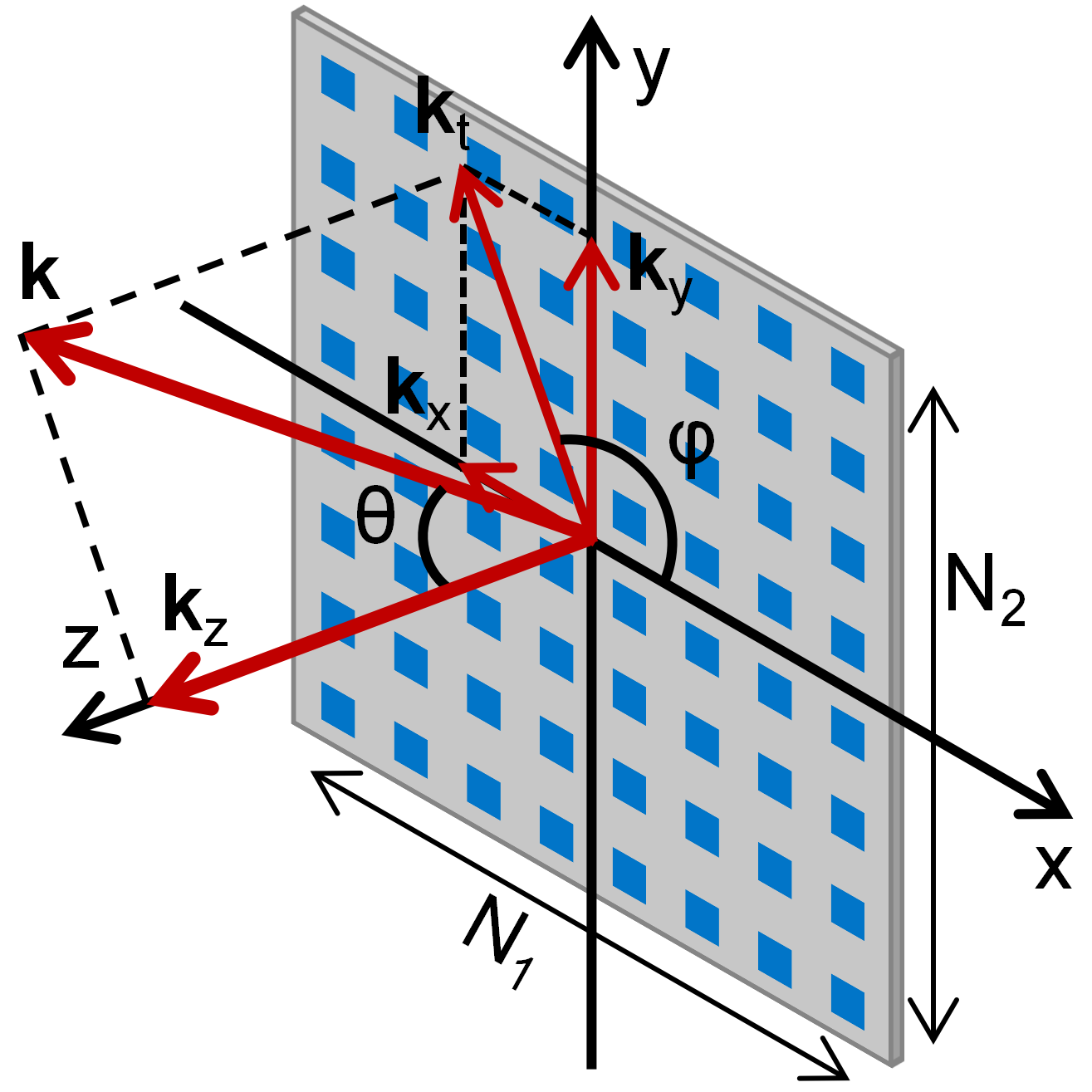
Figure 1: The wave vector $\boldsymbol{k}$ of a transmitted beam in the reference Cartesian and spherical coordinate systems.

In classic electromagnetic theory, there exists a special class of solutions to the Maxwell’s equations in which $k_{x}^{2}+k_{y}^{2}>k^{2}$[14]. If the dispersion relation (3) is to hold true, $k_{z}$ should become an imaginary wavenumber, which leads to an exponential decay to the wave amplitude when it propagate towards z direction. Such solutions are referred to as the evanescent waves and a typical case that an evanescent wave occurs is the total internal reflection on a glass-air interface[16]. Due to the exponential decay, the wave cannot propagate effectively in z-direction.

On the other hand, the wave can still propagate in the x-o-y plane, but with a higher transverse wavenumber $k_{t}=(k_{x}^{2}+k_{y}^{2})^{\frac{1}{2}}$. An evanescent wave belongs to a non-propagation mode, typically arising on sub-wave-length structures or interfaces where discontinuity or inhomogeneity exists[18, 17, 19]. Hence, the evanescent wave usually remains confined near an interface (“reactive boundary” in [18]) and the propagation along the interface exhibits primarily oscillatory behavior. Since the evanescent wave has a higher transverse wavenumber, it possesses a shorter wavelength than a plane wave with the same temporal frequency and propagates slower along the surface in which it is guided. There are also complicated transition mechanisms between the evanescent wave and the propagating wave [20, 17] on sub-wavelength structures. In general, an evanescent wave component is not able to propagate to far field, rendering it impractical for long distance communications. We will see in Section III that an evanescent codeword represent an evanescent component, which is why we have named it as such.

II-B The Far-field Channel Model

The propagation of a plane wave can be regarded as a match between the propagation mode and the wireless channel. The propagation mode of a plane wave is characterized by the phase gradient of the wave on the array plane as it determines the beam direction. As shown in Fig. 1, for a UPA with $N_{1}$ antennas in the x-direction and $N_{2}$ antennas in the y-direction, the lossless line-of-sight (LOS) channel between the antenna located at the $n_{1}$-th row and $n_{2}$-th column of the array and the receiving antenna in the $(\theta,\varphi)$ direction can be expressed as

$$h_{n_{1}n_{2}}(\theta,\varphi)=e^{-j\left(k_{x}n_{1}d_{1}+k_{y}n_{2}d_{2}\right)},$$ (4)

where

$$k_{x}=k\sin\theta\cos\varphi,\quad k_{y}=k\sin\theta\sin\varphi,$$ (5)

and $n_{1}\in\{0,1,\cdots,N_{1}-1\}$, $n_{2}\in\{0,1,\cdots,N_{2}-1\}$. The antenna spacing in the $x$ and $y$ directions are denoted by $d_{1}$ and $d_{2}$, respectively.

Remark 2. By comparing equation (4) to (2), we find that the propagation of an electromagnetic wave is determined by the wavenumber $k_{x}$, $k_{y}$ and $k_{z}$, yet the channel for propagating this electromagnetic wave specifies only $k_{x}$ and $k_{y}$. Although $k_{z}$ is not explicitly expressed in the channel model, it is determined by $k_{x}$ and $k_{y}$ via the dispersion relation (3). For any propagation mode, $k_{x}$, $k_{y}$ and $k_{z}$ should be real number and the transverse wavenumber projected on an array plane $k_{t}=(k_{x}^{2}+k_{y}^{2})^{\frac{1}{2}}$ will not exceed $k$. That is, the LOS wireless channel is a low-pass spatial filter with passband, which has been addressed in [11] and many other studies.

The actual wireless channel is more complex than the single-path LOS channel. For instance, the non-line-of-sight (NLOS) channel in 3GPP TR 38.901 [21] is modeled as clusters comprising multiple rays within a specific angular range. Nonetheless, each ray in the NLOS model can still be represented using the far-field LOS model (4). Consequently, from the perspective of the transmitting array, the NLOS channel is essentially a superposition of several pseudo-LOS channels.

II-C The Kronecker-product Based Codewords

For the UPA shown in Fig. 1, the precoding for directing a beam in a particular direction can be achieved using the Kronecker product of two steering vectors that represent the phase gradients $k_{x}$ and $k_{y}$, respectively. In the standards for 4G and 5G communications, the one-dimensional orthogonal DFT bases are utilized as the steering vectors and the Kronecker-product based codeword can be expressed as [10]

$$\boldsymbol{v}_{lm}= \left\{\left[1,e^{j\frac{2\pi l}{N_{1}O_{1}}},\cdots,e^{j(N_{1}-1)\frac{2\pi l}{N_{1}O_{1}}}\right]\right.\otimes$$ (6)

$$\;\;\left.\left[1,e^{j\frac{2\pi m}{N_{2}O_{1}}},\cdots,e^{j(N_{2}-1)\frac{2\pi l}{N_{2}O_{2}}}\right]\right\}^{T},$$

where $l\in\{0,1,\cdots,N_{1}O_{1}-1\}$, $m\in\{0,1,\cdots,N_{2}O_{2}-1\}$, with $O_{1}$ and $O_{2}$ indicating the oversampling factors. There are $N_{1}O_{1}$ and $N_{2}O_{2}$ DFT bases in the horizontal and vertical directions respectively and the Kronecker-product based codebook comprise a total of $N_{1}O_{1}*N_{2}O_{2}$ codewords.

The codeword $\boldsymbol{v}_{lm}$ has constant phase gradients in two orthogonal directions,

$$k_{1}=\frac{2\pi l}{N_{1}O_{1}},\quad k_{2}=\frac{2\pi m}{N_{2}O_{2}}.$$ (7)

The phase gradients $k_{1}$ and $k_{2}$ represent the spatial frequencies of the codeword in two orthogonal directions. We need to emphasize that $k_{1}$ and $k_{2}$ are in fact the nominal phase gradients. The actual phase gradient of the codeword depends on the antenna spacing of the array on which the codeword is applied. A same codeword will exhibit a different spatial phase gradient on arrays with varying antenna spacing, hence generating beams at different direction. When considering dual-polarization signals, multi-layer transmissions and multi-user MIMO cases, the Kronecker-product codewords are utilized as bases for composing codewords of type-I, type-II or enhanced Type-II. Hence, the Kronecker-product based codewords defined by (6) are also known as the spatial domain bases. In this paper, we will focus on the Kronecker-product based codewords, hence the codebooks and codewords mentioned in subsequent sections refer to the Kronecker-product based ones. For simplicity, a kronecker-product based codebook will be denoted as $\mathbf{CB}_{N_{1},N_{2}}^{O_{1},O_{2}}$. For instance, $\mathbf{CB}_{8,8}^{4,4}$ represents a codebook with $N_{1}=N_{2}=8$ and $O_{1}=O_{2}=4$.

III The Evanescent Codewords

While the Kronecker product allows for a structured indexing for codewords in the codebooks, it also introduces redundant codeword. This redundancy is due to an overlook of a physical constraint in the Kronecker product operation and it will be analyzed in both mathematical and electromagnetic aspects in this section.

III-A The Mathematical Aspect

Theoretically, the codeword $\boldsymbol{v}_{lm}$ represents a spatial beam that matches a particular LOS channel, i.e., $v_{lm,n_{1}n_{2}}=h_{n_{1}n_{2}}^{*}(\theta,\varphi)$, which yields

$$e^{j2\pi\left(\frac{n_{1}l}{N_{1}O_{1}}+\frac{n_{2}m}{N_{2}O_{2}}\right)}=e^{j(n_{1}k_{x}d_{1}+n_{2}k_{y}d_{2})}.$$ (8)

Since $k_{x}=k\sin\theta\cos\varphi$ and $k_{y}=k\sin\theta\sin\varphi$, the angle $(\theta,\varphi)$ of the beam corresponding to $\boldsymbol{v}_{lm}$ can be obtained by solving the above equation. To simplify the analysis, we first rewrite (8) as

$$e^{j2\pi\left(\frac{n_{1}l^{\prime}}{N_{1}O_{1}}+\frac{n_{2}m^{\prime}}{N_{2}O_{2}}\right)}=e^{j(n_{1}k_{x}d_{1}+n_{2}k_{y}d_{2})},$$ (9)

where

$$l^{\prime}=\left\{\begin{aligned} &l,&&l\leq N_{1}O_{1}/2,\\ &l-N_{1}O_{1},&&\text{otherwise},\end{aligned}\right.$$ (10)

$$\quad m^{\prime}=\left\{\begin{aligned} &m,&&m\leq N_{2}O_{2}/2,\\ &m-N_{2}O_{2},&&\text{otherwise}.\end{aligned}\right.$$ (11)

In equation (9), we have replaced the index $(l,m)$ with $(l^{\prime},m^{\prime})$, leveraging the identity $e^{ja}=e^{j(a+2n\pi)}$ where $a\in\mathbb{R}$ and $n\in\mathbb{Z}$. This substitution shifts the ranges of the nominal phase gradient $k_{1}$ and $k_{2}$ in (7) from $[0,2\pi)$ to $(-\pi,\pi]$. According to (9), we obtain

$$2\pi(n_{1}\alpha_{1}\sin\theta\cos\varphi+n_{2}\alpha_{2}\sin\theta\sin\varphi)$$ (12)

$$=2\pi\left(\frac{n_{1}l^{\prime}}{N_{1}O_{1}}+\frac{n_{2}m^{\prime}}{N_{2}O_{2}}\right)+2A\pi,\;A\in\mathbb{Z},$$

where $\alpha_{1}=\frac{d_{1}}{\lambda}$ and $\alpha_{2}=\frac{d_{2}}{\lambda}$ are the normalized antenna spacing. Equation (12) should hold for UPAs with different number of antennas, i.e. $n_{1}$ and $n_{2}$ can be any integers, hence it can be decoupled into the following two equations,

$$\sin\theta\cos\varphi=\frac{1}{\alpha_{1}}\left(\frac{l^{\prime}}{N_{1}O_{1}}+A_{1}\right),$$ (13)

$$\sin\theta\sin\varphi=\frac{1}{\alpha_{2}}\left(\frac{m^{\prime}}{N_{2}O_{2}}+A_{2}\right),$$ (14)

where $A_{1},A_{2}\in\mathbb{Z}$. The beam direction $(\theta,\varphi)$ corresponds to each codeword defined in (6) can now be obtained by solving (13) and (14).

Proposition 1. A codeword $\boldsymbol{v}_{lm}$ defined by (6) is incapable of generating a directional beam on a UPA if its index $(l,m)$ does not satisfy the following inequality,

$$\left(\frac{l^{\prime}}{\alpha_{1}N_{1}O_{1}}\right)^{2}+\left(\frac{m^{\prime}}{\alpha_{2}N_{2}O_{2}}\right)^{2}\leq 1,$$ (15)

where $(l,m)$ relates to $(l^{\prime},m^{\prime})$ by equations (10) and (11).

Proof:

Squaring both sides of equations (13) and (14) and summing the results yields

$$\sin^{2}\theta=\frac{1}{\alpha_{1}^{2}}\left(\frac{l^{\prime}}{N_{1}O_{1}}+A_{1}\right)^{2}+\frac{1}{\alpha_{2}^{2}}\left(\frac{m^{\prime}}{N_{2}O_{2}}+A_{2}\right)^{2}.$$ (16)

Given that $\sin^{2}\theta$ is restricted to the range $[0,1]$ for any real elevation angle, it necessitates the following inequality,

$$\frac{1}{\alpha_{1}^{2}}\left(\frac{l^{\prime}}{N_{1}O_{1}}+A_{1}\right)^{2}+\frac{1}{\alpha_{2}^{2}}\left(\frac{m^{\prime}}{N_{2}O_{2}}+A_{2}\right)^{2}\leq 1.$$ (17)

To ensure this inequality is satisfied, $A_{1}$ and $A_{2}$ should be selected carefully to minimize $|\frac{l^{\prime}}{N_{1}O_{1}}+A_{1}|$ and $|\frac{m^{\prime}}{N_{2}O_{2}}+A_{2}|$. Since $\frac{l^{\prime}}{N_{1}O_{1}}$ and $\frac{m^{\prime}}{N_{2}O_{2}}$ are both confined in the range $(-0.5,0.5]$, it follows that $|\frac{l^{\prime}}{N_{1}O_{1}}+A_{1}|\geq|\frac{l^{\prime}}{N_{1}O_{1}}|$ and $|\frac{m^{\prime}}{N_{2}O_{2}}+A_{2}|\geq|\frac{m^{\prime}}{N_{2}O_{2}}|$ for $A_{1},A_{2}\in\mathbb{Z}$. Hence, $A_{1}$ and $A_{2}$ should be zero and the inequality (17) is simplified into (15). If $\boldsymbol{v}_{lm}$ does not satisfy the inequality (15), it leads to a beam direction with a complex elevation angle according to (16), which proves that the codeword generate a beam in a non-physical space. ∎

Inequality (15) can also be elucidated from a geometric perspective. Since $l\in\{0,1,\cdots,N_{1}O_{1}-1\}$ and $m\in\{0,1,\cdots,N_{2}O_{2}-1\}$, the coordinate $(\frac{l^{\prime}}{N_{1}O_{1}},\frac{m^{\prime}}{N_{2}O_{2}})$ is confined in a square defined by (-0.5,0.5]$\times$(-0.5,0.5], as illustrated in Fig. 2. In contrast, inequality (15) delineates an ellipse with semi-major axis $\alpha_{1}$ and semi-minor axis $\alpha_{2}$. To satisfy (15), $(\frac{l^{\prime}}{N_{1}O_{1}},\frac{m^{\prime}}{N_{2}O_{2}})$ should reside within the intersection of the square and the ellipse. If $A_{1}$ or $A_{2}$ is non-zero, the square will shift away from the ellipse, resulting in less or no overlapping.

In this paper, $\boldsymbol{v}_{lm}$ is termed an evanescent codeword if its index violates (15); otherwise, it is considered as a regular codeword. Evanescent codewords are deemed redundant for far-field transmission due to their inability to generate directional beams, which will be verified in Section IV. Additionally, these codewords are generally superfluous for near-field transmission in the Fresnel zone, a topic that will further discussed in Section V.

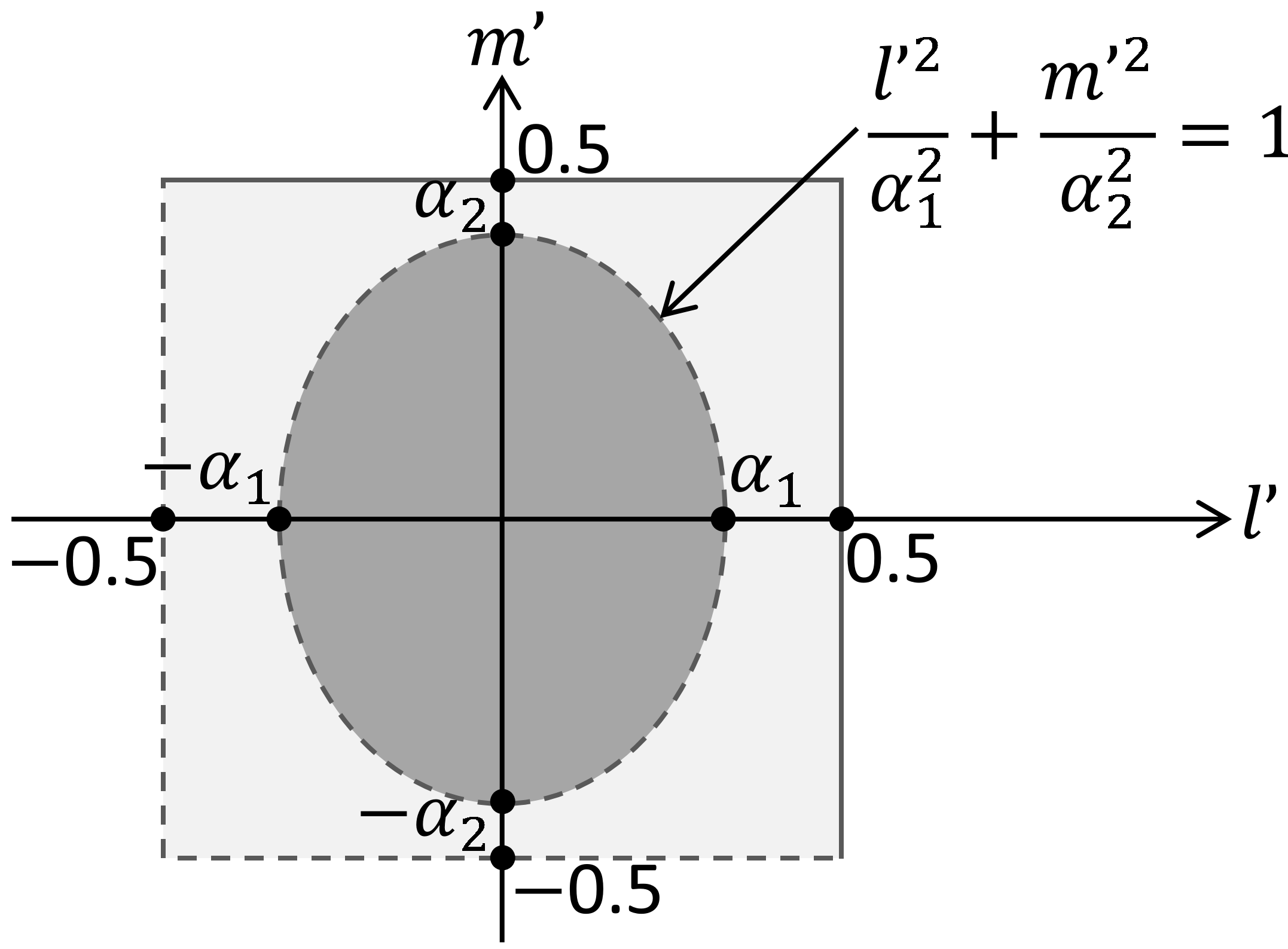
Figure 2: Illustration of the square confined by the indices of the codewords and the ellipse confined by inequality (15).

Based on equations (13) and (14), we further obtain the azimuth of a beam corresponding to $\boldsymbol{v}_{lm}$ as following

$$\varphi=\arctan\left(\frac{m^{\prime}}{l^{\prime}}\frac{\alpha_{1}N_{1}O_{1}}{\alpha_{2}N_{2}O_{2}}\right).$$ (18)

There is no doubt that the azimuth will always be real for any codeword in a Kronecker-product based codebook. The azimuth indicates the direction of the transverse wave vector $\boldsymbol{k}_{t}$ of the wave component represented by a codeword. Fig. 3 shows the distribution of the evanescent codewords in $\mathbf{CB}_{8,8}^{4,4}$ for $\alpha_{1}=\alpha_{2}=0.5$ in the index space. Interestingly, the two sub-figures indicates that the replacement of $(l,m)$ by $(l^{\prime},m^{\prime})$ is in fact a DFT-shift that relocate the zero-frequency component to the center. Clearly, the evanescent codewords gather in a specific region in the index space, termed the evanescent zone, while outsize this region is the regular zone. Fig. 3b is indeed a pixelated version of Fig. 2 for $\alpha_{1}=\alpha_{2}=0.5$ and the jagged boundary between the evanescent and regular zones will approach a perfect ellipse when $O_{1},O_{2}\to\infty$.

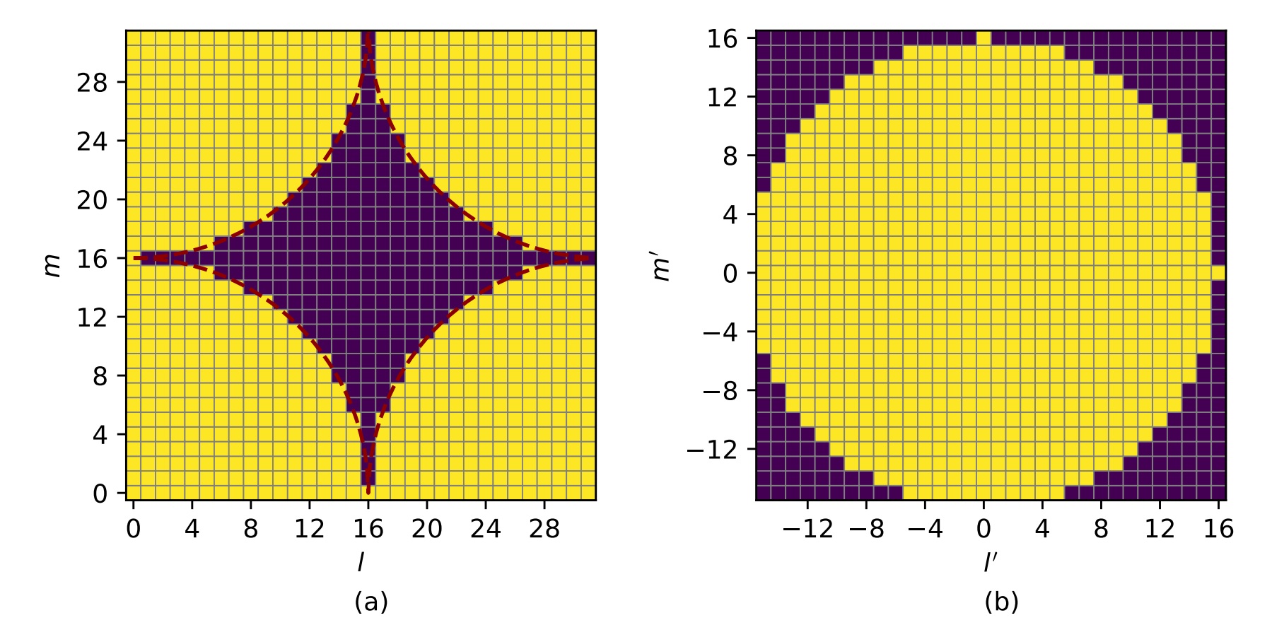
Figure 3: The distribution of regular and evanescent codewords in the index space for $N_{1}=N_{2}=8$, $O_{1}=O_{2}=4$ and $\alpha_{1}=\alpha_{2}=0.5$. The dark purple patches indicate the evanescent codewords. The dashed curves indicate the boundary defined by (15).

Remark 3. The number of evanescent codewords in a Kronecker-product based codebook applied on an array varies with the normalized antenna spacing $\alpha_{1}$ and $\alpha_{2}$. As illustrated in Fig. 2, the ratio of the number of evanescent codewords to the total number of all codewords is quantified as $(1-A_{o}/A_{s})$ when $O_{1},O_{2}\to\infty$, where $A_{o}$ represents the area of the overlapping region between the square and ellipse while $A_{s}$ denotes the area of the square. The area $A_{o}$ varies with $\alpha_{1}$ and $\alpha_{2}$. Notably, this ratio becomes $(1-\pi/4)$ when $\alpha_{1}=\alpha_{2}=0.5$, resulting in a redundancy of about 21.5%. It is evident that the ratio diminishes as $\alpha_{1}$ and $\alpha_{2}$ increase. Hence, whether a codeword is evanescent or regular depends on the antenna spacing of the array to which it is applied. When $\alpha_{1}=\alpha_{2}\geq\frac{\sqrt{2}}{2}$, there is no evanescent codeword in Kronecker-product bases codebooks, regardless of $N_{1}$, $N_{2}$, $O_{1}$ and $O_{2}$ configurations.

III-B The Electromagnetic Aspect

According to (9), we observe that a codeword corresponds to a wave propagation characterized by a transverse wave vector $\boldsymbol{k}_{t}=(k_{x},k_{y})$. Specifically, the index of a codeword relates to $k_{x}$ and $k_{y}$ by $k_{x}=\frac{2\pi}{d_{1}}\frac{l^{\prime}}{N_{1}O_{1}}$ and $k_{y}=\frac{2\pi}{d_{2}}\frac{m^{\prime}}{N_{2}O_{2}}$. Given that $k=\frac{2\pi}{\lambda}$, $\alpha_{1}=\frac{d_{1}}{\lambda}$ and $\alpha_{2}=\frac{d_{2}}{\lambda}$, it follows that

$$k_{x}=\frac{l^{\prime}}{\alpha_{1}N_{1}O_{1}}k,\quad k_{y}=\frac{m^{\prime}}{\alpha_{2}N_{2}O_{2}}k.$$ (19)

Substituting the above equations into (15) yields an equivalent condition for identifying an evanescent codeword based on its spatial frequency,

$$k_{x}^{2}+k_{y}^{2}\leq k^{2}.$$ (20)

We can infer from (20) that, if the index of a codeword fails to meet (15), the resultant wave component has a transverse wavenumber that surpasses $k$. As it is demonstrated in Section II, the violation of (20) leads to an evanescent wave. This is where the name “evanescent codeword” comes from. Clearly, the evanescent zone represent wave components with higher spatial frequencies than $k$.

IV Simulation results

It is proved that the Kronecker-product based codebooks contain evanescent codewords that represent non-propagating wave components rather than directional beams in the previous section. The beam patterns of regular and evanescent codewords will be compared by employing both array synthesis theory and full waveform simulations to verify the redundancy of evanescent codwords in this section. We will further examine the impact of the removal of the evanescent codewords to the throughput performance in system-level simulations.

IV-A Beam Pattern Analysis

To analyze the spatial beam patterns of the codewords, an beamforming model similar to the one for reconfigurable intelligent surface (RIS) in our previous study [22, Eqs. (6) and (7)] is adopted. In contrast to the reflection from a RIS, the array beamforming model does not involve the reflection coefficient and the incident phase delays. Assume that an array is equipped with $N$ antennas, where the $i$-th antenna locates at $\mathbf{r}_{i}$, $i\in{1,2,\cdots,N}$ and a single-antenna UE receives the transmitted signal at $\mathbf{r}^{\prime}$, then the received power can be expressed as

$$P(\mathbf{r}^{\prime})=S\left|\sum_{i=1}^{N}\frac{\sqrt{P_{i}F_{n}(\theta_{i},\varphi_{i})}}{|\mathbf{\mathbf{r}_{i}-\mathbf{r}^{\prime}}|}e^{-jk|\mathbf{\mathbf{r}_{i}-\mathbf{r}^{\prime}}|}\boldsymbol{v}_{l,m}\right|^{2},$$ (21)

where $P_{i}$ and $F_{n}(\theta_{i},\varphi_{i})$ denote the transmission power and power-normalized radiation pattern of the $i$-th antenna, respectively, $(\theta_{i},\varphi_{i})$ being the angles of departure with respect to the $i$-th antenna. The effective aperture of the UE antenna $S$ is presumed to be the actual area of the antenna (e.g., $S=\lambda^{2}/4$). To simplify the analysis, isotropic radiation pattern is assumed for the transmission antenna, i.e. $F_{n}=\frac{1}{2\pi}$.

In order to visualize the beam pattern of a specific codeword, we calculated the received power on a hemispherical surface at the far-field region, as demonstrated in Fig.1b in [22]. Fig. 4a and Fig. 4b show respectively the beam patterns of the regular codeword $\boldsymbol{v}_{4,10}$ and the evanescent codeword $\boldsymbol{v}_{14,16}$ from $\mathbf{CB}_{8,8}^{4,4}$. A directional beam towards $\theta=42.3^{\circ}$ and $\varphi=68.2^{\circ}$ was generated by $\boldsymbol{v}_{4,10}$ while no distinguishable main lobe appeared in the beam pattern of $\boldsymbol{v}_{14,16}$. When $\boldsymbol{v}_{14,16}$ was applied, the energy primarily radiated along the edge of the array while no significant radiation was observed in the normal direction, consistent with the aforementioned characteristics of evanescent waves.

In regard to an actual antenna array with dedicated design for the antenna units, complex mutual coupling exist among antennas [23] and the beam pattern may be reshaped. Furthermore, there are transitions between evanescent mode and propagation mode via sub-wavelength structures in the array. The beamforming simulation via array synthesis with ideal point source assumption falls short of capturing the coupling and transition. Conversely, full waveform methods, such as discontinuous Galerkin methods [24], which takes into account the interaction between the radiated electromagnetic field and the array structure, obtain the electromagnetic field distribution by solving a boundary value problem involving Maxwell’s equations and specific boundary conditions. Hence, full waveform simulations were conducted to further confirm the beam pattern of evanescent codewords.

A dual-polarized antenna array with product-level design, operating at the 6.7 GHz band, was employed for the simulation. The array was equipped with 8 rows and 8 columns of antennas, each with size of half-wavelength ($\approx$ 22.4 *22.4 mm²). As depicted in Fig. 4c and 4d, the beam patterns are similar to the results from the array synthesis, which indicates that the mutual coupling does not significantly affect the beam pattern in this array. Both array synthesis and full waveform simulation demonstrate that the evanescent codewords cannot generate directional beam in physical space, deeming them redundant in far-field transmission. The simulation results also indicate that, when the antenna spacing is not sufficient small, array synthesis based simulation is accurate enough for beam pattern analysis. According to the full waveform simulations, even though the array can still radiate energy with evanescent codewords, the maximum radiation power under the precoding $\boldsymbol{v}_{14,16}$ is about 10.5 dB lower than that of $\boldsymbol{v}_{4,10}$. Additionally, stronger radiation in the normal direction is witnessed in full waveform simulation, which may indicate a small portion of the evanescent component is transformed into propagating mode.

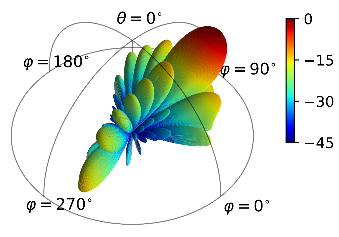
(a)

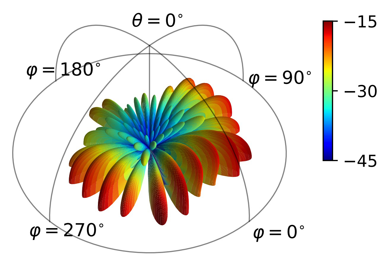
(b)

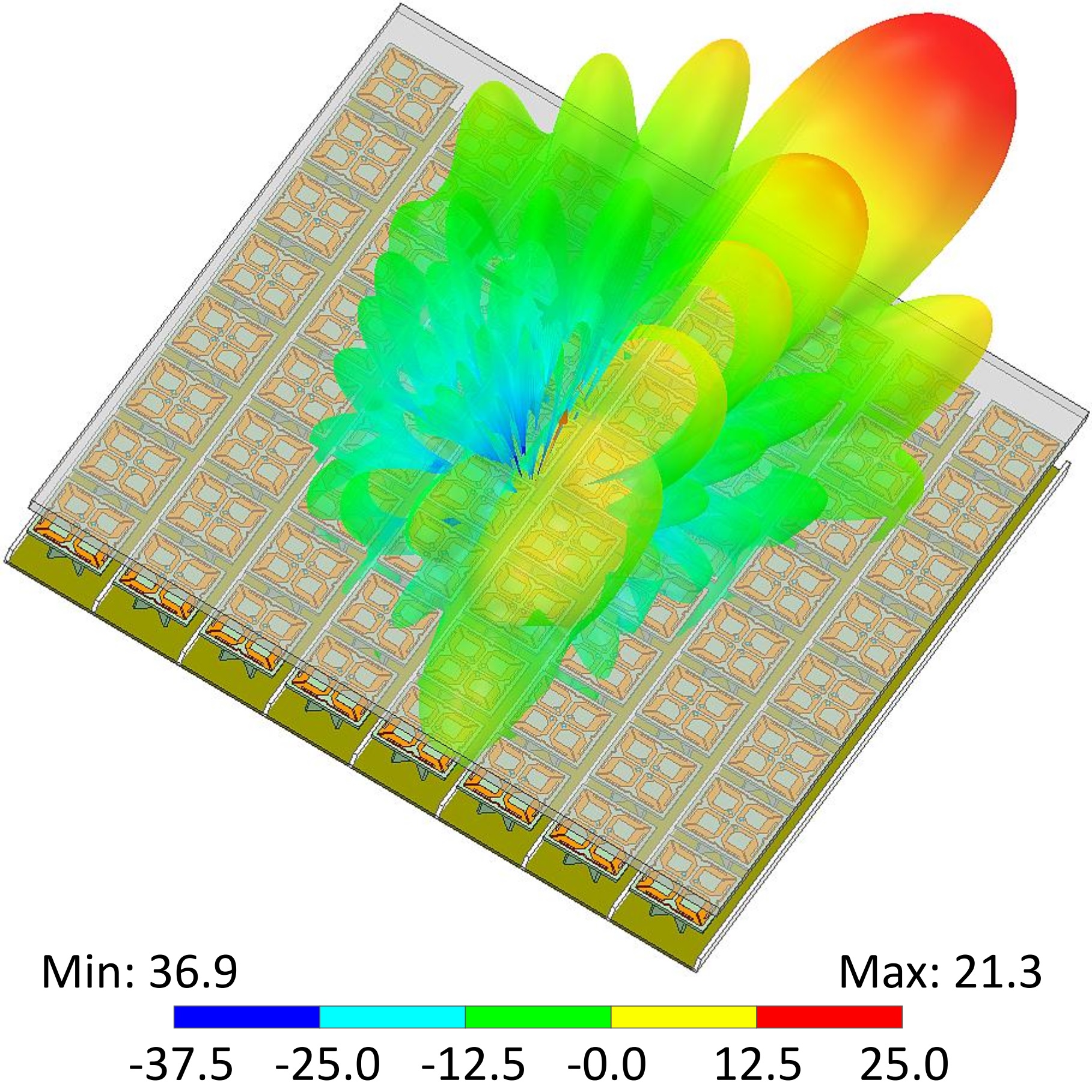
(c)

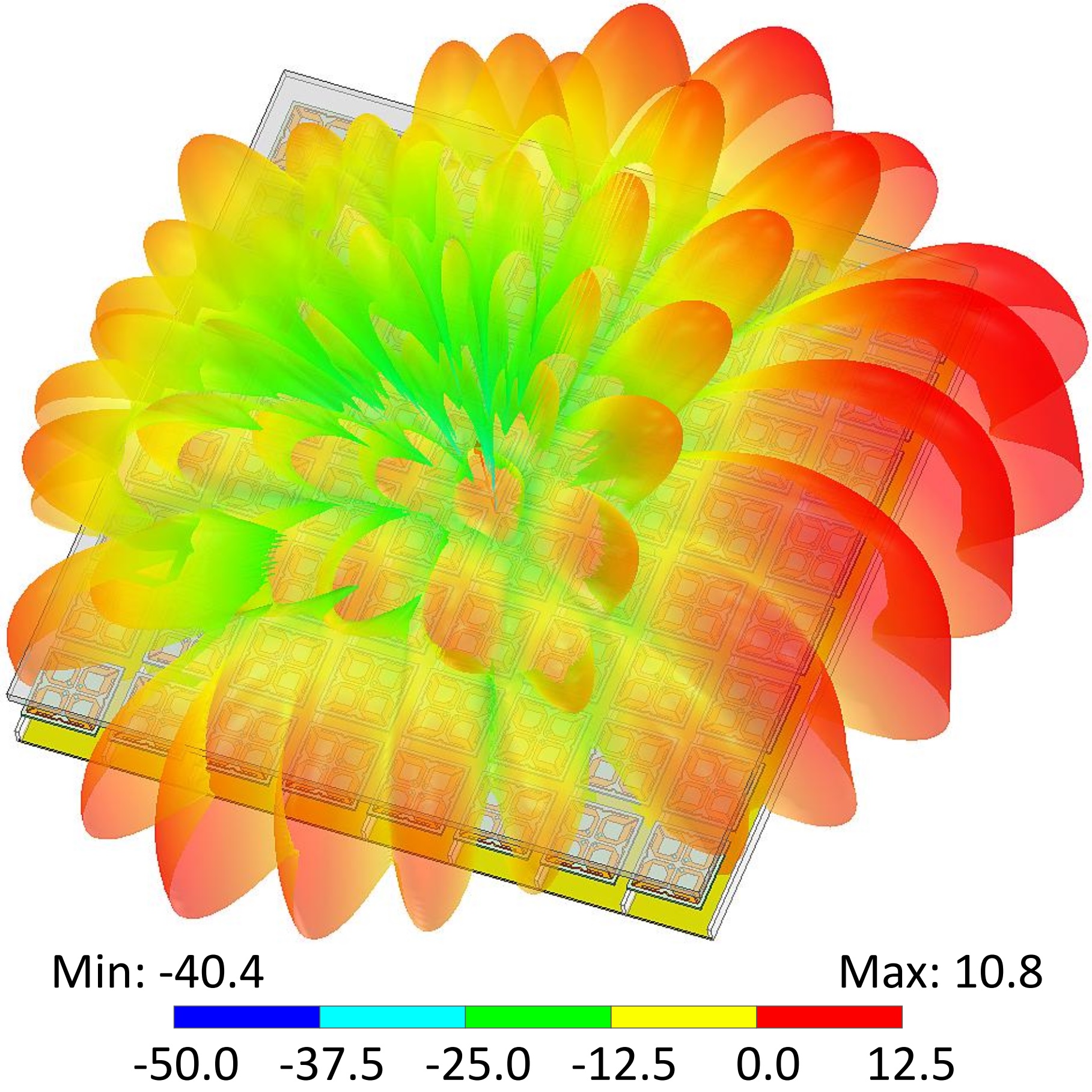
(d)

Figure 4: Beam patterns of codewords $\boldsymbol{v}_{4,10}$ (left column) and $\boldsymbol{v}_{14,16}$ (right column) from $\mathbf{CB}_{8,8}^{4,4}$. Subplots (a) and (b) are based on antenna synthesis theory while (c) and (d) are based on full waveform simulation.

IV-B System Level Simulations

Since evanescent codeowrds do not align with any physical channel, the exclusion of the codewords in the evanescent zone should not impact the system throughput performance in MIMO communications. To substantiate this presumption, a system level simulation with codebook subset restriction (CBSR) [10] was conducted in our NR simulation platform. The 3GPP indoor-office scenario, as depicted in Fig.7.2-1 and Table 7.2-2 in [21], was adopted for the simulation. Twelve base stations (i.e., gNB), each equipped with 8$\times$8 dual-polarized and half-wavelength antennas, were mounted on the office ceiling, 3 m above the ground and 20 m apart. The office (120 m$\times$50 m) was partitioned into 12 sectors and each gNB served one sector that contains 15 uniformly distributed UEs. The UEs, equipped with 2$\times$2 dual-polarized half-wavelength antennas, were moving at a height of 1 m from the ground. The detailed parameters for the simulations are summarized in Table I. To better meet the requirement of real-world transmission, the following setup was also applied in the simulations: (1) a high-precision enhanced Type II codebook based on $\mathbf{CB}_{8,8}^{4,4}$ was utilized for precoding matrix indicator (PMI) reporting; (2) PMIs were reported on a resource block (RB) level, i.e., one PMI report per RB; (3) FTP traffic model 1 [25] was chosen for multi-user transmission; (4) the modulation coding scheme (MCS) and the number of layers for transmission were determined adaptively based on the channel condition.

TABLE I: Setup for system level simulations

Parameter	Value
Carrier Frequency	6 GHz
Channel Model	TR 38.901 indoor-office setup [21]
Antenna setup and port layouts at gNB	(M, N, P, Mg, Ng, Mp, Np) =(8,8,2,1,1,8,8) (dH, dV) = (0.5 $\lambda$, 0.5 $\lambda$)
Antenna setup and port layouts at UE	(M, N, P, Mg, Ng, Mp, Np) =(1,2,2,1,1,1,2) (dH, dV) = (0.5 $\lambda$, 0.5 $\lambda$)
Modulation	Up to 256 QAM
gNB Tx power	44 dBm
UE Tx power	23 dBm
gNB receiver noise figure	5 dB
UE receiver noise figure	9 dB
Numerology	14 OFDM symbol per slot, 15 kHz SCS
UE Bandwidth	10 MHz, 52 RBs
UE reception	MMSE-IRC
UE moving speed	$\leq$ 3 km/h
Network Layout	12 sectors, 15 UEs per sector
CSI feedback delay	5 ms
MIMO scheme	SU/MU-MIMO with rank=1-4 per UE

Firstly, the selection counts of the codewords in $\mathbf{CB}_{8,8}^{4,4}$ were gathered in the indoor simulation without the restriction. As shown in Fig. 5a, the selected codewords were mainly located in the regular zone. Note that, the selection counts exceeding 300 were capped at 300 to better visualize the codewords that were never selected. Theoretically, no evanescent codeword should be selected since they do not beamform efficiently. However, we do observe the selection of evanescent codewords in the vicinity of the boundary between the regular and evanescent zones. There were a total of 253,280 selections with approximately 13.5% being the evanescent codewords. The following three factors should account for the selection of the evanescent codewords.

1. The oversamping factors $O_{1}$ and $O_{2}$: Although the peak of a beam corresponding to an evanescent codeword is not visible in physical space, the side lobes or even a part of the main lobe can still be projected into the physical space due to the limited array aperture. As shown in Fig. 5b, the main lobes generated by the evanescent codewords $\boldsymbol{v}_{13,12}$ and $\boldsymbol{v}_{12,11}$ in $\mathbf{CB}_{8,8}^{4,4}$ remain partially in the physical space. When the UE appears in the light blue zone in Fig. 5c, the evanescent codeword $\boldsymbol{v}_{12,11}$ will be selected instead of $\boldsymbol{v}_{11,10}$ due to its higher power gain in this region. If the oversampling factor of a codebook is sufficient large, we can always find a regular codeword that has better beamforming gain than any evanescent codeword in any physical direction.

2. The interference: When the interference from other cells is strong, the system tends to select other bases rather than the one indicated by the channel measurement according to user scheduling. Furthermore, co-channel interference is usually destructive and results in low SINR, making it more likely to select an inappropriate codeword, including an evanescent codeword.

3. wideband noise: The noise is usually present in a wideband and it appears as a high spatial-frequency component in the received spatial signal. Consequently, when the noise and interference levels are high, which typically presence near the cell border, the system is more prone to mistakenly select an evanescent codeword.

In the indoor simulation, the BSs were mounted on the ceiling and the UEs near the cell border required the serving BS to transmit signals with beams oriented almost horizontally, which correspond to regular codewords near the zone boundary. Consequently, the impacts of the above three factors culminate in the cell border, potentially resulting in the selection of evanescent codewords.

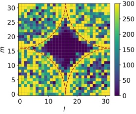
(a)

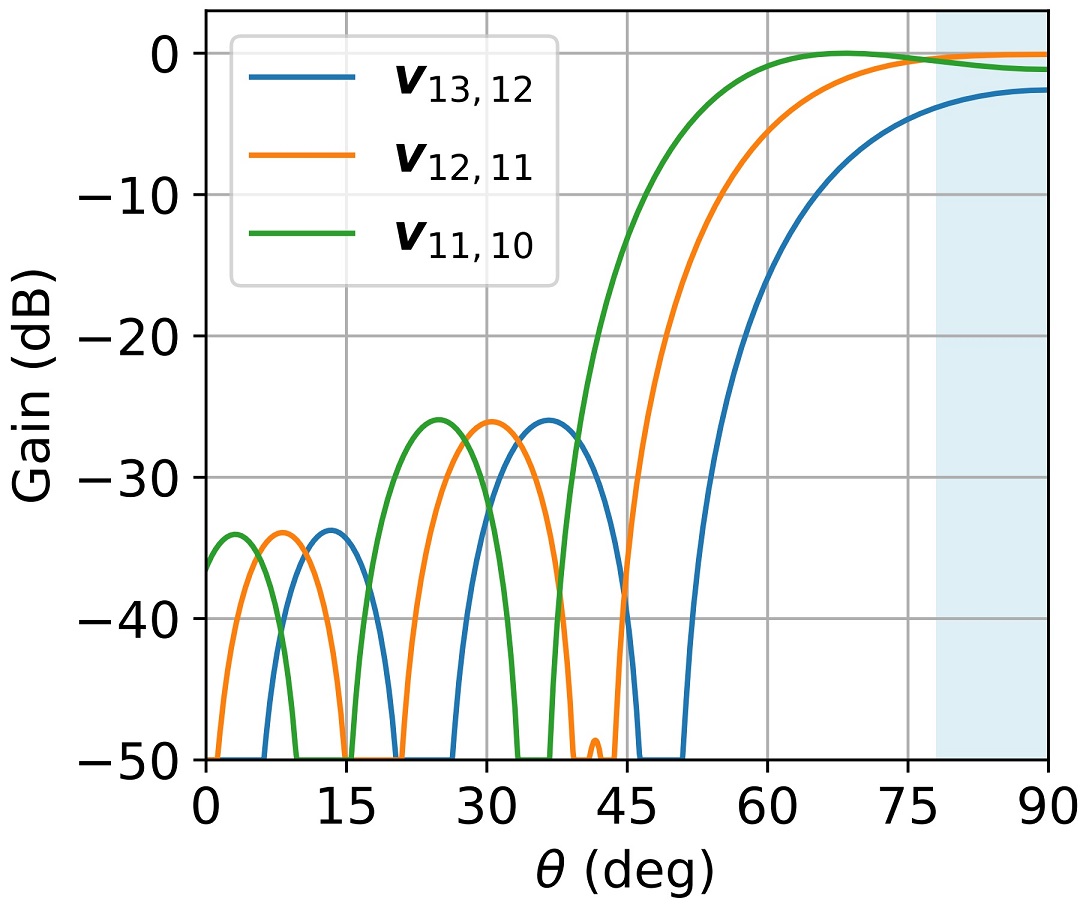
(b)

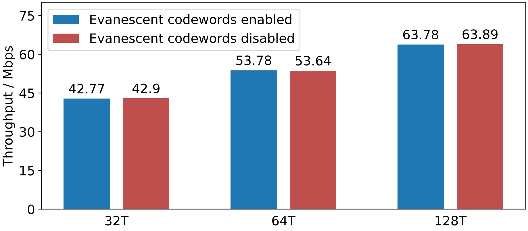
(c)

Figure 5: (a) Heatmap of codeword selection counts in the simulation with 128 ports, (b) beam patterns of $\boldsymbol{v}_{13,12}$, $\boldsymbol{v}_{12,11}$ and $\boldsymbol{v}_{11,10}$ and (c) comparison of the system throughput with and without evanescent codewords enabling. The brown dashed curve in outline the boundary between regular and evanescent zones in index space.

Based on the theoretical channel model without noise and interference, we have proved that the evanescent codewords are redundant in the previous section. However, this theoretical redundancy do not stop the selection of the evanescent codewords in a complex wireless environment. Now we need to verify the redundancy by the throughput performance analysis.

With the CBSR configuration, the selection of evanescent codewords can be enabled or disabled in PMI reporting. Three BS array configurations were chosen for comparison in the simulation, i.e. 32T ($N_{1}=N_{2}=4$, dual-polarized), 64T ($N_{1}=4$, $N_{2}=8$, dual-polarized), 128T ($N_{1}=N_{2}=8$, dual-polarized). As shown in Fig. 5c, the throughputs are almost the same with or without the evanescent codewords in the codeboook. We have stated that the selection of the evanescent codewords mainly caused by interference and noise. In a sense, the disabling of the evanescent codewords may help combat the low SINR condition. However, no significant throughput improvement was shown in the simulations with the evanescent codewords disabled. In fact, the selection of the evanescent codewords was under low SINR. Even if the evanescent codewords were disabled, the throughput would not be significantly improved.

With the beam pattern analysis and system level simulations, we have verified that the evanescent codewords are redundant in MIMO communications. The MIMO system can benefit from disabling these codewords. For one thing, it can reduce the CBSR signaling overhead by about 20% without affecting the system performance. For another, it can speed up the codeword selection and channel report. Additionally, the DFT-based orthogonal beams are usually applied in beam training, hence there are also redundant beams that are not visible in the physical space. Excluding the beams in the evanescent region helps accelerate the beam training due to the reduction in the number of candidate beams.

V Discussions on spatial frequency and spatial sampling

The precoding of a MIMO array can be considered as a spatial sampling of a particular electromagnetic wave and it reconstructs the wave propagation provided that the spatial sampling satisfies the Nyquist criterion, otherwise it gives rise to grating lobes. Although a two-dimensional array samples only a projection of the wave propagation within the array plane, it remains capable of reconstructing the wave propagation since the wave vector is constrained to comply with the dispersion relation (3). For a uniform linear array, the step length for sampling should be smaller than half the wavelength to satisfy the criterion. When it comes to a uniform rectangular sampling grid, the sampling is proceeded in two orthogonal directions and the spatial sampling rate is more complicated. Inspired by the study on spatial sampling in [13], the evanescent codewords will be analyzed from the view point of spatial sampling in this section. Several other related topics will also be involved.

V-A Spatial Sampling for the Evanescent Codewords

Remark 4: The rectangular sampling grid has the highest spatial sampling rate in the diagonal direction and the lowest sampling rate along the orthogonal grid. This remark is quite counter-intuitive at first glance since a larger antenna spacing is presented in the diagonal direction. However, unlike the frequencies in temporal signals, a wave propagating along the sampling plane leads to a vectorized spatial frequency. As shown in Fig. 6a, the wave vector $\mathbf{k}_{t}$ can be decomposed into the two orthogonal components $k_{x}$ and $k_{y}$. As long as the decomposed frequency components do not exceed any of the spatial frequencies $k_{s,x}$ and $k_{s,y}$ supported by the sampling grid, the Nyquist criterion is satisfied.

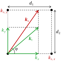
(a)

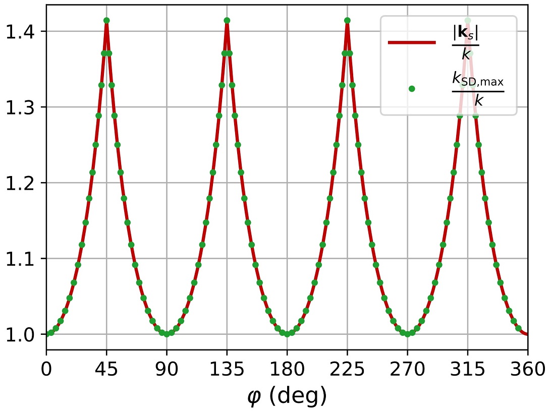
(b)

Figure 6: (a) Illustration of wave vector decomposition in a rectangular grid and (b) maximum spatial frequency supported by a rectangular grid with $\alpha_{1}=\alpha_{2}=0.5$ (solid line) and the maximum spatial frequencies of the evanescent codewords (green dots) at different azimuth.

According to the sampling theorem, the highest spatial frequency supported by a UPA in x- and y-directions can be expressed as

$$k_{s,x}=\frac{2\pi}{2d_{1}}=\frac{k}{2\alpha_{1}},\quad k_{s,y}=\frac{2\pi}{2d_{2}}=\frac{k}{2\alpha_{2}}.$$ (22)

The spatial frequency supported at other direction is determined by the length of $\boldsymbol{k}_{s}$ when its endpoint moves along the squared grid (Fig. 6a). Clearly, the diagonal direction of the grid accommodates the highest spatial frequency while the two orthogonal directions along the grid support the lowest spatial frequency (Fig. 6b, the solid line). Remark 4 can also be explained by the relation between the sampling matrix $\mathbf{Q}$ and the periodicity matrix $\mathbf{P}$ as depicted by Eq. (10) in [13].

TABLE II: Parameters of beams A and B

Precoding No.	$k_{x}$	$k_{y}$	$k_{t}$	Beam direction
$w_{1}$	$k$	0	$k$	$\theta=90^{\circ},\varphi=0^{\circ}$
$w_{2}$	$\frac{\sqrt{2}}{2}k$	$\frac{\sqrt{2}}{2}k$	$k$	$\theta=90^{\circ},\varphi=45^{\circ}$

To examine whether the diagonal direction of the UPA supports a higher spatial frequency or not, we conducted beam pattern simulations for two precodings having the same transverse spatial frequency but pointing at different azimuth, as listed in Table II. The simulations are based on a UPA with $N_{1}=N_{2}=8$ and $\alpha_{1}=\alpha_{2}=0.5$. It is clear that $w_{1}$ is $\boldsymbol{v}_{16,0}$ in $\mathbf{CB}_{8,8}^{4,4}$ but $w_{2}$ does not correspond to any codeword in this codebook and need to be calculated according to (4). As shown in Fig. 7a and 7b, $w_{1}$ generates a beam with a grating lobe at the opposite direction while only the main lobe appears for $w_{2}$, which indicates that a higher spatial frequency is supported in the diagonal direction of a UPA. More specifically, the supported spatial frequency in the diagonal direction is $\sqrt{2}$ times the one along the grid for a UPA with $\alpha_{1}=\alpha_{2}$. As a result, the antenna spacing can be set to be slightly smaller than $\frac{\sqrt{2}}{2}\lambda$ for a UPA to generate a beam towards $\theta=90^{\circ}$ and $\varphi=45^{\circ}$ without grating lobe. We need to emphasize that, the above analysis is valid for wave components propagating along the sampling plane. For wave components with non-zero wavenumber in z-direction, the minimum sampling frequency required is no longer determined only by the transverse spatial frequency and we are not going to involve further discussion in this section.

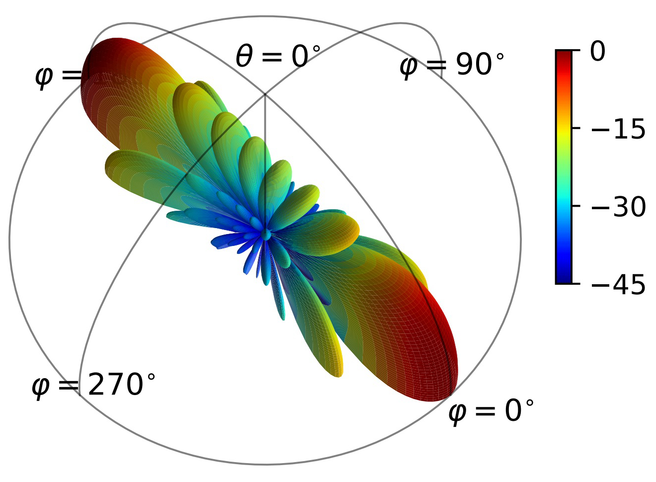
(a)

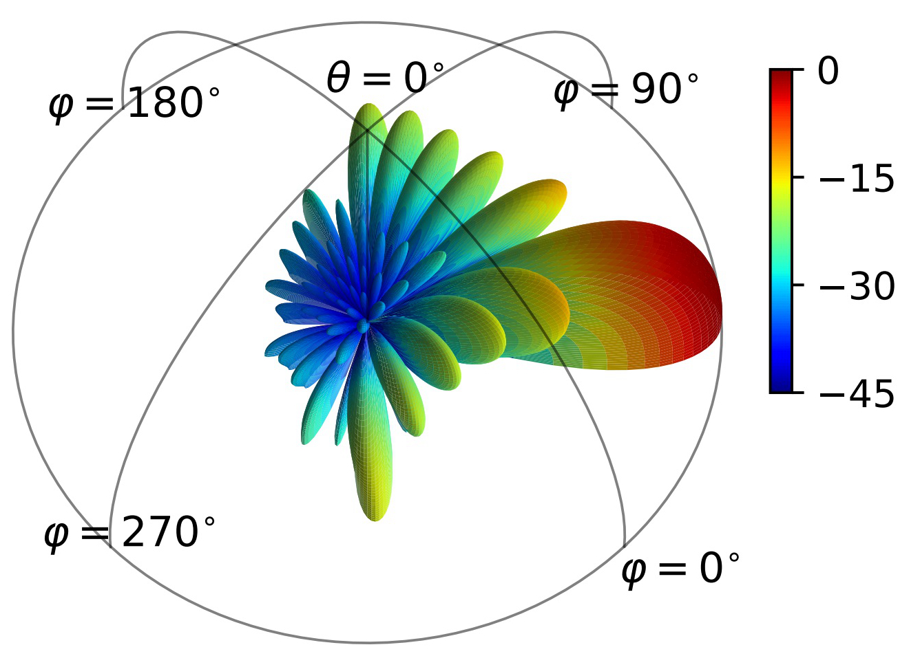
(b)

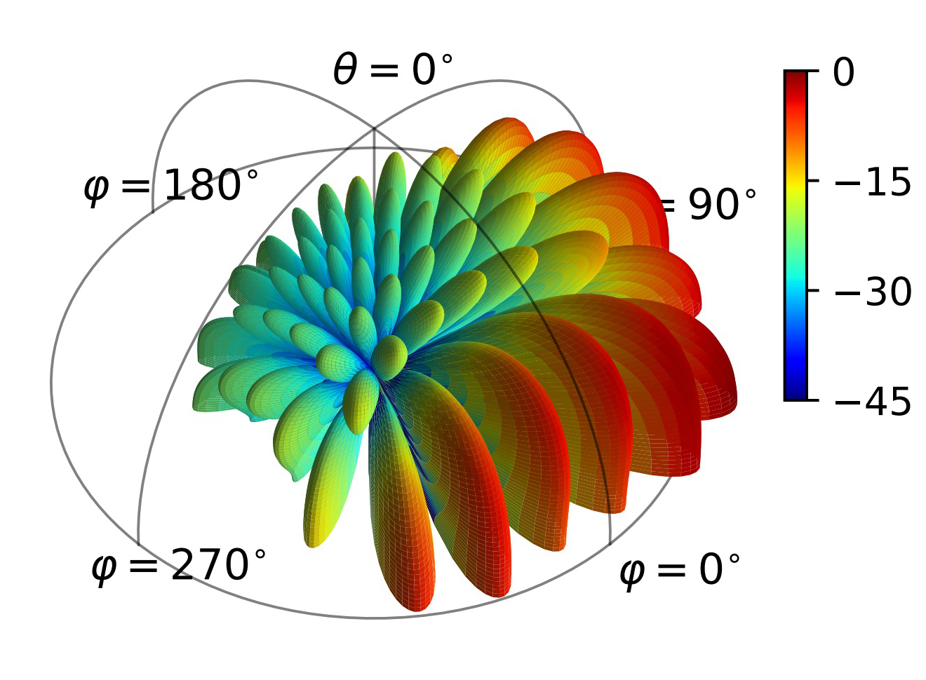
(c)

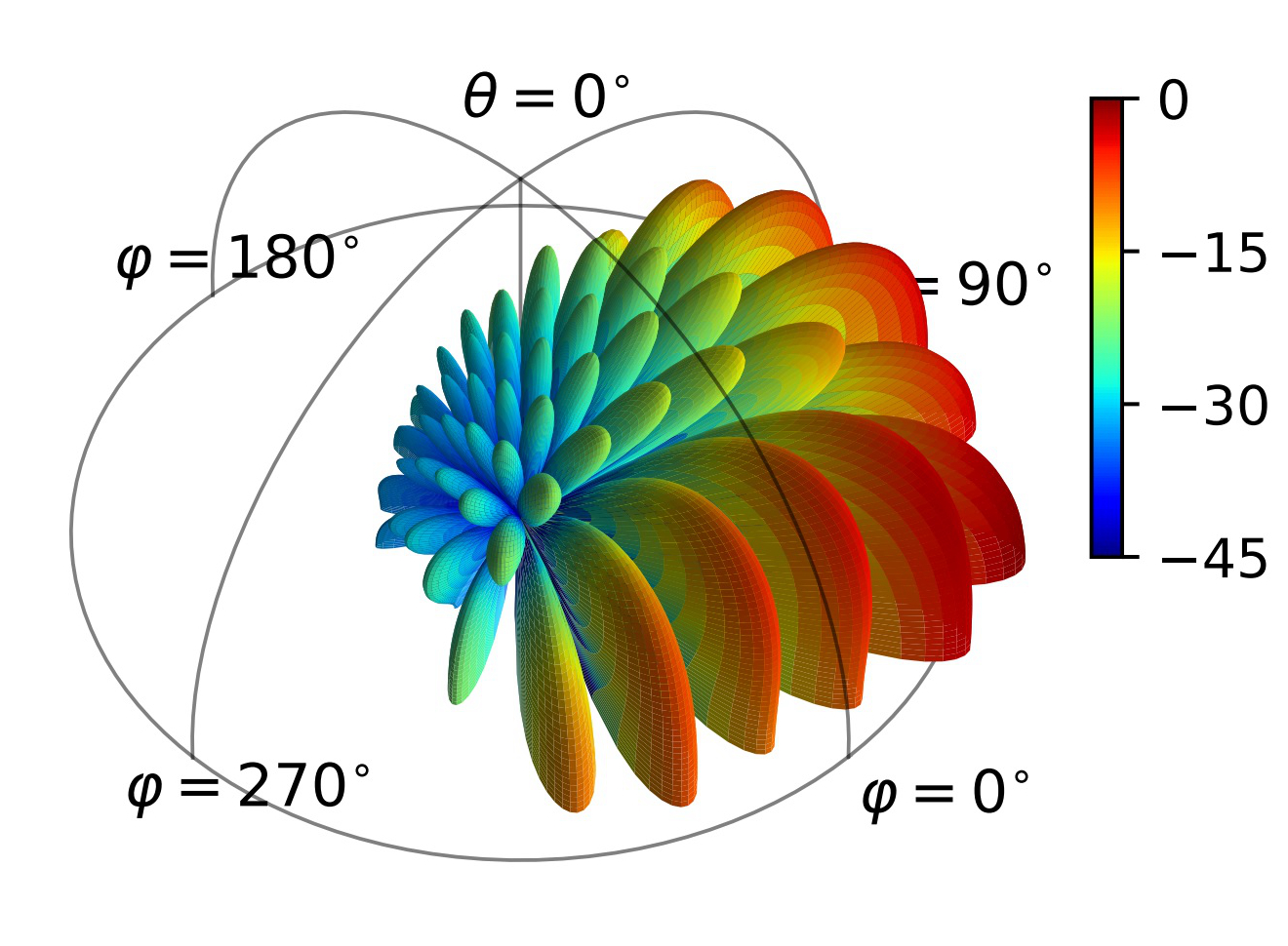
(d)

Figure 7: Beam patterns of precodings (a) $w_{1}$ and (b) $w_{2}$; Beam patterns of precodings with the same phase gradient as the evanescent codeword $\boldsymbol{v}_{14,16}$ on UPAs with (c) $\alpha_{1}=\alpha_{2}=0.4$ and (d) $\alpha_{1}=\alpha_{2}=0.25$.

Since the evanescent codewords represent wave components with spatial frequencies exceeding $k$, the reconstruction of these wave components should require a higher spatial sampling rate. It is necessary to analyze whether the non-directional radiation patterns of the evanescent codewords shown in Figs. 4b and 4d are the result of the spatial undersampling. If so, what is the maximum antenna spacing allowed for the evanescent codewords to generate a beam without grating lobes?

Remark 5: A UPA with antenna spacing slightly smaller than half the wavelength is able to guarantee that the Nyquist sampling criterion be satisfied for all codewords in Kronecker-product based codebooks except the outermost ones in Fig. 3b. The outermost codewords in Fig. 3b are those with index $l=N_{1}O_{1}/2$ or $m=N_{2}O_{2}/2$. According to (19), the codewords $\boldsymbol{v}{N_{1}O_{1}/2,m}$ and $\boldsymbol{v}{l,N_{2}O_{2}/2}$ represent wave components with maximum spatial frequencies of $k_{x,\max}=\frac{k}{2\alpha_{1}}$ and $k_{y,\max}=\frac{k}{2\alpha_{2}}$, respectively, which are exactly the highest spatial frequencies supported by a UPA (see Eq. 21). Note that, there are negative frequencies in spatial domain, the signal should have spatial frequency lower then the highest frequency supported by the UPA to avoid aliasing. Hence, the outermost codewords in Fig. 3b will always generate grating lobes on any UPA regardless of its antenna spacing. Now it is for sure that there are grating lobes in Fig. reff-beam-pat-simb and Fig. reff-beam-pat-simd.

The conclusion in Remark 5 is based on the assumption that the codewords are directly applied on a UPA, which is the common procedure in MIMO system. The direct application of the codewords means that the actual phase gradient of the precoding varies with the antenna spacing, and the highest supported sampling rate of a UPA always dissatisfies the sampling rate required by the outermost codewords. However, if the phase gradient of a selected codeword is considered, we are able to fulfill the sampling criterion for these evanescent codewords by phase interpolation on a UPA. For instance, the basis $\boldsymbol{v}_{14,16}$ that generates beam patterns in Fig. 4b and Fig. 4d has phase gradients $2\pi\frac{14}{32*0.5\lambda}$ in x-direction and $2\pi\frac{16}{32*0.5\lambda}$ in y-direction. By interpolation, we can determine the precoding that has the same phase gradient on a UPA with $d_{1}=d_{2}=0.4\lambda$. Now the wave component can be perfectly reconstructed since the antenna spacing of $0.4\lambda$ meets the sampling criterion. As shown in Fig. 7c, the beam lobes in the azimuth range $180^{\circ},270^{\circ}$ vanishes compared to Fig. reff-beam-pat-simb, indicating the removal of grating lobes. Further diminishing the antenna spacing, e.g., $0.25\lambda$, will slightly lower the side lobe level but will not improve the beamfoeming gain of the main lobe, as shown in Fig. 7d. It is now evident that an evanescent codeword is incapable of generating a directional beam in physical space, even with a dense array.

V-B The Spatial Frequency of the Near-field Channel

There were comprehensive studies on near-field MIMO communications in recent years, as summarized in [26, 27]. It has been found that the near-field channels exhibit lower sparsity in the wave-number domain compared to far-field channels. Hence, a near-field channel contains various spatial-frequency components, but how these components are distributed is yet to be investigated. In this section, we will restrict our discussion to the radiative near-field (Fresnel) region, typically in the range $[0.62\sqrt{\frac{D^{3}}{\lambda}},\frac{2D^{2}}{\lambda})$ [28], where the EM field has negligible radial component and the radiation can be well approximated by spherical wave model.

For a UPA lying in x-o-y plane as shown in Fig. 1, to focus the transmission energy at a UE locating at $(r,\theta,\varphi)$, the phase delay for the antenna locating at (x, y, 0) is determined by the distance between the antenna and the UE, i.e.,

$$\phi(x,y)=kr(x,y),$$ (23)

where the distance $r(x,y)$ is calculated as

$$r(x,y)= \left[(x-r\sin\theta\cos\varphi)^{2}+\right.$$ (24)

$$\left.(y-r\sin\theta\sin\varphi)^{2}+r^{2}\cos^{2}\theta\right]^{\frac{1}{2}}.$$

Proposition 2. The Fresnel near-field channel does not contain evanescent components, i.e., the phase gradient will not exceed $k$.

Proof:

The spatial frequency is determined by the spatial derivatives of the phase distribution, i.e.,

$$k_{x}=\frac{\partial\phi(x,y)}{\partial x}=\frac{k\operatorname{sgn}(x-r\sin\theta\cos\varphi)}{\sqrt{1+\left(\frac{y-r\sin\theta\sin\varphi}{x-r\sin\theta\cos\varphi}\right)^{2}+\left(\frac{r\cos\theta}{x-r\sin\theta\cos\varphi}\right)^{2}}},$$ (25)

and

$$k_{y}=\frac{\partial\phi(x,y)}{\partial y}=\frac{k\operatorname{sgn}(y-r\sin\theta\sin\varphi)}{\sqrt{1+\left(\frac{x-r\sin\theta\cos\varphi}{y-r\sin\theta\sin\varphi}\right)^{2}+\left(\frac{r\cos\theta}{y-r\sin\theta\sin\varphi}\right)^{2}}}.$$ (26)

Since the denominators in (25) and (26) are always greater than or equal to 1, we have $k_{x}\leq k$ and $k_{y}\leq k$. The transverse spatial frequency can then be calculated as following,

$$k_{t}= \sqrt{k_{x}^{2}+k_{y}^{2}}$$ (27)

$$= \frac{k}{\sqrt{1+\frac{r^{2}cos^{2}\theta}{(x-r\sin\theta\cos\varphi)^{2}+(y-r\sin\theta\sin\varphi)^{2}}}}\leq k.$$

Consequently, the Fresnel near-field channel does not contain evanescent components. In other words, a near-field channel only requires the codewords in the regular zone for precoding if the Kronecker-product based codebooks are employed. ∎

To better visualize this proposition, four typical near-field channels are selected to calculate the correlation with the Kronecker-product based codewords. If there are evanescent components in these channels, the energy will be partially projected onto the evanescent codewords. The array is set to be $N_{1}=N_{2}=128$, $\alpha_{1}=\alpha_{2}=0.5$ with the maximum aperture being $D=64\sqrt{2}\lambda$. Four near-field channels corresponding to UE locations $\mathbf{r}_{1}=(D,0^{\circ},0^{\circ})$, $\mathbf{r}_{2}=(D,30^{\circ},45^{\circ})$, $\mathbf{r}_{2}=(D,60^{\circ},45^{\circ})$ and $\mathbf{r}_{2}=(D,90^{\circ},45^{\circ})$ in spherical coordinate system are selected. As shown in Fig. 8, the projected energy spreads out as expected but are confined in the regular zone for different near-field channels. For the lower right sub-figure, the energy lies in the vicinity of the boundary and diffuses slightly into the evanescent zone. This overstepping is due to $O_{1}=O_{2}=1$ in the codebook.

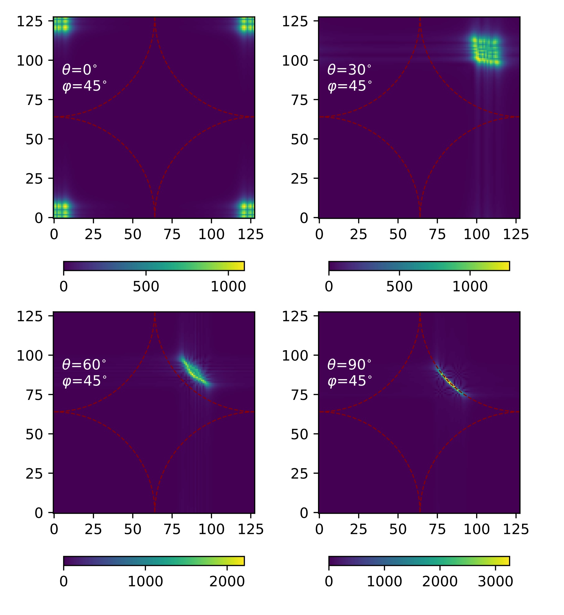
Figure 8: Correlations of four near-field channels with the codewords in $\mathbf{CB}_{128,128}^{1,1}$. The dark red dashed line indicates the boundary between the regular and evanescent zones.

Note that, when $r\to\infty$, we have $k_{x}\approx k\sin\theta\cos\varphi$ and $k_{y}\approx k\sin\theta\sin\varphi$ in (25) and (26). Clearly, the spatial frequency of the near-field channel converges to constants which match the plane wave model at far field, i.e., equation (4). Both far-field and near-field channels act as low-pass spatial filters for signal transmission. However, we need to stress that the spatial frequency of a near-field channel varies with the position of the transmission antenna according to (25) and (26) while a far-field channel exhibits a constant spatial frequency across the array. In other words, non-uniform spatial sampling is allowed for near-field transmission. Nevertheless, a UPA with an antenna spacing that is slightly smaller than half the wavelength is sufficient for any near-field channels, according to Remark 5.

V-C The Rayleigh channel model

The Rayleigh channel model is widely employed for evaluating the performance of various MIMO systems and algorithms due to its straightforward mathematical formulation and favorable statistical properties. However, the Rayleigh channel neglects the low-pass characteristic of physical channels, potentially including evanescent components in randomly generated channels. As discussed in Section III, to enhance realism, we propose modifying the Rayleigh channel model through the following steps: (1) Perform a Discrete Fourier Transform (DFT) on the randomly generated Rayleigh channel; (2) In the transformed domain, zero out the amplitudes of components in the evanescent zone using equation (15); (3) Transform the modified channel back to the spatial domain with inverse DFT. When prior spatial frequency information is available, a more accurate Rayleigh channel model can be established by eliminating spatial frequency components that are absent in the wave-number domain.

V-D The Evanescent Zone in Wideband Communications

The analysis of the evanescent codewords in Sections III is restricted to the narrow-band scenario. For waideband communications, the evanescent zone in a codebook varies with the sub-carriers. The codewords have constant nominal spatial frequencies as depicted by equations (7) but the actual spatial frequency of a codeword relies on the normalized antenna spacing of the array to which the codeword is applied. According to Remark 3, an evanescent codeword may become a regular one when it is applied to an array with a larger antenna spacing. In the wideband transmission, the normalized antenna spacing varies with sub-carriers on the same array, i.e., $\alpha_{1}(f)=d_{1}/\lambda(f)$ and $\alpha_{2}(f)=d_{2}/\lambda(f)$. The higher the frequency, the larger the normalized antenna spacing. As a result, different sub-carrier have different evanescent zone in the same codebook, as shown in Fig. 9. Table III shows an example that the number of evanescent codewords and the percentages of redundancy decrease with the increase of frequency offset from 10 GHz. Obviously, CBSR should be configured at the granularity of sub-band.

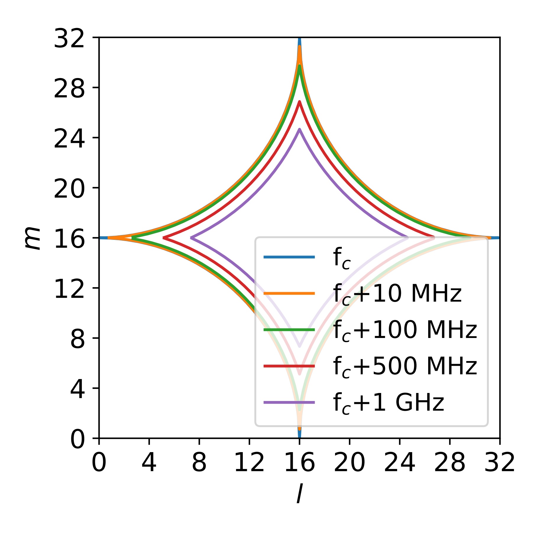
Figure 9: The boundaries between the regular and evanescent zones for different sub-carriers with $f_{c}$=10 GHz, $N_{1}=N_{2}=8$, $O_{1}=O_{2}=4$ regarding a UPA with antenna spacing of half wavelength.

TABLE III: Numbers of evanescent codewords and percentages of redundancy for different sub-carriers at 10 GHz band

Frequency	Number of evanescent codewords	Redundancy
fc	229	22.36%
fc + 10 MHz	229	22.36%
fc + 100 MHz	205	20.02%
fc + 500 MHz	161	15.72%
fc + 1 GHz	117	11.43%

VI Conclusion

The evanescent codewords in the Kronecker-product based codebooks are revealed in this paper. These codewords represent evanescent waves with spatial frequencies exceeding $k$, the spatial frequency of a plane wave in free space. Through beam pattern simulations, We have demonstrated that the evanescent codewords are incapable of generating directional beams in physical space by beam pattern simulations. Our system level simulations further confirm the redundancy of these codewords in MIMO communications. The removal of evanescent codewords is essential to improve the performance of a codebook based MIMO system. This action not only reduce the overhead in CBSR signaling but also improve the efficiency of PMI reporting. Additionally, the disabling of the evanescent codewords may alleviate the impact of noise and interference in low SINR region. For wideband communications, evanescent codewords removal should be implemented per sub-band for CBSR signaling. Evidently, there are deficiencies in Kronecker-product based codebooks, suggesting the need for new codebook design or indexing schemes in future MIMO standards. Our study also indicates that there are redundant beams when DFT-based orthogonal beams are employed in beam training and such beams should be excluded for better performance. Given the low-pass characteristics of the physical channel, modifying the Rayleigh channel model to filtering out the potential evanescent components becomes crucial.

References

- [1] E. G. Larsson, O. Edfors, F. Tufvesson and T. L. Marzetta, “Massive MIMO for next generation wireless systems,” in IEEE Communications Magazine, vol. 52, no. 2, pp. 186-195, February 2014.
- [2] Z. Qin and H. Yin, “A review of codebooks for CSI feedback in 5G new radio and beyond,” 2023, arXiv:2302.09222.
- [3] X. Fu et al., “A Tutorial on Downlink Precoder Selection Strategies for 3GPP MIMO Codebooks,” in IEEE Access, vol. 11, pp. 138897-138922, 2023.
- [4] Y. Xie, S. Jin, J. Wang, Y. Zhu, X. Gao and Y. Huang,“A limited feedback scheme for 3D multiuser MIMO based on Kronecker product codebook,” 2013 IEEE 24th Annual International Symposium on Personal, Indoor, and Mobile Radio Communications (PIMRC), London, UK, 2013, pp. 1130-1135.
- [5] J. Li et al.,“Codebook Design for Uniform Rectangular Arrays of Massive Antennas,” 2013 IEEE 77th Vehicular Technology Conference (VTC Spring), Dresden, Germany, 2013, pp. 1-5.
- [6] D. Ying, F. W. Vook, T. A. Thomas, D. J. Love and A. Ghosh,“Kronecker product correlation model and limited feedback codebook design in a 3D channel model,” 2014 IEEE International Conference on Communications (ICC), Sydney, NSW, Australia, 2014, pp. 5865-5870
- [7] Y. Wang, L. Jiang, and Y. Chen,. “Kronecker product‐based codebook design and optimisation for correlated 3D channels,” Transactions on Emerging Telecommunications Technologies, 26(11), pp. 1225-1234, 2015.
- [8] J. Suh, C. Kim, W. Sung, J. So and S. W. Heo,“Construction of a Generalized DFT Codebook Using Channel-Adaptive Parameters,” in IEEE Communications Letters, vol. 21, no. 1, pp. 196-199, Jan. 2017
- [9] Y. Huang, C. Liu, Y. Song and X. Yu, “DFT codebook-based hybrid precoding for multiuser mmWave massive MIMO systems,” EURASIP Journal on Advances in Signal Processing, 2020, 1-13.
- [10] 3rd Generation Partnership Project, “NR; Physical layer procedures for data (Release 16),” 3GPP TS 38.214, 2021, [Online]. Available: https://www.3gpp.org.
- [11] A. Pizzo, T. L. Marzetta and L. Sanguinetti, “Degrees of Freedom of Holographic MIMO Channels,” 2020 IEEE 21st International Workshop on Signal Processing Advances in Wireless Communications (SPAWC), Atlanta, GA, USA, 2020, pp. 1-5
- [12] A. Pizzo, T. L. Marzetta and L. Sanguinetti, “Spatially-Stationary Model for Holographic MIMO Small-Scale Fading,” in IEEE Journal on Selected Areas in Communications, vol. 38, no. 9, pp. 1964-1979, Sept. 2020.
- [13] A. Pizzo, A. d. J. Torres, L. Sanguinetti and T. L. Marzetta,“Nyquist Sampling and Degrees of Freedom of Electromagnetic Fields,” in IEEE Transactions on Signal Processing, vol. 70, pp. 3935-3947, 2022.
- [14] J. A. Kong, Electromagnetic Wave Theory, pp. 53-57. John Wiley & Sons, 1986.
- [15] R. Ji et al., “Extra DoF of Near-Field Holographic MIMO Communications Leveraging Evanescent Waves,” in IEEE Wireless Communications Letters, vol. 12, no. 4, pp. 580-584, April 2023.
- [16] C. A. Bennett, Principles of physical optics, pp. 78-81. John Wiley & Sons, 2008.
- [17] Lerosey, G., De Rosny, J., Tourin, A., and M. Fink, “Focusing beyond the diffraction limit with far-field time reversal,” Science, 315(5815), 1120-1122, 2007.
- [18] R. F. Harrington, Time-Harmonic Electromagnetic Fields, IEEE Press, 2001.
- [19] M. Milosevic, “On the nature of the evanescent wave,” Applied spectroscopy, 67(2), 126-131, 2013.
- [20] J. B. Pendry, L. Martin-Moreno and F. J. Garcia-Vidal, “Mimicking surface plasmons with structured surfaces,” Science, 305(5685), 847-848, 2004.
- [21] 3rd Generation Partnership Project, “Technical Specification Group Radio Access Network; Study on channel model for frequencies from 0.5 to 100 GHz (Release 16)”, 3GPP TR 38.901, 2019, [Online]. Available: https://www.3gpp.org.
- [22] J. Yang, Y. Chen, Y. Cui, Q. Wu, J. Dou and Y. Wang,“How Practical Phase-Shift Errors Affect Beamforming of Reconfigurable Intelligent Surface?,” in IEEE Transactions on Communications, vol. 71, no. 10, pp. 6130-6145, Oct. 2023.
- [23] X. Chen, S. Zhang and Q. Li, “A Review of Mutual Coupling in MIMO Systems,” in IEEE Access, vol. 6, pp. 24706-24719, 2018.
- [24] J. Yang, W. Cai and X. Wu, “A high-order time domain discontinuous Galerkin method with orthogonal tetrahedral basis for electromagnetic simulations in 3-D heterogeneous conductive media,” Communications in Computational Physics, 21(4), 1065-1089, 2017.
- [25] 3rd Generation Partnership Project, “Technical Specification Group Radio Access Network; Study on channel model for frequencies from 0.5 to 100 GHz (Release 9)”, 3GPP TR 36.814 V9.2.0, 2017, [Online]. Available: https://www.3gpp.org.
- [26] M. Cui, Z. Wu, Y. Lu, X. Wei and L. Dai, “Near-Field MIMO Communications for 6G: Fundamentals, Challenges, Potentials, and Future Directions,” in IEEE Communications Magazine, vol. 61, no. 1, pp. 40-46, January 2023.
- [27] J. An, C. Yuen, L. Dai, M. Di Renzo, M. Debbah and L. Hanzo, “Near-Field Communications: Research Advances, Potential, and Challenges,” in IEEE Wireless Communications, vol. 31, no. 3, pp. 100-107, June 2024.
- [28] A. B. Constantine, Antenna Theory: Analysis and Design. Hoboken, NJ, USA: Wiley, 2015, pp. 158–294.