Pretraining-finetuning Framework for Efficient Co-design: A Case Study on Quadruped Robot Parkour

Abstract

In nature, animals with exceptional locomotion abilities, such as cougars, often possess asymmetric fore and hind legs, with their powerful hind legs acting as reservoirs of energy for leaps. This observation inspired us: could optimize the leg length of quadruped robots endow them with similar locomotive capabilities? In this paper, we propose an approach that co-optimizes the mechanical structure and control policy to boost the locomotive prowess of quadruped robots. Specifically, we introduce a novel pretraining-finetuning framework, which not only guarantees optimal control strategies for each mechanical candidate but also ensures time efficiency. Additionally, we have devised an innovative training method for our pretraining network, integrating spatial domain randomization with regularization methods, markedly improving the network’s generalizability. Our experimental results indicate that the proposed pretraining-finetuning framework significantly enhances the overall co-design performance with less time consumption. Moreover, the co-design strategy substantially exceeds the conventional method of independently optimizing control strategies, further improving the robot’s locomotive performance and providing an innovative approach to enhancing the extreme parkour capabilities of quadruped robots.

I INTRODUCTION

Quadruped animals exhibit exceptional mobility capabilities. For instance, a cougar can leap up to 5.5 meters high, and with a run-up, it can jump 12 meters. Similarly, a red kangaroo, about 1.8 meters tall, can easily leap forward more than 9 meters, quintupling its height. Imagine if legged robots could harness similar locomotive prowess, this could significantly boost their functionality, especially in challenging environments. It is noteworthy that quadruped mammals typically exhibit an asymmetric leg structure, a result of natural evolution that favors agile movement in their natural habitats [1]. This realization spurred our curiosity: Could adjusting the leg length of standard quadruped robots potentially unlock greater locomotive capabilities?

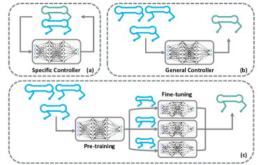
Figure 1: Comparison of co-design methods. (a) Designing distinct control strategies tailored to various morphologies, which demands considerable computational resources. (b) Utilizing a generalized strategy as a substitute, which saves time but cannot guarantee optimality. (c) The algorithm we introduce starts by training a generalized model across varying leg lengths, followed by fine-tuning for specific morphology. The fine-tuning process requires merely a small percentage of steps typically necessary, striking a balance between performance and time-saving efficacy.

The joint optimization of a robot’s mechanical structure and control policy is referred to as co-design, and currently, there are numerous works focused on the co-design of quadruped robots [2, 3, 4, 5, 6]. These studies are primarily confined to walking tasks. For instance, [2] explored the ideal proportion between upper and lower limbs, optimizing for objectives such as speed tracking and energy efficacy across varied terrains. [5] accentuated the generalizability of the transformer-based control strategy, asserting its adaptability across a myriad of leg length ratios. It also showcased that using a fixed control policy, solely morphological updates could enable a robot to step over a 10 $\mathrm{c}\mathrm{m}$ platform. [3, 4] improved the mobility of small-scale quadruped robots with limited degrees of freedom on flat ground through co-design approaches. However, the potential of robot co-design has not yet been fully realized in simple walking tasks. In more challenging control tasks like parkour tasks [7, 8, 9, 10], such as high jumping and long jumping, the significance of co-design becomes even more prominent. The physical capabilities of a robot and the scope of tasks it can execute are constrained by its hardware components. When the mechanical structure is not aptly designed, even the most ingeniously crafted motion control policies might struggle to fulfill the intended tasks. It is through a reciprocal enhancement of mechanical structure and control policies that the functional ceiling of a robot can be significantly elevated.

The co-design of robots can be primarily divided into methods based on dynamic models [11, 12, 13] and methods based on deep reinforcement learning (DRL) [2, 3, 4, 5, 6, 14, 15, 1, 16, 17]. However, dynamic model based methods require a wealth of expert knowledge and engineering experience to construct dynamical models and design equations and inequality constraints. For robots with different mechanical structures, system identification [18] must also be incorporated for motion control, which can be exceedingly tedious and complicated. DRL-based methods typically frame the problem as a bi-level optimization issue, with the lower-level optimizing the control strategy for a specified morphology and the upper-level searching for the best morphology given the optimal control policy. Depending on how the control strategy is obtained, there are mainly two categories. The first involves training specific controllers for given candidate structures during the upper-level optimization, as shown in Fig. 1(a). For instance, [1] uses a tournament algorithm at the upper-level, employing the fitness of each candidate morphology as input to derive the optimal morphology. On the lower-level, it utilizes 1152 CPUs with DRL algorithms to learn the optimal control policies for various candidate morphologies, which is highly time-consuming and requires substantial computational power. In contrast, the second category focuses on developing a versatile, generalizable model [3, 2, 5, 6], capable of offering alternative strategies for various morphologies, as depicted in Fig. 1(b). For example, [3] employs a concurrent network architecture, consisting of both individual and population networks. At the lower-level, individual networks are trained for control policies of robots with specific morphology, while at the upper-level, the population network integrates all the training data from different morphologies to achieve a generalized strategy, hence saving time by avoiding the need for separate control policies for each candidate morphology. Similarly, [6] uses the teacher-student approach, and [5] leverages a transformer architecture, both training control strategies that can generalize across different morphologies, significantly time-efficient compared to the first category methods. However, this approach of substituting optimal strategies with generalized ones for different structures, while time-saving, cannot ensure optimality in specific morphologies, potentially impairing the efficacy of upper-level optimization decisions.

In order to maintain optimality while also conserving computational power, in this paper, we introduced a pretraining-finetuning framework for quadruped robots’ co-design, with the goal of improving their parkour performance, as shown in Fig. 1(c). We first trained a parkour strategy for robots that is adaptable across a variety of leg lengths. Specifically, we integrated spatial domain randomization and regularization techniques. The former enables simultaneous training of thousands of robots with varying leg lengths, while the latter helps in reducing memory biases in the value network. The combination of them significantly enhances the generalizability of the pre-trained model. In the subsequent phase of morphology optimization, we fine-tuned this generalized model to suit each specific morphology candidate. Our experimental results indicate that merely 400 steps of fine-tuning (6.67% of the typical training steps) were sufficient for the new model to converge, delivering performance comparable to models specifically designed for each structure. In summary, the contributions of this paper are as follows:

1. We introduced a pretraining-finetuning framework to address the co-design challenge in robotics, ensuring optimality while conserving computational resources.

2. We proposed the concept of combining spatial domain randomization with regularization to obtain a pre-trained model, effectively enabling generalization across robots with different leg lengths.

3. Extensive ablation and comparative experiments have validated the efficacy of our proposed algorithm in co-design tasks, demonstrating its capability to improve the parkour performance of robots.

II Methodology

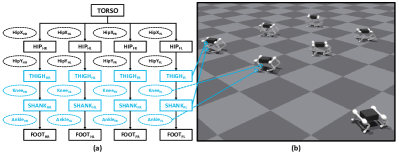
Figure 2: (a) The URDF model of the quadruped robot, where the solid rectangle represents the robot’s link, and the dashed ellipse represents the robot’s joint. The black part denotes fixed parameters, while the blue part denotes parameters that need to be changed. (b) The quadruped robot with different scaling parameters. For better comprehension, in this figure, the robots positioned further away have longer legs.

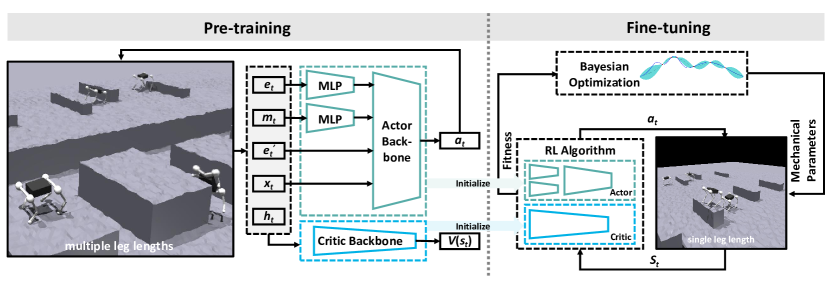
Figure 3: Overview of the proposed co-design pipeline. We initially pre-train a control strategy capable of generalizing across various morphologies. Subsequently, we embed the fine-tuning process into the morphological optimization phase, fine-tuning the pre-trained strategy for each set of candidate morphologies. This approach provides more accurate fitness values for morphological optimization. We employed the Proximal Policy Optimization (PPO) algorithm to update our policy, utilizing an asymmetric actor-critic architecture. Additionally, during the pre-training phase, we employed the technique of curriculum learning.

II-A System Overview

The overall framework of our method is depicted in Fig. 3, including two phases: Pre-training (Section II-B) and Bayesian optimization (BO) with embedded fine-tuning (Section II-C). In the first phase, we develop a parkour policy that generalizes to varying leg lengths, serving as an initial model. During the second phase, the algorithm iteratively finds the optimal morphology using the fitness of candidate morphologies as prior knowledge. Since the pre-trained model might not be optimal for every specific morphology, we fine-tune it for better accuracy. This fine-tuning allows for more precise fitness calculations in BO, improving the co-design process’s overall effectiveness.

We frame the parkour control problem as a Markov Decision Process (MDP), which is defined by a tuple $\left\langle{\mathcal{S},\mathcal{A},P,r,\gamma}\right\rangle$, in which $\mathcal{S}$ is the state space, $\mathcal{A}$ is the action space, $P(s_{t+1}|s_{t},a_{t})$ is the transition probability, $r(s_{t},a_{t})$ is the reward function, and $\gamma$ is the discount factor. At each timestep, the agent receives a state $s_{t}\in\mathcal{S}$ from the environment and selects an action $a_{t}\in\mathcal{A}$, guided by policy $\pi_{\theta}(a_{t}|s_{t})$. This action yields a reward $r_{t}$. The objective of DRL is to derive an optimal policy $\pi^{*}$ that maximizes the expected sum of discounted rewards ${\mathbb{E}}\left[{\sum_{t=0}^{T}{{\gamma^{t}}{r_{t}}}}\right]$.

Design of State and Action Space. The state comprises four parts: the proprioceptive state $x_{t}$, the explicit privileged state ${e^{\prime}_{t}}$, the privileged state $e_{t}$, the exteroceptive state $m_{t}$, and the historical proprioceptive state $h_{t}$. The $x_{t}$ includes the body’s angular velocity, roll angle, pitch angle, the difference between the body’s yaw angle and the target yaw angle, positions and velocities of joints, the actions in the previous step, and foot contact information. The $e^{\prime}_{t}$ is the body’s linear velocity. $e_{t}$ encompasses the robot’s mass, center of mass position, robot morphology parameters, friction factor, and motor strength parameters. $m_{t}$ consists of height sampling points. The action $a_{t}$ is the target angles for the robot’s twelve joints, which are converted into torques through a PD controller and then transmitted to the robot.

Design of Reward Function. Unlike previous works [19, 20, 21, 22], which utilized velocity tracking as the primary reward function item, manually specifying the robot’s linear velocity and its yaw angle in parkour tasks constraints the solution space of actions, leading to failure in performing parkour tasks. We designed our reward functions by referring to [9]. The primary reward function Goal Tracking, encourages the robot to move toward waypoint markers. When encountering an elevated platform, this reward function item motivates the robot to jump onto it rather than bypass it, as in obstacle avoidance tasks. The design of the reward function item is shown in Tab. VI of the Appendix.

II-B Pre-training Phase

TABLE I: The parameters that need to be modified in the URDF file

Tag	Attribute	Parameters	Values
Link	Inertial	Origin	x:0, y: 0, z: $\frac{{-{l_{i}}\times{\xi_{i}}}}{2}$
		Mass	value: ${m_{i}}\times{\xi_{i}}$
		Inertia	ixx: $\frac{{{m_{i}}}}{{12}}\left({b_{i}^{2}+l_{i}^{2}}\right)$
			iyy: $\frac{{{m_{i}}}}{{12}}\left({b_{i}^{2}+l_{i}^{2}}\right)$
			izz: $\frac{{{m_{i}}b_{i}^{2}}}{6}$
	Visual	Origin	x:0, y:0, z:$\frac{{-{l_{i}}\times{\xi_{i}}}}{2}$
		Geometry/Box	size: ${b_{i}},{b_{i}},{l_{i}}\times{\xi_{i}}$
	collision	Origin	x:0, y:0, z: $\frac{{-{l_{i}}\times{\xi_{i}}}}{2}$
		Geometry/Box	size: ${b_{i}},{b_{i}},{l_{i}}\times{\xi_{i}}$
Knee joint	/	Origin	x:0, y:0, z: ${z_{knee}}\times{\xi_{i,i=0,2}}$
Ankle joint	/	Origin	x:0, y:0, z:${z_{ankle}}\times{\xi_{i,i=1,3}}$

• • when $i$=0, it represents the left/right front thigh; $i$=1 corresponds to the left/right front shank; $i$=2 denotes the left/right hind thigh; and $i$=3 indicates the left/right hind shank. The variable $l_{i}$ represents the original length of each leg, while $m_{i}$ signifies the original mass of each leg. The collision model of the leg is represented by a cuboid with a square cross-section, where $b_{i}$ denotes the side length of the square cross-section. Furthermore, $z_{knee}$ represents the original position of the knee joint, and $z_{ankle}$ denotes the original position of the ankle joint.

II-B1 Spatial Domain Randomization

Domain randomization emerges as a pivotal technique for augmenting the generalization capacity of DRL models. By sampling dynamic parameters within a specified reasonable range, this method significantly enhances the model’s robustness. This approach is primarily utilized to bridge the sim2real gap [23] in DRL. Unlike previous approaches [24, 21], our approach, utilizing domain randomization, is designed to obtain a pre-trained model with exceptional generalization abilities, thus establishing a robust foundation for subsequent fine-tuning phases. In traditional practices, domain randomization has involved the alteration of variables such as friction coefficients and motor strengths during training iterations, a process we refer to as Temporal Domain Randomization. However, altering the robot’s mechanical parameters, which are predetermined at the onset of the simulator, presents a significant challenge for modifications during training. To address this, we introduce the concept of Spatial Domain Randomization. Leveraging the extensive parallel capabilities of Isaac Gym [25], we implement this innovative approach by simultaneously training thousands of robots with varied leg lengths in a single environment. This approach allows us to develop a parkour control strategy with good generalization in just a few hours.

Similar to our previous work [4], we create robots with varying morphological parameters by modifying the unified robot description format (URDF) files of the quadruped robots. The URDF of a quadruped robot is illustrated in Fig. 2(a). In this paper, we primarily focus on altering the lengths of the robot’s shanks and thighs, as indicated by the blue parts in Fig. 2(a). For each link and joint requiring modification, the specific parameters to be changed are detailed in Tab. I. To ensure the robot’s stability, we make the corresponding parts of the robot’s left and right legs symmetrical. Therefore, the adjustable parameters are the scaling factors for the front thighs, front shanks, hind thighs, and hind shanks. When training the generalizable model, we allow the scaling factors to randomly sample within a feasible range, ${\xi_{i}}\sim\mathcal{U}(c_{min},c_{max})$. The sampled parameters ${\xi_{i}}$ are then used to construct robots with varied leg lengths, as illustrated in Fig. 2(b).

II-B2 Regularizations

In the previous section, we introduced the spatial domain randomization method, which enables the algorithm to train using data from robots with varying leg lengths. As introduced in [26, 27], a value network trained across multiple agents is more likely to memorize the training data, leading to poor generalization to unvisited states. This not only hinders training performance but also negatively impacts testing performance in new environments. To mitigate this issue, we have implemented two types of regularization methods. The first method is Activation Regularization, which entails the inclusion of a regularization term in the critic’s loss function of PPO [28], as shown below:

where $\hat{A}_{t}^{\gamma}={\sum_{l=0}^{\infty}{(\gamma\lambda)}^{l}}\delta_{t+l}^{\gamma}$, this term provides an estimate of the advantage function at time step $t$ using a discount factor $\gamma$. $\lambda$ is the hyperparameter associated with Generalized Advantage Estimation (GAE) [29]. The temporal difference error $\delta_{t}^{\gamma}$ is defined as $r_{t}+\gamma V_{\phi}(s_{t+1})-V_{\phi}(s_{t})$. $\beta$ is a hyperparameter, which aims to penalize large value estimates, thereby promoting more consistent value estimation across different state-action pairs. Such a strategy potentially fosters generalization by reducing the impact of spurious approximation errors.

The second method we adopted is Discount Regularization, which is straightforward to implement. It involves adjusting the discount factor to a smaller value, denoted as ${\gamma_{{\rm{reg}}}}$, where $0\textless{\gamma_{{\rm{reg}}}}\textless\gamma\textless 1$. In this case, $\hat{R}_{t}^{\gamma}$ is replaced with $\hat{R}_{t}^{{\gamma_{{\rm{reg}}}}}$, as shown below:

$$J_{V}^{\rm{D}}(\phi)={\mathbb{E}_{{s_{t}}\sim\tau}}\left[{\frac{1}{2}{{\left({{V_{\phi}}({s_{t}})-\hat{R}_{t}^{{\gamma_{\rm{reg}}}}}\right)}^{2}}}\right]$$ (2)

A lower discount factor reduces reliance on future rewards, making the algorithm focus on short-term gains. This approach may improve generalization by reducing variance.

II-C BO with Embedded Fine-tuning

II-C1 Fine-tuning Based on Pre-trained Model

By integrating spatial domain randomization with regularization, we have developed a control strategy applicable to robots with varying leg lengths. However, this strategy does not guarantee optimality in each morphology. To provide a more reliable fitness function for the morphology optimization algorithm, each morphological candidate provided by the morphology optimization algorithm is fine-tuned. Diverging from the training of generalized models, we made three modifications: (1) The spatial domain randomization is omitted, focusing the training exclusively on the specific morphology. (2) Remove the regularizations. (3) The difficulty level of the curriculum training is elevated to the highest tier. Through these modifications, the fine-tuned control strategy is better suited for robots in the specific morphology.

II-C2 Morphology Optimization

The objective of morphology optimization is to find optimal morphology parameters $\xi\in\Xi$ for a specified parkour task $\kappa\in\mathcal{K}$ and a given control strategy $\pi\in\Pi$, such that the objective function $f(\left.\xi\right|\kappa,\pi):\Xi\times\mathcal{K}\times\Pi\to\mathbb{R}$ is maximized. This study focuses primarily on the high jump and long jump tasks, denoted as $\mathcal{K}=\left\{{{\kappa_{high}},{\kappa_{long}}}\right\}$. The optimization objective (also known as fitness) $f(\cdot)$ can be any metric, we use the robot’s non-discounted cumulative reward in a single epoch as our optimization objective, as shown below:

$$f=\frac{1}{N}\sum\limits_{i=0}^{N}{\sum\limits_{t=0}^{T}{r(s_{t}^{i},a_{t}^{i})}}$$ (3)

where $T$ denotes the number of steps in an episode, while $N$ represents the number of robots interacting with the environment. Typically, $\xi$ is non-differentiable relative to $f(\cdot)$ because legged locomotion involves many discrete changes due to foot contact. Hence, we utilize a black-box optimization method, specifically BO, for the optimization of morphology parameters. The optimization problem can be summarized as follows:

$${\xi^{*}}=\mathop{\arg\max}\limits_{\xi\in\Xi}f(\left.\xi\right|\kappa,\pi_{\xi})$$ (4)

The BO algorithm is an iterative process where, in each iteration, a candidate morphology $\xi$ is selected. Based on this chosen morphology, the RL algorithm initially fine-tuned the control policy on the basis of the pre-trained model. After deriving the strategy $\pi_{\xi}$, the robot equipped with the morphology parameters $\xi$ interacts with the environment under the guidance of $\pi_{\xi}$ to obtain $f(\cdot)$. This outcome is then fed back to the BO algorithm, which continues to iterate until a specified number of rounds are completed, ultimately yielding the optimal morphology.

III Experiments

III-A Implementation Details

During the training process, we employed Isaac Gym as the simulator. The network was built using PyTorch, and training was facilitated using Nvidia 3090 GPUs. The neural network policy generated PD targets for all motors, operating at a frequency of 50 $\mathrm{H}\mathrm{z}$. Concurrently, the PD controllers functioned at a higher frequency of 200 $\mathrm{H}\mathrm{z}$, with a $k_{p}$ set to 40 and a $k_{d}$ configured to 0.7.

During the training process, we set the number of robots (represented as $N$) to 6144. This also means that our spatial domain randomization method created $N$ different robots with varying leg lengths. Specifically, as shown in Section II-B1, during the initialization of the environment, we first select $\xi_{i,i=0,1,2,3}$ within the range $\mathcal{U}(0.6,1.4)$. After obtaining $N$ sets of $[\xi_{0},\xi_{1},\xi_{2},\xi_{3}]$ parameters, we update the original URDF files based on Tab. I to obtain $N$ sets of different URDF files, which are then loaded into the simulator.

III-B Performane of Control Policy

Comparison of Domain Randomization: To evaluate the effectiveness of spatial domain randomization (DR), we conducted three experiments for comparison.

• Temporal-DR. We varied the leg length of the robots during the training process. Since altering the leg lengths of the robot in each episode is impractical, we selected eight typical morphologies. We start training with the first set of morphologies, switching to the next set once $1/8$ of the overall process is completed, and so on, until the training concludes.

• Spatial-DR (Ours). The proposed method, involved using $N$ robots with varied morphologies to simultaneously gather data for training the policy.

• No-DR. No domain randomization strategy was employed, and all robots shared the same default morphology, i.e., $\xi_{i}=[1.0]\times 4$.

To validate the performance of three domain randomization methods, we uniformly sampled dozens of morphologies and recorded the average cumulative rewards achieved by each method under these morphologies. Furthermore, we conducted T-tests comparing the proposed method with Temporal-DR and No-DR, and the results are presented in Tab. II. It is evident that the proposed method yielded the highest mean values, and the P-values between the proposed method and the two baselines are less than the threshold of 0.05, confirming the statistical superiority over the two baselines. These findings demonstrate that the Spatial-DR method effectively enhances the generality of the control policy without necessitating extra computational resources.

TABLE II: Comparison of domain randomization methods

Methods	Temporal-DR	Spatial-DR	No-DR
Mean value	5.11$\pm$0.02	10.75$\pm$0.02	7.50$\pm$0.01
P-value	$1.18\times 10^{-9}~{}~{}~{}~{}~{}8.36\times 10^{-9}$

Comparison of Regularization: To verify the effectiveness of regularization methods, we designed the following experiments:

• Activation Regularization (A-Reg). As demonstrated by Eq. (1), we added a regularization term to the Critic’s loss function. Following numerous tests, we selected a coefficient $\beta=0.2$.

• Discount Regularization (D-Reg). As detailed by Eq. (2), we altered the discount factor $\gamma$ in the PPO algorithm to a regulated value $\gamma_{\rm reg}$. After numerous tests, we settled on $\gamma_{\rm reg}=0.98$.

• Normal. This approach does not employ regularization, retaining the original $\gamma$ value of 0.99.

• Phasic Policy Gradient (PPG) [27]. A SOTA method for enhancing the generalizability of RL algorithms. It integrates auxiliary losses during the training of the PPO algorithm to improve the algorithm’s generalizability, details can be found in [27].

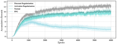
Figure 4: The curve of cumulative rewards changes with the training steps. The results presented are average across three experiments, and the shaded areas represent the variance of these experiments.

To compare the effectiveness of different regularization methods, we plotted the cumulative reward curves for each approach during the training process, as shown in Fig. 4. It is evident that D-Reg yielded the best results, followed by A-Reg, while PPG underperformed, even falling behind Normal, which doesn’t use any regularization techniques. Taking both the effectiveness and the simplicity of algorithm implementation into account, D-Reg proves to be superior in our locomotion control tasks. It is noteworthy that PPG exhibited the poorest performance. We suspect this may be because the PPG algorithm was developed for image-based RL and might not be well suited for motion control RL with low dimensional observations.

Performance of Fine-tuning: In this section, we demonstrate the effectiveness of fine-tuning, considering both the time consumption and the performance enhancements, we applied two methods as follows.

• Standard Training. Normative training under the specific morphology without pre-training.

• Fine-tuning. The proposed method, starts with pre-training using the spatial domain randomization and regularization technique, followed by fine-tuning under the specific morphology.

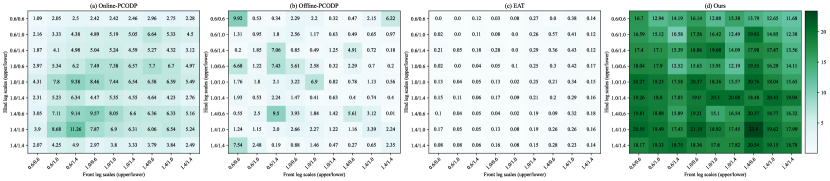
Figure 5: Heatmap of co-design experiments. Each block represents the cumulative rewards achieved using the corresponding control strategy in the parkour task under a given morphology. The $x$-axis represents the ratio factor between the thigh and the shank of the front leg, while the $y$-axis indicates the ratio factor between the thigh and shank of the hind leg. The darker the shade of each block, the higher the cumulative rewards, indicating better performance of the algorithm. For Online-PCODP, Offline-PCODP, and EAT, the eight typical morphologies used are the same as Fig. 6(b).

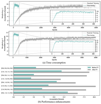
Figure 6: Fine-tuning experimental results. (a) Time consumption. The subgraph on the right is an enlarged version of the Fine-tuning curves. Each process was run three times, the solid lines represent the mean value, while the shaded areas indicate the variance. (b) shows the bar chart of cumulative rewards on eight typical morphologies before and after fine-tuning, displaying the mean results of three runs, the $y$-axis represents the eight typical morphologies.

The time comparison, illustrated in Fig. 6(a), reveals that Standard Training begins to converge at the 2000th epoch, while Fine-tuning starts converging at just the 100th epoch. These findings validate that the proposed method can significantly accelerate the training process. For instance, when training 30 specific morphologies, Standard Training requires $30\times 6000=1.8\times 10^{5}$ epochs, whereas Fine-tuning only needs $6000+30\times 400=1.8\times 10^{4}$ epochs. The number 6000 represents the pre-training steps, while 400 indicates the fine-tuning steps tailored for specific morphologies, equivalent to 6.67% of the former. Furthermore, we also compared the performance enhancements. Fig. 6(b) displays the accumulative rewards in eight typical morphologies, both using the pre-trained model (Before FT) and after fine-tuning the pre-trained model (After FT). It indicates that, in all cases, the performance of the strategies improved significantly after fine-tuning, thereby affirming the effectiveness of our proposed method in terms of performance enhancement.

III-C Comparison with Co-design Baselines

In this section, we compare the proposed method with three co-design baselines, we first introduce these methods.

• Online Policy Conditioned on Design Parameters (Online-PCODP) [6]. This method treats design parameters as privileged information and samples these parameters uniformly within their range during the training process. It assumes that near-optimal performance can be achieved using a policy conditioned on design parameters. In our parkour task, since modifying morphological parameters in each episode is impractical, we have adopted the Temporal-DR method to train the policy.

• Offline Policy Conditioned on Design Parameters (Offline-PCODP) [3]. This method collects interaction data from various morphologies using online RL and then uses offline RL to create a general policy from these data, which acts as a surrogate for optimizing the morphology. In detail, it first trains separate policies for eight typical morphological parameters with PPO, and then develops the general policy using TD3-BC [30].

• Embodiment-aware Transformer (EAT) [5]. Similar to Offline-PCODP, this approach initially focuses on training separate control policies for various morphological parameters to gather interaction data. These data are then trained using a network based on the Transformer architecture, ultimately yielding a control policy with generalization capabilities.

• Pre-training and Fine-tuning (Ours). The proposed method. We start by training an initial model with generalization, followed by fine-tuning for different morphologies.

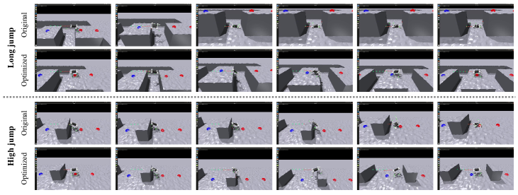
Figure 7: Comparison screenshots of different morphologies in extreme long jump and high jump tasks. For each task, the first row displays the original morphology, while the second row shows the optimized morphology. The sampling interval is 0.5$\mathrm{s}$.

We uniformly sampled 81 different morphologies from the sampling range and plotted the cumulative rewards of different methods under these morphologies in Fig. 5. As can be seen from Fig. 5(d), our proposed method achieves the highest rewards across various morphologies, demonstrating that the pre-training and fine-tuning approach can provide a more effective control strategy for the optimization of morphological parameters. For the Online-PCODP method, as observed in Fig. 5(a), its highest reward values are concentrated under the last trained morphology. For previously encountered morphologies such as the extremely short legs and extremely long legs, it shows lower cumulative rewards. These results indicate that this method is prone to forgetting previously trained morphologies, focusing instead on the final morphology. For the Offline-PCODP method, as seen in Fig. 5(b), its highest rewards are found near the eight typical morphologies encountered during training. However, for morphologies not previously encountered, it shows lower cumulative rewards, proving that this method struggles to generalize to morphologies significantly different from those seen during training. Regarding the EAT method, as seen in Fig. 5(c), its performance appears to be poor across all morphologies. We speculate that this may be due to the original EAT method focusing on simple planar walking tasks with low-dimensional states such as body linear velocity and angular velocity. Our method, on the other hand, addresses complex parkour tasks, where terrain information is crucial but results in higher state dimensionality, potentially causing Transformer-based algorithms to fail.

Furthermore, we applied the aforementioned methods for co-design in both the high jump and long jump tasks. We recorded the accumulative rewards of the optimal morphologies and their corresponding control strategies obtained by each method within a single episode, as demonstrated in Tab. III. It is evident that the proposed method achieved the highest values in both tasks, markedly surpassing the baseline methods. This substantiates the effectiveness of the proposed pretraining-finetuning framework in the context of co-design. In Tab. III, we also recorded the time consumption of various methods, wherein the time for the Online-PCODP and the proposed methods encompasses the duration for training the control strategy as well as the time for BO. The time for Offline-PCODP and EAT contains the duration for training the expert control strategy, collecting expert data, training the general network, and the time for BO. The introduction of the fine-tuning during the BO process has incurred some additional time, however, overall, the time consumed by the proposed method is still much less than that of the Offline-PCODP and EAT methods. Taking both performance and time consumption into consideration, the advantages of the proposed method are clearly notable.

TABLE III: Results of comparison with co-design baselines

	Long jump	High jump	Time Consumption
Online-PCODP [6]	9.44	14.76	3$\mathrm{h}$ 5$\mathrm{m}\mathrm{i}\mathrm{n}$
Offline-PCODP [3]	9.64	9.68	24$\mathrm{h}$ 33$\mathrm{m}\mathrm{i}\mathrm{n}$
EAT [5]	0.32	1.48	24$\mathrm{h}$ 2$\mathrm{m}\mathrm{i}\mathrm{n}$
Ours	31.49	33.25	8$\mathrm{h}$ 51$\mathrm{m}\mathrm{i}\mathrm{n}$

III-D Parkour Performance Comparison

Comparison of Single Task: In this section, we compared the performance achievable by baselines with that of the proposed approach for the tasks of long jump and high jump, as illustrated in Tab. IV. The values for the baseline methods were cited from the corresponding papers. As seen in Tab. IV, the proposed method significantly enhances the performance of robots in various parkour tasks, demonstrating that, in addition to improving the motion controller’s performance, appropriate optimization of the mechanical structure can also enhance the performance of quadruped robots in extreme tasks. Furthermore, we illustrated the performance of the robots in extreme tasks before and after morphological optimization, as shown in Fig. 7. For the long jump task, it is clear that the optimized robots are equipped with longer hind legs, which can provide more robust propulsion, while shorter front legs can assist the robot in gripping the ground ahead to prevent falls. Similarly, for the high jump task, the robots evolved to have longer legs, aiding in climbing. Both experiments underscore the potential of the co-design approach in unlocking the parkour performance of robots.

Comparison of Mixed Task: In the previous section, we conducted co-design of the robot for different tasks. In this part, we perform co-design of the robot for the mixed tasks and compare it to quadruped mammals. The crural index, the ratio of tibia (the hind shank) to femur (the hind thigh) length times 100, is higher in good jumpers, with an average crural index of 80 in humans and typically exceeding 100 in animals proficient in jumping [31]. We measured the fitness of morphologies with crural indices above and below 100 during BO, using Levene’s test and T-test for analysis. The data in Tab. V show that morphologies with higher crural indices performed better, in line with natural findings. The Levene test checks if data sets have similar variances, a value above 0.05 confirms this. We use the T-test, which assumes homogeneity of variances, to analyze the two sets of data. A P-value below 0.05 shows they are statistically different.

TABLE IV: Parkour performance comparison

	Long jump	High jump
Robot Parkour Learning[7]	0.6$\mathrm{m}$	0.4$\mathrm{m}$
Extreme Parkour[9]	0.8$\mathrm{m}$	0.5$\mathrm{m}$
Ours	1.0$\mathrm{m}$	0.55$\mathrm{m}$

TABLE V: Fitness of different crural index

Crural Index		Levene-test P-value	T-test P-value
>100	$\leq$ 100
29.177 $\pm$ 2.02	27.898 $\pm$ 1.76	0.608	0.027

IV Conclusions

In this paper, we introduced a pretraining-finetuning framework for mechanical-control co-design in robotics. During the pre-training phase, we proposed a combination of spatial domain randomization and regularization method to train a generalizable model. We embedded the fine-tuning stage within the iterative process of BO, allowing for rapid, morphology-specific learning based on the pre-trained model during each round of BO. This approach ensures the optimality of policies across different morphologies while being time-efficient. By integrating mechanical structure optimization with control policies, we have taken a significant step forward in enhancing the extreme motion capabilities of quadruped robots, opening new avenues for their application and effectiveness in diverse environments. Currently, due to limitations in hardware structure, we have not yet created a physical robot with adjustable leg lengths. In future work, we will address this issue and validate the proposed algorithm in real-world applications.

-A Reward Function

TABLE VI: Reward function elements

Reward	Equation	Weight
Goal Tracking	$\begin{array}[]{l}\min\left({\left\langle{{\mathbf{v}},\mathbf{{\hat{d}}_{w}}}\right\rangle,v^{cmd}}\right)\\ {\mathbf{{\hat{d}}_{w}}}=\frac{{\mathbf{p}-\mathbf{x}}}{{\left\|{\mathbf{p}-\mathbf{x}}\right\|}}\end{array}$	1.5
Clearance	$-\sum{{}_{i=0}^{4}{c_{i}}\cdot M\left[{{p_{i}}}\right]}$	-1.0
Yaw Tracking	$\exp\left\{{-{{\left\|{{\omega_{z}}-\omega_{z}^{des}}\right\|}_{1}}}\right\}$	0.5
Linear Velocity ($z$)	$v_{z}^{2}$	-1.0
Angular Velocity ($xy$)	$\omega_{xy}^{2}$	-0.05
Action Rate	${\left\|{{a_{t}}-{a_{t-1}}}\right\|_{2}}$	-0.1
Hip Position	${\left({{q_{hip}}-q_{hip}^{des}}\right)^{2}}$	-0.5
Joint Acceleration	${\ddot{q}^{2}}$	$-2.5\times 10^{-7}$
Joint Cosmetic	${\left({q-{q^{des}}}\right)^{2}}$	-0.04
Torque Change	${\left({{\tau_{t}}-{\tau_{t-1}}}\right)^{2}}$	$-1\times 10^{-7}$
Torque Penalty	$\tau_{t}^{2}$	$-1\times 10^{-5}$
Orientation	$g^{2}$	-1.0

• • In this description, $\mathbf{p}$ represents the subsequent waypoint, while $\mathbf{x}$ denotes the robot’s location within the world frame. The robot’s current velocity in the world frame is expressed as $\mathbf{v}\in\mathbb{R}^{2}$, and the target speed is indicated by ${v^{cmd}}\in\mathbb{R}^{1}$. The term $c_{i}$ equals 1 when the $i$-th foot is in contact with the ground. The boolean function $M$ returns 1 if the point $p_{i}$ is situated within 5$\mathrm{c}\mathrm{m}$ of an edge. Each leg’s foot position is given by $p_{i}$. The notation $\exp(\cdot)$ refers to exponential operators, and the superscript ${(\cdot)^{des}}$ is used to specify desired values. The base angular velocity is represented as $\omega\in\mathbb{R}^{3}$, and the base linear velocity as $v\in\mathbb{R}^{3}$. The actions are denoted by ${a_{t}}\in\mathbb{R}^{12}$, the joint angles by $q\in\mathbb{R}^{12}$, the joint accelerations by $\ddot{q}\in\mathbb{R}^{12}$, and the joint torques by ${\tau}\in\mathbb{R}^{12}$. Lastly, $g$ represents the gravity vector projected into the robot’s body frame.

References

- [1] A. Gupta, S. Savarese, S. Ganguli, and L. Fei-Fei, “Embodied intelligence via learning and evolution,” Nature communications, vol. 12, no. 1, p. 5721, 2021.
- [2] Á. Belmonte-Baeza, J. Lee, G. Valsecchi, and M. Hutter, “Meta reinforcement learning for optimal design of legged robots,” IEEE Robotics and Automation Letters, vol. 7, no. 4, pp. 12 134–12 141, 2022.
- [3] C. Chen, P. Xiang, H. Lu, Y. Wang, and R. Xiong, “C 2: Co-design of robots via concurrent-network coupling online and offline reinforcement learning,” in 2023 IEEE/RSJ International Conference on Intelligent Robots and Systems (IROS). IEEE, 2023, pp. 7487–7494.
- [4] C. Chen, P. Xiang, J. Zhang, R. Xiong, Y. Wang, and H. Lu, “Deep reinforcement learning based co-optimization of morphology and gait for small-scale legged robot,” IEEE/ASME Transactions on Mechatronics, 2023.
- [5] C. Yu, W. Zhang, H. Lai, Z. Tian, L. Kneip, and J. Wang, “Multi-embodiment legged robot control as a sequence modeling problem,” in 2023 IEEE International Conference on Robotics and Automation (ICRA). IEEE, 2023, pp. 7250–7257.
- [6] F. Bjelonic, J. Lee, P. Arm, D. Sako, D. Tateo, J. Peters, and M. Hutter, “Learning-based design and control for quadrupedal robots with parallel-elastic actuators,” IEEE Robotics and Automation Letters, vol. 8, no. 3, pp. 1611–1618, 2023.
- [7] Z. Zhuang, Z. Fu, J. Wang, C. G. Atkeson, S. Schwertfeger, C. Finn, and H. Zhao, “Robot parkour learning,” in Conference on Robot Learning. PMLR, 2023, pp. 73–92.
- [8] D. Hoeller, N. Rudin, D. Sako, and M. Hutter, “Anymal parkour: Learning agile navigation for quadrupedal robots,” arXiv preprint arXiv:2306.14874, 2023.
- [9] X. Cheng, K. Shi, A. Agarwal, and D. Pathak, “Extreme parkour with legged robots,” in RoboLetics: Workshop on Robot Learning in Athletics@ CoRL 2023, 2023.
- [10] N. Rudin, D. Hoeller, M. Bjelonic, and M. Hutter, “Advanced skills by learning locomotion and local navigation end-to-end,” in 2022 IEEE/RSJ International Conference on Intelligent Robots and Systems (IROS). IEEE, 2022, pp. 2497–2503.
- [11] S. Ha, S. Coros, A. Alspach, J. Kim, and K. Yamane, “Joint optimization of robot design and motion parameters using the implicit function theorem.” in Robotics: Science and systems, vol. 8, 2017.
- [12] M. Geilinger, R. Poranne, R. Desai, B. Thomaszewski, and S. Coros, “Skaterbots: Optimization-based design and motion synthesis for robotic creatures with legs and wheels,” ACM Transactions on Graphics (TOG), vol. 37, no. 4, pp. 1–12, 2018.
- [13] G. Fadini, T. Flayols, A. Del Prete, N. Mansard, and P. Souères, “Computational design of energy-efficient legged robots: Optimizing for size and actuators,” in 2021 IEEE International Conference on Robotics and Automation (ICRA). IEEE, 2021, pp. 9898–9904.
- [14] D. J. Hejna III, P. Abbeel, and L. Pinto, “Task-agnostic morphology evolution,” in International Conference on Learning Representations, 2020.
- [15] T. Wang, Y. Zhou, S. Fidler, and J. Ba, “Neural graph evolution: Towards efficient automatic robot design,” in International Conference on Learning Representations, 2018.
- [16] K. S. Luck, H. B. Amor, and R. Calandra, “Data-efficient co-adaptation of morphology and behaviour with deep reinforcement learning,” in Conference on Robot Learning. PMLR, 2020, pp. 854–869.
- [17] C. Schaff, D. Yunis, A. Chakrabarti, and M. R. Walter, “Jointly learning to construct and control agents using deep reinforcement learning,” in 2019 International Conference on Robotics and Automation (ICRA). IEEE, 2019, pp. 9798–9805.
- [18] U. Nagarajan, A. Mampetta, G. A. Kantor, and R. L. Hollis, “State transition, balancing, station keeping, and yaw control for a dynamically stable single spherical wheel mobile robot,” in 2009 IEEE International Conference on Robotics and Automation. IEEE, 2009, pp. 998–1003.
- [19] N. Rudin, D. Hoeller, P. Reist, and M. Hutter, “Learning to walk in minutes using massively parallel deep reinforcement learning,” in Conference on Robot Learning. PMLR, 2022, pp. 91–100.
- [20] A. Kumar, Z. Fu, D. Pathak, and J. Malik, “Rma: Rapid motor adaptation for legged robots,” arXiv preprint arXiv:2107.04034, 2021.
- [21] G. Ji, J. Mun, H. Kim, and J. Hwangbo, “Concurrent training of a control policy and a state estimator for dynamic and robust legged locomotion,” IEEE Robotics and Automation Letters, vol. 7, no. 2, pp. 4630–4637, 2022.
- [22] I. M. A. Nahrendra, B. Yu, and H. Myung, “Dreamwaq: Learning robust quadrupedal locomotion with implicit terrain imagination via deep reinforcement learning,” in 2023 IEEE International Conference on Robotics and Automation (ICRA). IEEE, 2023, pp. 5078–5084.
- [23] J. Tan, T. Zhang, E. Coumans, A. Iscen, Y. Bai, D. Hafner, S. Bohez, and V. Vanhoucke, “Sim-to-real: Learning agile locomotion for quadruped robots,” arXiv preprint arXiv:1804.10332, 2018.
- [24] H. Shi, B. Zhou, H. Zeng, F. Wang, Y. Dong, J. Li, K. Wang, H. Tian, and M. Q.-H. Meng, “Reinforcement learning with evolutionary trajectory generator: A general approach for quadrupedal locomotion,” IEEE Robotics and Automation Letters, vol. 7, no. 2, pp. 3085–3092, 2022.
- [25] V. Makoviychuk, L. Wawrzyniak, Y. Guo, M. Lu, K. Storey, M. Macklin, D. Hoeller, N. Rudin, A. Allshire, A. Handa et al., “Isaac gym: High performance gpu based physics simulation for robot learning,” in Thirty-fifth Conference on Neural Information Processing Systems Datasets and Benchmarks Track (Round 2), 2021.
- [26] S. Moon, J. Lee, and H. O. Song, “Rethinking value function learning for generalization in reinforcement learning,” Advances in Neural Information Processing Systems, vol. 35, pp. 34 846–34 858, 2022.
- [27] K. W. Cobbe, J. Hilton, O. Klimov, and J. Schulman, “Phasic policy gradient,” in International Conference on Machine Learning. PMLR, 2021, pp. 2020–2027.
- [28] J. Schulman, F. Wolski, P. Dhariwal, A. Radford, and O. Klimov, “Proximal policy optimization algorithms,” arXiv preprint arXiv:1707.06347, 2017.
- [29] J. Schulman, P. Moritz, S. Levine, M. Jordan, and P. Abbeel, “High-dimensional continuous control using generalized advantage estimation,” arXiv preprint arXiv:1506.02438, 2015.
- [30] S. Fujimoto and S. S. Gu, “A minimalist approach to offline reinforcement learning,” Advances in neural information processing systems, vol. 34, pp. 20 132–20 145, 2021.
- [31] C. B. Davenport, “The crural index,” American Journal of biological anthropology, vol. 17, pp. 333–353, 1933.