Enhancing Robustness and Security in ISAC Network Design: Leveraging Transmissive Reconfigurable Intelligent Surface with RSMA

Abstract

In this paper, we propose a novel transmissive reconfigurable intelligent surface (TRIS) transceiver-enhanced robust and secure integrated sensing and communication (ISAC) network. A time-division sensing communication mechanism is designed for the scenario, which enables communication and sensing to share wireless resources. To address the interference management problem and hinder eavesdropping, we implement rate-splitting multiple access (RSMA), where the common stream is designed as a useful signal and an artificial noise (AN), while taking into account the imperfect channel state information and modeling the channel for the illegal users in a fine-grained manner as well as giving an upper bound on the error. We introduce the secrecy outage probability and construct an optimization problem with secrecy sum-rate as the objective functions to optimize the common stream beamforming matrix, the private stream beamforming matrix and the timeslot duration variable. Due to the coupling of the optimization variables and the infinity of the error set, the proposed problem is a nonconvex optimization problem that cannot be solved directly. In order to address the above challenges, the block coordinate descent (BCD)-based second-order cone programming (SOCP) algorithm is used to decouple the optimization variables and solving the problem. Specifically, the problem is decoupled into two subproblems concerning the common stream beamforming matrix, the private stream beamforming matrix, and the timeslot duration variable, which are solved by alternating optimization until convergence is reached. To solve the problem, S-procedure, Bernstein’s inequality and successive convex approximation (SCA) are employed to deal with the objective function and non-convex constraints. Numerical simulation results verify the superiority of the proposed scheme in improving the secrecy energy efficiency (SEE) and the Cramér-Rao boundary (CRB).

I Introduction

In the realm of modern communications, ensuring the security and confidentiality of transmitted data is a paramount concern. While traditional cryptographic techniques have historically focused on securing data at higher protocol layers, in recent years both academia and industry have become increasingly interested in strengthening the foundation of communication systems, the physical layer, due to its ability to protect data confidentiality without relying on key distribution or encryption/decryption, as well as latency advantages over bit-level cryptographic techniques[1, 2, 3]. However, the inherent trade-offs between security, performance and compatibility, as well as the issues of signal leakage and interference management, constrain the practical deployment of physical layer security communication (PLSC) solutions in various communication scenarios[4, 5].

The reconfigurable intelligent surface (RIS), a new paradigm for enhancing the security of the physical layer of wireless networks, significantly impacts the landscape of wireless communication systems, providing opportunities to enhance data transmission and against threats[6, 7, 8]. One of the main mechanisms by which RIS contributes to physical layer security is channel conditioning, i.e., by controlling the phase shift of the reflected signals, RIS can reshape the wireless propagation environment to create favorable conditions for the desired communication links while reducing eavesdropping attempts. Z. Li et. al investigated the problem of deploying RIS to reconfigure the wireless channel and maximizing the secrecy energy efficiency under outage probability constraints and eavesdropper equipped with multi-antenna conditions, and results demonstrate the importance of optimizing the RIS phase shift to defend against eavesdropping[9]. D.-T. Do et. al deployed RIS to improve system secrecy and communication performance in response to eavesdropping attacks, and the simulation results showed that the secrecy performance can be significantly improved by increasing the number of meta-surfaces in the RIS to reduce the quality of the channel close to the eavesdropper[10]. Subsidiarily, RIS also facilitates the implementation of secure beamforming techniques that enable precise control of the directionality and strength of transmitted signals. By creating secure communication zones through beamforming techniques, the signal-to-noise ratio (SNR) can be selectively increased for legitimate users, while limiting signal leakage and blocking unauthorized reception. This not only improves spectral efficiency and signal quality, but also enhances the confidentiality of communications. H. Niu et. al investigated the problem of secure communication involving RIS active-passive beamforming, where confidential signals are sent by active refractive RIS-based transmitters, while passive reflective RIS is used to improve the user’s confidentiality performance in the presence of multiple eavesdroppers[11]. Y. Sun et. al investigated the role of RIS in improving the spectral efficiency and security of multiuser cellular networks by converting imperfect angle channel state information (CSI) to robust CSI and designing robust RIS hybrid beamforming to solve the worst-case and rate maximization problems[12]. L. Chai et. al developed a novel two-way training scheme to detect pilot spoofing attacks and a robust secure beamforming design utilizing RIS to provide secure transmission, effectively increasing the total achievable secrecy rate[13]. However, RIS is highly dependent on accurate CSI and there is a growing need for proactive sensing of potential threats in wireless environments, so further improvements in this area are essential[14].

Sensing technology is centered on playing a key role in providing situational awareness and understanding the background of the wireless environment. By collecting CSI, monitoring signal strength and anomaly detection, security mechanisms can proactively identify, localize and respond to security threats, thereby protecting communication integrity and preserving network confidentiality[15, 16, 17, 18, 19]. Z. Ren et. al investigated the secure communication sensing problem in both cases of bounded CSI errors and CSI errors conforming to a Gaussian distribution, where the base station (BS) transmits a confidential signal integrating sensing signals to the communication user, while sensing targets that may be suspected eavesdroppers[20]. The problem of sensing-assisted physical layer security is investigated in [21]. The BS first transmits omnidirectional waveforms to obtain potential Eves information, based on which a secrecy rate expression is formulated, and then, constructs the optimization problem for simultaneously maximizing the secrecy rate and minimizing the target/Eves estimation of the Cramér-Rao boundary (CRB). By improving the estimation accuracy, the sensing and security functions are mutually beneficial. H. Jia et. al considered dual-functional radar communications with spectral and energy-efficient characteristics to enhance PLSC under eavesdropper CSI uncertainty, and utilizes the CRB as a PLSC-optimized model for the sensing metric while satisfying the tolerance sensing requirement and the minimum secrecy rate per legitimate user[22]. However, interference management issues are particularly important in sensing scenarios due to malicious attacks by eavesdroppers and the mixing of sensing and communication signals.

Rate splitting multiple access (RSMA) is known to better manage interference and thus achieve higher spectral efficiency[23, 24, 25]. By shaping the transmitted waveforms and processing the received signals, RSMA can suppress interference from other signal sources and improve the SNR, thus enhancing the robustness and reliability of the radar system. In addition, the diversification of transmission signals by splitting transmission data into common and private streams makes it more difficult for potential adversaries to intercept or decipher sensitive information, while RSMA networks share common information stream and co-optimize the allocation of resources, which can be used for identifying abnormal behaviors and threats utilizing collective intelligence. In [26], an RSMA-based secure beamforming method is proposed to maximize the weighted sum-rate. Simulations show performance superiority in channel error robustness and interference management compared to the baseline. In [27], the confidentiality performance of RSMA in a multiuser multiple-input single-output system is investigated, and simulations show that by adjusting the partitioning of the messages, the proposed power allocation methodology allows for a scalable trade-off between rate effectiveness and confidentiality. Furthermore, the common stream of RSMA is used for sensing, based on which the authors construct and maximize a performance criterion for sensing, with guaranteed communication[28]. RSMA has more flexible interference management capabilities due to its additional common stream, which provides potential design freedom.

Overall, the user’s demand for data security imposes higher requirements on future network design, which is accompanied by interference management and energy consumption issues. In this paper, we employ TRIS to empower ISAC networks and provide a low-cost, low-energy architecture in which RSMA is employed to manage interference among users. To the best of our knowledge, there is few research on TRIS-enabled ISAC networks. According to the scenario requirements, an optimization problem is constructed under imperfect CSI conditions with maximizing secrecy sum-rate as the objective function, while setting secrecy outage as a constraint to further improve the secrecy of the network. The main contributions of this paper are as follows:

• We propose a time-division secure ISAC architecture. In this architecture, communication and sensing share the same wireless resources, and the wireless environment information obtained by sensing brings benefits to communication while detecting potential illegal users (IUs). To facilitate the integration of sensing and communication, we deploy a novel transmissive reconfigurable intelligent surface (TRIS) transceiver framework that utilizes time modulatin array (TMA) for simultaneous multistream communication and sensing, and innovatively exploits the common stream for RSMA as both useful signals and artificial noise, which has not been considered in previous work.

• Based on the architectural setting, we consider the problem of secure communication and detection of potentially IUs under conditions of imperfect CSI and network serving multiple legitimate users (LUs) with the presence of multiple IUs. Since accurate estimation of IU channel is quite challenging, we model the channel and estimation error of IUs in a refined way and give theoretical upper bounds on the error. Concurrently, to improve the security of the system, we consider system outage when the secrecy rate falls below a threshold.

• In response to the above problems, we construct an optimization problem taking secrecy sum-rate as the objective function and beampattern, detection probability and outage probability as the constraints. The nonconvexity of the objective function and constraints are handled by using S-procedure, Bernstein’s inequality and successive convex approximation (SCA). Finally, the optimization problem is decoupled and solved using block coordinate descent (BCD) algorithm and second order convex cone programing (SOCP) algorithm. We evaluate the performance and numerical simulations show that the proposed scheme has a minimum gain in secrecy energy efficiency (SEE) of 44% compared to traditional transceiver, confirming the superiority of the proposed scheme.

Notations: Scalars are denoted by lower-case letters, while vectors and matrices are represented by bold lower-case letters and bold upper-case letters, respectively. $|x|$ denotes the absolute value of a complex-valued scalar $x$, ${x^{*}}$ denotes the conjugate operation, and $\left\|\bf x\right\|$ denotes the Euclidean norm of a complex-valued vector $\bf x$. For a square matrix ${\bf{X}}$, ${\rm{tr}}\left({\bf{X}}\right)$, ${\rm{rank}}\left({\bf{X}}\right)$, ${{\bf{X}}^{H}}$, ${\left[{\bf{X}}\right]_{m,n}}$ and $\left\|{\bf{X}}\right\|$ denote its trace, rank, conjugate transpose, ${m,n}$-th entry, and matrix norm, respectively. ${\bf{X}}\succeq 0$ represents that ${\bf{X}}$ is a positive semidefinite matrix. In addition, ${\mathbb{C}^{M\times N}}$ denotes the space of ${M\times N}$ complex matrices. $j$ denotes the imaginary element, i.e., $j^{2}=-1$. The distribution of a circularly symmetric complex Gaussian (CSCG) random vector with mean $\mu$ and variance $\sigma^{2}$ is denoted by ${\cal C}{\cal N}\left({{\mu},\sigma^{2}}\right)$ and $\sim$ stands for ‘distributed as’. ${\bf{A}}\otimes{\bf{B}}$ represents the Kronecker product of matrices ${\bf{A}}$ and ${\bf{B}}$.

II System Model

In this section, we first present a model of the ISAC network employing the TRIS transmitter and give the sensing mechanism. Next, based on the characteristics of this transmitter, the corresponding channel models are established and the imperfect knowledge of CSI of LUs and IUs is taken into account. Finally, the corresponding signal models are given.

Figure 1: TRIS transceiver empowered ISAC networks.

II-A ISAC Network Models

We consider a downlink multiuser ISAC system consisting of a TRIS-empowered BS with $K$ LUs and $M$ IUs, as shown in Fig. 1. The BS consists of a TRIS with $N={N_{r}}\times{N_{c}}$ elements arranged in a uniform planar array (UPA) pattern, a horn antenna and a controller, while LUs and previously detected IUs are single antenna devices.

Since this paper uses a new type of transmitter, the precoding matrix needs to meet the design requirements of the transmitter. Based on literature [30], the transmit signal is modulated on positive and negative 1st harmonics, there will be a power loss of 0.91 dB, and the power of the signal loaded on the TRIS element cannot exceed the power of the harmonics, so the power constraints need to satisfy the following expression.

$${{{\left[{{{\bf{W}}\left[l\right]}{\bf{W}}^{H}\left[l\right]}\right]}_{nn}}}\leq{P_{t}},\forall n,$$ (1)

where ${\bf{W}}\left[l\right]$ denotes the beam matrix in time slot $l$, and the maximum available power of each TRIS element is $P_{t}$. The reason that the power constraint is written as Eq. (1) is that in the TMA modulation process, the complex value of each element $x_{n}=A_{n}e^{j\varphi_{n}}$ of the signal ${\bf x}\left[l\right]={\bf W}\left[l\right]{\bf s}\left[l\right]\in\mathbb{C}^{N\times l}$ is first modulated to the 1st harmonic according to Eqs. (2) and (3), then transformed to a temporal waveform, and finally loaded onto the TRIS elements. Therefore it is required that the power of element $x_{n}$ should not exceed the power of the 1st harmonic. Based on the matrix multiplication rules, this requires constraints on the rows of the precoding matrix.

$$A_{n}/{A_{\max}}=\sin\left({\pi\tau_{n}/{T_{p}}}\right),$$ (2)

and

$$-\pi\left({2{t_{on,n}}+\tau_{n}}\right)/{T_{p}}={\varphi_{0,n}}+2k\pi,\forall k,$$ (3)

where ${T_{p}}$ is the code element time, ${A_{\max}}$ is the maximum amplitude of the modulated signal, $t_{on,n}$ denotes the moment of 0-state onset, and $\tau_{n}$ indicates the duration of the 0 state. The principle and mapping process are shown in Fig. 2.

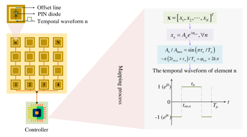
Figure 2: The principle and mapping process of TRIS.

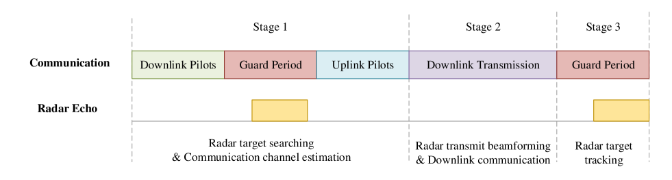
Figure 3: Frame structure of the ISAC network.

Regarding the secure ISAC mechanism, its frame structure can be divided into three stages as shown in Fig. 3. (1) Radar target searching and communication channel estimation: In this stage, the BS first transmits an omnidirectional waveform containing the downlink pilots, and then estimates the parameters such as angle of arrival, distance, and Doppler in the echo while detecting all targets. Next, the LUs receive the probing signal and estimates the departure of angle and send the uplink pilots to the BS. Finally, the BS can obtain the channel parameters and detect active LUs as well as potential IUs. (2) Radar transmit beamforming and downlink communication: In this stage, the BS has acquired the CSI containing the angle information and sends the beam in the direction of interest through the co-design of the communication-sensing beamformer for further detection of potentially IUs and downlink communication. (3) Radar target tracking: In this stage, the BS receives the echoes from the previous stage to update the target parameters. In this paper, we focus on stage 2, where the BS transmits a total of ${\cal L}=\left\{1,\cdots,L\right\}$ beam sequences at different frames and scans a sector during scanning period $T$ to downlink communication while detecting potential new IUs.

II-B Channel Model

The communication channel ${{\bf{h}}_{k}\left[l\right]}\in{\mathbb{C}^{N\times 1}}$ between the LU $k$ and the BS consists of a line-of-sight (LoS) portion and a non-line-of-sight (NLoS) portion, which can be modeled as the following Rician fading channel

$${{\bf{h}}_{k}}\left[l\right]={\xi_{k}}\left[l\right]\left({\sqrt{\frac{{{\kappa_{v}}}}{{{\kappa_{v}}+1}}}{\overline{\bf{h}}_{k}}\left[l\right]+\sqrt{\frac{1}{{{\kappa_{v}}+1}}}{\underline{\bf{h}}_{k}}\left[l\right]}\right),\forall k,$$ (4)

where ${\xi_{k}\left[l\right]={{\lambda_{c}}}/{{4\pi{d_{k}}\left[l\right]}}}$ denotes the path loss and ${\kappa_{v}}$ represents the Rician factor. ${\lambda_{c}}$ represents the carrier wavelength, and ${d_{k}}\left[l\right]$ represents the distance between the LU $k$ and the BS. The LoS channel can be expressed as

$${\overline{\bf{h}}_{k}}\left[l\right]={\left[{{e^{-j2\pi{\delta_{r}}{{\bf{n}}_{r}}}}}\right]^{T}}\otimes{\left[{{e^{-j2\pi{\delta_{c}}{{\bf{n}}_{c}}}}}\right]^{T}},\forall k,$$ (5)

where ${{\bf{n}}_{r}}=\left[{0,1,\cdots,{N_{r}}-1}\right]$, ${{\bf{n}}_{c}}=\left[{0,1,\cdots,{N_{c}}-1}\right]$, ${\delta_{r}}={{d_{f}}\sin{\theta_{k}}\left[l\right]\cos{\varphi_{k}}\left[l\right]}/{\lambda_{c}}$, and ${\delta_{c}}={{d_{f}}\sin{\theta_{k}}\left[l\right]\sin{\varphi_{k}}\left[l\right]}/{\lambda_{c}}$. $\left({{n_{r}},{n_{c}}}\right)$ denotes the element position index of the RIS and ${d_{f}}$ denotes the center distance of adjacent RIS elements. ${\varphi_{k}}\left[l\right]$ and ${\theta_{k}}\left[l\right]$ denote the user’s azimuth and pitch angles, respectively. The NLoS channel obeys a CSCG distribution, i.e., ${\underline{\bf{h}}_{k}}\left[l\right]\sim{\cal C}{\cal N}\left({0,{{\bf{I}}_{N}}}\right)$.

In addition, there is often uncertainty in the channel due to user movement, scattering from the surrounding environment, and scanning period, and in order to portray this uncertainty, an uncertainty model is used to quantify the error in the channel. The channel error vector for the LU $k$ can be expressed as

$$\Delta{{\bf{h}}_{k}}\left[l\right]={{\bf{h}}_{k}}\left[l\right]-{\widehat{\bf{h}}_{k}},\forall k,$$ (6)

where ${\widehat{\bf{h}}_{k}}$ denotes the estimated channel of LU $k$ before the scanning period and ${{\bf{\hat{h}}}_{k}}$ and $\Delta{{\bf{h}}_{k}}\left[l\right]\sim{\cal C}{\cal N}\left({0,{{\sigma_{h_{e}}^{2}}{\bf{I}}_{N}}}\right)$ are independent. ${\widehat{\bf{h}}_{k}}$ can be characterized by Eq. (4) and is assumed to be known by the BS, and can be obtained by the CSI algorithm[31]. For LUs, who interact with the BS before beam scanning, more accurate CSI can be obtained therefore $\Delta{{\bf{h}}_{k}}\left[l\right]$ is usually bounded, which can be constrained by the bounded uncertainty model, i.e., $\left\|\Delta{{\bf{h}}_{k}}\left[l\right]\right\|\leq{\varepsilon_{k}}\left[l\right],\forall k$.

Generally speaking, the BS does not know the channel information of the IUs, including their position and angle, but since the BS is able to detect potential IUs, it has knowledge of the LoS channel, which is often imprecise, including the distance and angle of the potential IUs. Meanwhile, due to the presence of scatterers in the environment and multipath fading, the NLoS channel of an IU is usually unknown, and in this paper it is assumed that its elements are bounded by an upper boundary, i.e., $\left|{\underline{g}}_{m,n}\left[l\right]\right|\leq{\varepsilon_{m,n}\left[l\right]}$. For IUs, the channel uncertainties we consider include the distance between the IU and the BS, and the azimuth and pitch angles of the IU, so the wiretap channel ${{\bf{g}}_{m}\left[l\right]}\in{\mathbb{C}^{N\times 1}}$ between a potential IU and the BS can be represented as shown in Eq. (7) at the top of the next page.

$${{\bf{g}}_{m}}\left[l\right]=\sqrt{\frac{{{\lambda^{2}_{c}}}}{{(4\pi)^{2}\left({1+{\kappa_{v}}}\right){{\left({{\widehat{d}_{m}}+\Delta{d_{m}}\left[l\right]}\right)}^{2}}}}}\left[{\sqrt{{\kappa_{v}}}{\left[{{e^{-j2\pi{{\overline{\delta}}_{r}}{{\bf{n}}_{r}}}}}\right]^{T}}\otimes{\left[{{e^{-j2\pi{{\overline{\delta}}_{c}}{{\bf{n}}_{c}}}}}\right]^{T}}+{\underline{\bf{g}}_{m}}\left[l\right]}\right],\forall m,$$ (7)

The $\Delta d_{m}\left[l\right]$ denotes the distance uncertainty and satisfies $\left|{\Delta{d_{m}}\left[l\right]}\right|\leq{D_{m}}\left[l\right].$ Meanwhile, the ${\bar{\delta}_{r}}$ and ${\bar{\delta}_{r}}$ can be expressed as

$${{\overline{\delta}}_{r}}={d_{f}}\sin\left({\widehat{\theta}_{m}}+{\Delta\theta_{m}\left[l\right]}\right)\cos\left({\widehat{\varphi}_{m}}+{\Delta\varphi_{m}\left[l\right]}\right)/{\lambda_{c}},$$ (8)

$${{\overline{\delta}}_{c}}={d_{f}}\sin\left({\widehat{\theta}_{m}}+{\Delta\theta_{m}\left[l\right]}\right)\sin\left({\widehat{\varphi}_{m}}+{\Delta\varphi_{m}\left[l\right]}\right)/{\lambda_{c}},$$ (9)

where $\left|{\Delta{\theta_{m}}\left[l\right]}\right|\leq{\Theta_{m}}\left[l\right]$ and $\left|{\Delta{\varphi_{m}}\left[l\right]}\right|\leq{\Phi_{m}}\left[l\right]$ denote the angle uncertainties. The uncertainty terms about $\Delta d_{m}\left[l\right]$, $\Delta\theta_{m}\left[l\right]$ and $\Delta\varphi_{m}\left[l\right]$ are tricky for the secure ISAC design, and in order to address thses problems, we handle them in Section IV. For ease of expression, we collect these uncertainties into the set

$$\begin{split}{\Xi_{m}}\left[l\right]\buildrel\Delta\over{=}\left\{{\left|{{\underline{g}_{m,n}}\left[l\right]}\right|\leq{\varepsilon_{m,n}}\left[l\right],\left|{\Delta{d_{m}}\left[l\right]}\right|\leq{D_{m}}\left[l\right],}\right.\\ \left.{\left|{\Delta{\theta_{m}}\left[l\right]}\right|\leq{\Theta_{m}}\left[l\right],\left|{\Delta{\varphi_{m}}\left[l\right]}\right|\leq{\Phi_{m}}\left[l\right]}\right\}.\end{split}$$ (10)

II-C Signal Model

In this paper, rate split signaling is considered where the transmission information is categorized into common and private streams. The signal can be expressed as

$$\begin{split}{\bf{x}}\left[l\right]&={{\bf{W}}\left[l\right]{\bf{s}}\left[l\right]},\\ &=\underbrace{{{\bf{w}}_{c}}\left[l\right]{s_{c}}\left[l\right]}_{{\rm{Interference~{}for~{}IU}}}+{\sum\nolimits_{i=1}^{K}{{{\bf{w}}_{i}}\left[l\right]{s_{i}}\left[l\right]}},\end{split}$$ (11)

where ${\bf{W}}\left[l\right]=\left[{{{\bf{w}}_{c}}\left[l\right],{{\bf{w}}_{1}}\left[l\right],{{\bf{w}}_{2}}\left[l\right],\cdots,{{\bf{w}}_{k}}}\left[l\right]\right]\in\mathbb{C}{{}^{N\times\left({K+1}\right)}}$ denotes the linear beamforming matrix, and ${\bf{s}}\left[l\right]={\left[{{s_{c}\left[l\right]},{s_{1}\left[l\right]},{s_{2}\left[l\right]},\cdots,{s_{K}\left[l\right]}}\right]^{T}}\in\mathbb{C}{{}^{\left({K+1}\right)\times 1}}$ represents the transmission information, which is a wide stationary process in the time domain, statistically independent and with zero mean. In this paper, the common information of all LUs are combined and jointly encoded into a common stream $s_{c}$ using the codebook codes shared by all LUs. The private information of all LUs are encoded independently as private streams $\left\{{s_{1}},\cdots,{s_{K}}\right\}$, which are only decoded by the corresponding user. For LU, the common stream is used for communication and is friendly because they can decode this part of the information. For IUs, the common stream is considered as AN and cannot be decoded.

In addition, it is reasonable and effective for the common stream to be used to interfere with the IUs due to the fact that prior to the scanning period, the LUs interact with the BS, which schedules the LUs, and the common stream encoding and decoding codebooks are shared between the LUs and the BS, and the IUs do not interact with the BS to obtain the codebook jointly encoded by the common stream, and therefore the IUs are unable to decode the information.

The signal received by the $k$-th LU can be expressed as

$${y_{k}\left[l\right]}=\sum\nolimits_{i=1}^{\cal\hat{K}}{\bf{h}}_{k}^{H}\left[l\right]{{{\bf{w}}_{i}}}\left[l\right]{{s_{i}}\left[l\right]}+{n_{k}\left[l\right]},\forall k,$$ (12)

where ${n_{k}\left[l\right]}\sim{\cal C}{\cal N}\left({0,{\sigma_{{n_{k}}}^{2}}}\right)$ denotes the Gaussian white noise at the LU and ${\cal\hat{K}}=\left\{c,1,...,K\right\}$.

The signal received by the $m$-th IU can be expressed as

$${y_{m}\left[l\right]}=\underbrace{{\bf{g}}_{m}^{H}\left[l\right]{{\bf{w}}_{c}}\left[l\right]{s_{c}}\left[l\right]}_{{\rm{AN}}}+\sum\limits_{i=1}^{K}{\bf{g}}_{m}^{H}\left[l\right]{{{\bf{w}}_{i}}}\left[l\right]{{s_{i}}\left[l\right]}+{v_{m}\left[l\right]},\forall m,$$ (13)

where ${v_{m}\left[l\right]}\sim{\cal C}{\cal N}\left({0,{\sigma_{{v_{m}}}^{2}}}\right)$ denotes the Gaussian white noise at the IU.

III Quality of Service Evaluation Metrics And Problem Formulation

In this section, we define the performance metrics for secure communication and sensing, respectively. And formulate the robust secure ISAC resource allocation optimization problem.

III-A Secure Communication Performance Metric

In this paper, we consider system secrecy sum-rate and outage probabilities as performance criteria for secure communication. The secrecy rate is designed to meet the rate requirements of LUs, and the secrecy outage probability is designed to minimize eavesdropping by IUs.

For the secrecy rate, due to the utilization of rate-spliting signaling, when LUs decoding the common stream, the private stream is considered as interference. After decoding the common stream, this part is removed in the received signal and the remaining private stream is considered as interference for decoding the current LU’s information. Then, the corresponding common and private stream signal-to-noise ratio (SNR) of the $k$-th LU can be expressed as follows

$${\gamma_{c,k}}\left[l\right]=\frac{{{{\left|{{\bf{h}}_{k}^{H}\left[l\right]{{\bf{w}}_{c}}\left[l\right]}\right|}^{2}}}}{{\sum\nolimits_{i=1}^{K}{{{\left|{{\bf{h}}_{k}^{H}\left[l\right]{{\bf{w}}_{i}}\left[l\right]}\right|}^{2}}}+{\sigma_{{n_{k}}}^{2}}}},\forall k,$$ (14)

and

$${\gamma_{p,k}}\left[l\right]=\frac{{{{\left|{{\bf{h}}_{k}^{H}\left[l\right]{{\bf{w}}_{k}}\left[l\right]}\right|}^{2}}}}{{\sum\nolimits_{i\neq k}^{K}{{{\left|{{\bf{h}}_{k}^{H}\left[l\right]{{\bf{w}}_{i}}\left[l\right]}\right|}^{2}}}+{\sigma_{{n_{k}}}^{2}}}},\forall k,$$ (15)

Then the corresponding achievable rate can be expressed as

$${R_{i,k}}\left[l\right]={\log_{2}}\left({1+{\gamma_{i,k}}\left[l\right]}\right),i\in\left\{{c,p}\right\},\forall k.$$ (16)

As mentioned earlier, the common stream is shared by all LUs and jointly participates in the encoding of the information. In order to ensure that all LUs are able to decode the common stream, the following constraints need to be satisfied

$${R_{c}}\left[l\right]=\min\left({{R_{c,1}}\left[l\right],\cdots,{R_{c,K}}}\left[l\right]\right),$$ (17)

and

$$\sum\nolimits_{k=1}^{K}{{C_{k}}\left[l\right]}={R_{c}\left[l\right]},$$ (18)

where ${C_{k}\left[l\right]}$ denotes the equivalent common stream rate of the $k$-th LU. Let ${\bf c}\left[l\right]=\left\{C_{1}\left[l\right],\cdots,C_{K}\left[l\right]\right\}$ denotes the common stream vector. Then the achievable rate for the $k$-th LU can be expressed as

$$R_{k}\left[l\right]=C_{k}\left[l\right]+R_{p,k}\left[l\right],\forall k.$$ (19)

In this paper we consider the worst-case scenario where an IU can eliminate the private stream interference from the remaining LUs before decoding the information of a specific LU. As mentioned earlier, since the IU cannot decode the common stream as AN, in the time slot $l$, the eavesdropping signal-to-noise ratio of the $m$-th IU to the $k$-th LU can be expressed as

$${\gamma_{k,m}}\left[l\right]=\frac{{{{\left|{{{\bf{g}}_{m}^{H}}\left[l\right]{{\bf{w}}_{k}}}\left[l\right]\right|}^{2}}}}{{{{{\left|{{{\bf{g}}_{m}^{H}}\left[l\right]{{\bf{w}}_{c}}\left[l\right]}\right|}^{2}}}+{\sigma_{{v_{m}}}^{2}}}},\forall k,\forall m,$$ (20)

Then the corresponding eavesdropping rate of the $m$-th IU on the $k$-th LU can be expressed as

$${R_{k,m}}\left[l\right]={\log_{2}}\left({1+{\gamma_{k,m}}\left[l\right]}\right),\forall k,\forall m,$$ (21)

Therefore, the system secrecy sum-rate in time slot $l$ can be expressed as

$$R_{tot}^{secure}\left[l\right]=\sum\nolimits_{k=1}^{K}\left[R_{k}\left[l\right]-\mathop{\rm{max}}\limits_{m\in M}R_{k,m}\left[l\right]\right]^{+},\forall l,$$ (22)

where $\left[x\right]^{+}$ denotes ${\rm max}\left\{0,x\right\}$.

For the outage probability, this paper considers two cases. The first case is considered on the LU side, which can be written in the following form

$$\Pr\left\{{{R_{k}}\left[l\right]\geq r_{k}^{s}}\right\}\geq 1-{P_{out,1}},\forall k,$$ (23)

This rate outage constraint emphasizes service reliability, i.e., it guarantees that LU $k$ can still decode rate $r_{k}^{s}$ with probability $1-{P_{out,1}}$ under the channel state information error. The second case is considered on the IU side and can be written in the following form

$$\Pr\left\{{{R_{k,m}}\left[l\right]\leq r_{m}^{e}}\right\}\geq 1-{P_{out,2}},\forall k,m,$$ (24)

This constraint ensures that the probability that the eavesdropping rate of an IU is less than a certain threshold $r_{m}^{e}$ is not less than $1-{P_{out,2}}$.

III-B Sensing Performance Metric

In general, evaluations of ISAC systems can be categorized into two types, namely, information-based metrics and estimation-based metrics. Information-based metrics include radar mutual information, etc. Estimation-based metrics include CRB, mean square error (MSE) and detection probability, etc. As above mentioned, the BS detects potential IUs, which requires the appropriate target detection performance metrics. Moreover, the BS transmits an integrated waveform for sensing and communication, so in this paper, we adopt the detection probability and beampattern approximation as the performance metrics.

The probability of detection of a potentially IU in the current time slot $l$ can be expressed in the following form

$${P_{m}^{detection}}\left[l\right]=1-{F_{{\cal X}_{\left(2\right)}^{2}}}\left({\frac{{{{2\delta}\mathord{\left/{\vphantom{{2\delta}{\sigma_{r}^{2}}}}\right.\kern-1.2pt}{\sigma_{r}^{2}}}}}{{1+p_{m}\left[l\right]{\varsigma_{m}\left[l\right]}}}}\right),\forall l,$$ (25)

where ${F_{{\cal X}_{\left(2\right)}^{2}}}$ denotes the cumulative distribution function of the chi-square distribution, $\delta=\frac{{\sigma_{r}^{2}}}{2}F_{{\cal X}_{\left(2\right)}^{2}}^{-1}\left({1-{P_{FA}}}\right)$ denotes the threshold, ${P_{FA}}$ denotes the false alarm probability, $p_{m}\left[l\right]={\rm{tr}}\left({{\bf{w}}_{c}}\left[l\right]{{\bf{w}}_{c}^{H}}\left[l\right]+{{\bf{w}}_{k}}\left[l\right]{{\bf{w}}_{k}^{H}}\left[l\right]\right)$, and ${\sigma_{r}^{2}}$ denotes processing noise. The normalized sensing channel gain $\varsigma_{m}\left[l\right]$ can be expressed as[32, 28]

$${\varsigma_{m}}\left[l\right]={\sigma_{{\alpha_{m}}}^{2}{\left|{{\bf{c}}}{\widehat{\bf{c}}^{H}}\right|^{2}}}/{N^{2}{\sigma_{r}^{2}}},\forall l,$$ (26)

where ${\alpha_{m}}\sim{\cal C}{\cal N}\left({0,\sigma_{{\alpha_{m}}}^{2}}\right)$ denotes the complex reflection coefficient, $\sigma_{{\alpha_{m}}}^{2}={S_{RCS}}{\lambda_{c}}^{2}/{((4\pi)^{3}d_{m}^{4})}$, and ${S_{RCS}}$ denotes the RCS of target. ${{\bf{c}}}=b{\bf{a}}^{H}{\left({{\theta_{m}}\left[l\right],{\varphi_{m}}\left[l\right]}\right)}$ and ${\widehat{\bf{c}}}={\widehat{b}}{\bf{\widehat{a}}}^{H}{\left({{\widehat{\theta}_{m}}\left[l\right],{\widehat{\varphi}_{m}}\left[l\right]}\right)}$ denote the radar channel steering vector and the estimated radar channel steering vector, respectively. The steering vectors can be given by the following equation

$${\bf{a}}{\left({{\theta_{m}}\left[l\right],{\varphi_{m}}\left[l\right]}\right)}={\left[{{e^{-j2\pi{{\overline{\delta}}_{r}}{{\bf{n}}_{r}}}}}\right]^{T}}\otimes{\left[{{e^{-j2\pi{{\overline{\delta}}_{c}}{{\bf{n}}_{c}}}}}\right]^{T}},$$ (27)

and

$$b={e^{-j2\pi{d_{m}}/\lambda_{c}}}.$$ (28)

As mentioned in the previous discussion, in order to ensure high quality perception of IUs, the BS utilizes a pre-designed high directional integration waveform to detect potential IUs within time slot $l$. Therefore, the following desired waveform needs to be designed.

$$\left\|{\sum\nolimits_{i=1}^{\hat{\cal K}}{{{\bf{W}}_{i}}\left[l\right]}-{\bf{R}}\left[l\right]}\right\|_{F}^{2}\leq\delta\left[l\right],\forall l,$$ (29)

where ${\bf{R}}\left[l\right]$ denotes the covariance matrix of the desired waveform[33] and $\delta\left[l\right]$ denotes the pre-designed error between the actual signal transmitted and the pre-designed high directional beampattern.

III-C Problem Formulation

In this present paper, an optimization problem is constructed to maximize the secrecy sum-rate as the objective function while guaranteeing the sensing performance as the constraints over $L$ time slots in the scanning period $T$. First we define ${\bf W}_{k}\left[l\right]={\bf w}_{k}\left[l\right]{\bf w}_{k}^{H}\left[l\right]$ and ${\bf W}_{c}\left[l\right]={\bf w}_{c}\left[l\right]{\bf w}_{c}^{H}\left[l\right]$, then design the optimization variables $\left\{t\left[l\right],C_{k}\left[l\right],{\bf W}_{k}\left[l\right],{\bf W}_{c}\left[l\right]\right\}$ by solving the following optimization problem

$$\left({{\rm{P0}}}\right){\rm{:~{}}}{\mathop{\max}\limits_{t\left[l\right],{C_{k}}\left[l\right],{{\bf{W}}_{k}}\left[l\right],{{\bf{W}}_{c}}\left[l\right]}}{\widetilde{R}_{tot}^{secure}},$$

$$~{}~{}~{}~{}~{}~{}~{}~{}~{}~{}~{}~{}~{}{\rm{s}}{\rm{.t}}{\rm{.}}~{}~{}~{}{\rm{rank}}\left({{{\bf{W}}_{i}}\left[l\right]}\right)=1,\forall i\in\hat{\cal K},\forall l,$$ (30a)

$$~{}~{}~{}~{}~{}~{}~{}~{}~{}~{}~{}~{}~{}~{}~{}~{}~{}~{}~{}~{}{{\bf{W}}_{i}}\left[l\right]\succeq 0,\forall i\in\hat{\cal K},\forall l,$$ (30b)

$$~{}~{}~{}~{}~{}~{}~{}~{}~{}~{}~{}~{}~{}~{}~{}~{}~{}~{}~{}~{}{\sum\nolimits_{i=1}^{\hat{\cal K}}{\left[{{{\bf{W}}_{i}}\left[l\right]}\right]}_{nn}}\leq{P_{t}},\forall n,l,$$ (30c)

$$~{}~{}~{}~{}~{}~{}~{}~{}~{}~{}~{}~{}~{}~{}~{}~{}~{}~{}~{}~{}\sum\nolimits_{l=1}^{L}{t\left[l\right]}\leq T,$$ (30d)

$$~{}~{}~{}~{}~{}~{}~{}~{}~{}~{}~{}~{}~{}~{}~{}~{}~{}~{}~{}~{}{t_{\min}}\leq t\left[l\right]\leq{t_{\max}},\forall l,$$ (30e)

$$~{}~{}~{}~{}~{}~{}~{}~{}~{}~{}~{}~{}~{}~{}~{}~{}~{}~{}~{}~{}{C_{k}}\left[l\right]\geq 0,\forall k,l,$$ (30f)

$$~{}~{}~{}~{}~{}~{}~{}~{}~{}~{}~{}~{}~{}~{}~{}~{}~{}~{}~{}~{}\sum\nolimits_{k=1}^{K}{{C_{k}}\left[l\right]}\leq{R_{c}}\left[l\right],\forall l,$$ (30g)

$$~{}~{}~{}~{}~{}~{}~{}~{}~{}~{}~{}~{}~{}~{}~{}~{}~{}~{}~{}~{}\Pr\left\{{{R_{k}}\left[l\right]\geq r_{k}^{s}}\right\}\geq 1-{P_{out,1}},\forall k,l,$$ (30h)

$$~{}~{}~{}~{}~{}~{}~{}~{}~{}~{}~{}~{}~{}~{}~{}~{}~{}~{}~{}~{}\Pr\left\{{{R_{k,m}}\left[l\right]\leq r_{m}^{e}}\right\}\geq 1-{P_{out,2}},\forall k,m,l,$$ (30i)

$$~{}~{}~{}~{}~{}~{}~{}~{}~{}~{}~{}~{}~{}~{}~{}~{}~{}~{}~{}~{}P_{m}^{detection}\left[l\right]\geq{P_{D}},\forall m,l,$$ (30j)

$$~{}~{}~{}~{}~{}~{}~{}~{}~{}~{}~{}~{}~{}~{}~{}~{}~{}~{}~{}~{}\left\|{\sum\nolimits_{i=1}^{\widehat{K}}{{{\bf{W}}_{i}}\left[l\right]}-{\bf{R}}\left[l\right]}\right\|_{F}^{2}\leq\delta\left[l\right],\forall l.$$ (30k)

Since space is limited, the objective function ${\widetilde{R}_{tot}^{secure}}$ is represented as shown in Eq. (31). It can be seen that problem (P0) is a nonconvex problem, due to the coupling ofvariables and nonconvex operations. In next section, we will discuss how to transform it into a convex problem and solve it.

$${\widetilde{R}_{tot}^{secure}}={\frac{1}{T}}\sum\nolimits_{l=1}^{L}{t\left[l\right]}\sum\nolimits_{k=1}^{K}{{{\left[{\mathop{\min}\limits_{\Delta{{\bf{h}}_{k}}\left[l\right]}{R_{k}}\left[l\right]}-{\mathop{{\rm{max}}}\limits_{m\in M}{\mathop{\max}\limits_{{\Xi_{m}}\left[l\right]}{R_{k,m}}\left[l\right]}}\right]}^{+}}}.$$ (31)

IV Joint Design of Communication and Sensing

In this section, we first give the bound for uncertainty region of IUs’ channel, and then the above non-convex problem (P0) is transformed into a convex problem and solved, along with the joint design of communication and sensing parameters, and finally the complexity and convergence analysis of the algorithm is given.

IV-A Bound for IUs’ Channel Error

We consider the angle and the small-scale fading uncertainties of IUs’ channel. The ${\bf g}_{m}\left[l\right]$ in (7) can be rewrited as

$$\begin{split}{{\bf{g}}_{m}}\left[l\right]&=\sqrt{\frac{{\xi_{m}^{2}\left[l\right]}}{{\left({1+{\kappa_{v}}}\right)}}}\left[{\sqrt{{\kappa_{v}}}+\Delta{g_{m,1}}\left[l\right],}\right.\\ &~{}~{}~{}~{}~{}~{}~{}~{}~{}~{}~{}\left.{\cdots,\sqrt{{\kappa_{v}}}{e^{-j{\psi_{m,N}}\left[l\right]}}+\Delta{g_{m,N}}\left[l\right]}\right]^{T},\end{split}$$ (32)

where $\xi_{m}\left[l\right]={{\lambda_{c}}}/{{4\pi{d_{m}}\left[l\right]}}$, ${d_{m}}\left[l\right]={{\widehat{d}_{m}}+\Delta{d_{m}}\left[l\right]}$, and $\Delta g_{m,n}$ contains the combined effects of angle and small-scale fading uncertainties. Let $n=N_{c}n_{r}+n_{c}+1$ , $\psi_{m,n}\left[l\right]$ can be expressed as follow

$$\psi_{m,n}\left[l\right]=2\pi({{\overline{\delta}}_{r}}{{{n}}_{r}}+{{\overline{\delta}}_{c}}{{{n}}_{c}}).$$ (33)

Thus the $\Delta\psi_{m,n}\left[l\right]$ is given by

$$\begin{split}&\Delta{\psi_{m,n}}\left[l\right]=\frac{{2\pi{d_{f}}}}{\lambda_{c}}\left|{\sin\left({{{\hat{\theta}}_{m}}}\right)\cos\left({{{\hat{\varphi}}_{m}}}\right)}\right.\\ &~{}~{}~{}~{}~{}~{}~{}~{}~{}~{}~{}\left.{-\sin\left({{{\hat{\theta}}_{m}}+{\Theta_{m}}\left[l\right]}\right)\cos\left({{{\hat{\varphi}}_{m}}+{\Phi_{m}}\left[l\right]}\right)}\right|.\end{split}$$ (34)

According to geometric theory, the uuper bound of the uncertainty term $\Delta g_{m,n}\left[l\right]$ can be expressed as

$$\left|\Delta g_{m,n}\left[l\right]\right|\leq{\varepsilon_{m,n}\left[l\right]}+\sqrt{2\kappa_{v}}\sqrt{1-\cos\left(\Delta\psi_{m,n}\left[l\right]\right)}.$$ (35)

Then, we collect all the $\Delta g_{m,n}\left[l\right]$ as $\Delta{\bf g}_{m}\left[l\right]\in\mathbb{C}^{N\times 1}$. Therefore, the upper bound on uncertainty for the $m$-th IU $\Delta{\bf g}_{m}\left[l\right]$ can be expressed as

$$\left\|{\Delta{\bf g}_{m}\left[l\right]}\right\|\leq\tau_{m}\left[l\right],\forall m,$$ (36)

where $\tau_{m}^{2}\left[l\right]=\sum\nolimits_{n=1}^{N}\left({\varepsilon_{m,n}\left[l\right]}+\sqrt{2\kappa_{v}}\sqrt{1-\cos\left(\Delta\psi_{m,n}\left[l\right]\right)}\right)^{2}$. Similarly, we assume the channel for IUs obeys the distribution of CSCG, i.e., $\Delta{{\bf{g}}_{m}}\left[l\right]\sim{\cal C}{\cal N}\left({0,{{\bf{E}}_{e,m}}}\right)$, ${{\bf{E}}_{e,m}}\succ 0$. This is reasonable because when $\Delta{{\bf{g}}_{m}}\left[l\right]$ is bounded, then the variance of its distribution will be able to be given. Then, we rewrite the channel for IUs as follow

$${\bf g}_{m}\left[l\right]=\sqrt{\frac{\xi_{m}^{2}\left[l\right]}{1+\kappa_{v}}}\left({\widehat{\bf g}}_{m}+{\Delta{\bf g}_{m}\left[l\right]}\right),\forall m,$$ (37)

where ${\widehat{\bf g}}_{m}=\left[\sqrt{\kappa_{v}},\cdots,\sqrt{\kappa_{v}}e^{-j\phi_{m,N}\left[l\right]}\right]^{T}$ denotes the estimate channel for the potential $m$-th IU before the scanning period $T$. $\phi_{m,n}\left[l\right]=2\pi d_{f}\left(n_{r}\sin({\widehat{\theta}_{m}})\cos({\widehat{\varphi}_{m}})+n_{c}\sin({\widehat{\theta}_{m}})\sin({\widehat{\varphi}_{m}})\right)/\lambda_{c}$.

IV-B Convex Transformation of the Formulated Problem

We first deal with constraints. It can be seen that constraint (30g) is not a non-convex set, which can be transformed to

$$\begin{split}&{\rm{tr}}\left({{{\bf{h}}_{k}}\left[l\right]{\bf{h}}_{k}^{H}\left[l\right]{{\bf{W}}_{c}}\left[l\right]}\right)\\ &\geq{\gamma_{c0}}\left({\sum\nolimits_{i=1}^{K}{{\rm{tr}}\left({{{\bf{h}}_{k}}\left[l\right]{\bf{h}}_{k}^{H}\left[l\right]{{\bf{W}}_{i}}\left[l\right]}\right)}+{\sigma_{n_{k}}^{2}}}\right),\forall k,l,\end{split}$$ (38)

where ${\gamma_{c0}}={2^{{R_{c}}\left[l\right]}}-1$ denotes the signal-to-noise ratio corresponding to $\sum\nolimits_{k=1}^{K}{{C_{k}}\left[l\right]}$. Notice that $\mathbb{E}\left\{{\bf h}_{k}\left[l\right]{\bf h}_{k}^{H}\left[l\right]\right\}=\widehat{\bf h}_{k}\left[l\right]\widehat{\bf h}_{k}^{H}\left[l\right]+{\varepsilon_{k}^{2}}\left[l\right]{\bf I}_{N}\buildrel\Delta\over{=}{\bf H}_{k}\left[l\right]$, so Eq. (38) is expressed as

$$\begin{split}&{\rm tr}\left({\bf H}_{k}\left[l\right]{\bf W}_{c}\left[l\right]\right)\\ &~{}~{}~{}~{}~{}~{}~{}\geq{\gamma_{c0}}\left({\sum\nolimits_{k=1}^{K}{{\rm{tr}}\left({{\bf H}_{k}\left[l\right]{{\bf{W}}_{k}}\left[l\right]}\right)}+{\sigma_{n_{k}}^{2}}}\right),\forall k,l.\end{split}$$ (39)

For constrain (30h), we first treat it in the following form

$$\Pr\left\{{\gamma_{p,k}}\left[l\right]\leq 2^{{r_{k}^{s}-C_{k}\left[l\right]}}-1\right\}\leq P_{out,1},$$ (40)

Then, making variable substitutions and simplifications, there are

$$\begin{split}&\Pr\left\{{\Delta{{\bf{h}}_{k}}{{\left[l\right]}^{H}}{{\overline{\bf{W}}}_{k}}\left[l\right]\Delta{{\bf{h}}_{k}}\left[l\right]}\right.\\ &~{}~{}~{}~{}~{}~{}~{}\left.{+2{\rm{Re}}\left\{{\Delta{{\bf{h}}_{k}}{{\left[l\right]}^{H}}{{\overline{\bf{W}}}_{k}}\left[l\right]{{\widehat{\bf{h}}}_{k}}}\right\}\leq\sigma_{{h,k}}^{2}}\right\}\leq{P_{out,1}},\end{split}$$ (41)

where ${{\overline{\bf{W}}}_{k}}\left[l\right]=\frac{1}{2^{{r_{k}^{s}-C_{k}\left[l\right]}}-1}{\bf{W}}_{k}\left[l\right]-\sum\nolimits_{i\neq k}^{K}{\bf{W}}_{i}\left[l\right]$ and $\sigma_{{h,k}}^{2}=\sigma_{{n_{k}}}^{2}-{{\widehat{\bf{h}}}_{k}^{H}}{{\overline{\bf{W}}}_{k}}{{\widehat{\bf{h}}}_{k}}$. To normalize the Gaussian variable, we introduce the normalization factors as follows

$$\begin{split}&\Pr\left\{{{{\bf{p}}_{k}}{\left[l\right]}^{H}}{{{{\bf{A}}}_{k}}\left[l\right]{{\bf{p}}_{k}}\left[l\right]}\right.\\ &~{}~{}~{}~{}~{}~{}~{}\left.{+2{\rm{Re}}\left\{{{{\bf{p}}_{k}}{\left[l\right]}^{H}}{{{{\bf{A}}}_{k}}\left[l\right]{{\widehat{\bf{h}}}_{k}}}\right\}\leq\sigma_{{h,k}}^{2}}\right\}\leq{P_{out,1}},\end{split}$$ (42)

where ${\bf p}_{k}\left[l\right]=\frac{1}{\sigma_{h_{e}}}\Delta{{\bf{h}}_{k}}{{\left[l\right]}}$, ${\bf A}_{k}\left[l\right]={\sigma_{h_{e}}^{2}}{{\overline{\bf{W}}}_{k}}\left[l\right]$ and ${\bf p}_{k}\left[l\right]\sim{\cal C}{\cal N}\left({0,{{\bf{I}}_{N}}}\right)$. Now, we have the standard form of quadratic, and utilize the Bernstien-type inequality for quadratic Gaussian proces as Lemma 1.

Lemma 1.

Bernstein-type inequalities[34]: Assume that the Gaussian variable ${\bf e}\sim{\cal C}{\cal N}\left({0,{{\bf{I}}_{N}}}\right)$, the matrix ${\bf Q}\in\mathbb{H}^{N\times N}$ and ${\bf r}\in\mathbb{C}^{N\times 1}$ satisfies $f({\bf e})={\bf e}^{H}{\bf Q}{\bf e}+2{\rm Re}\left\{{\bf e}^{H}{\bf r}\right\}$. Then for any nonnegative $\sigma$, we have

$$\Pr\left\{{f\left({\bf{e}}\right)\geq E^{+}}\right\}\leq{e^{-\sigma}},$$

and

$$\Pr\left\{{f\left({\bf{e}}\right)\leq E^{-}}\right\}\leq{e^{-\sigma}},$$

where $E^{+}={\rm{tr}}\left({\bf{Q}}\right)+\sqrt{2\sigma\left({\left\|{\bf{Q}}\right\|_{F}^{2}+2{{\left\|{\bf{r}}\right\|}^{2}}}\right)}+\sigma{\lambda^{+}}\left({\bf{Q}}\right)$, $E^{-}={\rm{tr}}\left({\bf{Q}}\right)-\sqrt{2\sigma\left({\left\|{\bf{Q}}\right\|_{F}^{2}+2{{\left\|{\bf{r}}\right\|}^{2}}}\right)}-\sigma{\lambda^{-}}\left({\bf{Q}}\right)$, $\lambda^{+}\left({\bf{Q}}\right)={\rm max}\left\{\lambda_{max}({\bf Q}),0\right\}$, and $\lambda^{-}\left({\bf{Q}}\right)={\rm max}\left\{\lambda_{max}({-\bf Q}),0\right\}$.

If we find a function $g$ such that $\Pr\left\{f\left({\bf{e}}\right)\leq 0\right\}\leq g\left({\bf{Q},{\bf r}}\right)$, then there are $g\left({\bf{Q},{\bf r}}\right)\leq P_{out}\Rightarrow\Pr\left\{f\left({\bf{e}}\right)\leq 0\right\}\leq P_{out}$. Based on Lemma 1, Eq. (41) is transformed into

$$\begin{split}{\rm{tr}}\left({{{\bf{A}}}_{k}}\left[l\right]\right)-\sqrt{2{\sigma}_{1}}\sqrt{\left({\left\|{{{\bf{A}}}_{k}}\left[l\right]\right\|_{F}^{2}+2{{\left\|{{{\bf{A}}}_{k}}\left[l\right]{{\widehat{\bf{h}}}_{k}}\right\|}^{2}}}\right)}\\ -{\sigma}_{1}\lambda^{-}\left({\bf A}_{k}\left[l\right]\right)\geq\sigma_{{h,k}}^{2},\forall k,\end{split}$$ (43)

To solve for non-convexity, Eq. (43) can be transformed into

$${\rm{tr}}\left({{{\bf{A}}}_{k}}\left[l\right]\right)-\sqrt{2{\sigma}_{1}}z_{k}\left[l\right]-{\sigma}_{1}\nu_{k}\left[l\right]\geq\sigma_{{h,k}}^{2},\forall k,$$ (44)

$$\left\|\left[{vec\left({{{\bf{A}}}_{k}}\left[l\right]\right);\sqrt{2}{{{{{\bf{A}}}_{k}}\left[l\right]{{\widehat{\bf{h}}}_{k}}}}}\right]\right\|\leq z_{k}\left[l\right],\forall k,$$ (45)

$$\nu_{k}\left[l\right]{\bf I}_{N}+{{{\bf{A}}}_{k}}\left[l\right]\succeq 0,\forall k,$$ (46)

where ${\sigma}_{1}=-\ln\left(P_{out,1}\right)$, $z_{k}\left[l\right]$ denotes the non-negative slack variable, and then the second-order cone constraints $\sqrt{\left({\left\|{{{\bf{A}}}_{k}}\left[l\right]\right\|_{F}^{2}+2{{\left\|{{{\bf{A}}}_{k}}\left[l\right]{{\widehat{\bf{h}}}_{k}}\right\|}^{2}}}\right)}$ are equivalent to (45). $vec\left(\cdot\right)$ denotes the transformation of a matrix into a column vector. Due to the operation $\lambda^{-}\left({\bf A}_{k}\left[l\right]\right)$ is nonconvex, we introduce the non-negative slack variable $\nu_{k}\left[l\right]$ to upper bound the maximum eigenvalue of $-{{{\bf{A}}}_{k}}\left[l\right]$ as (46).

Similarly, for the constrain (30i), it can be transformed into the following form

$$\Pr\left\{{\gamma}_{k,m}\left[l\right]\geq 2^{r_{m}^{e}}-1\right\}\leq P_{out,2},$$ (47)

Making the variable substitutions and simplifications, there are

$$\begin{split}&\Pr\left\{{\Delta{{\bf{g}}_{m}}{{\left[l\right]}^{H}}{{\underline{\bf{W}}}_{k}}\left[l\right]\Delta{{\bf{g}}_{m}}\left[l\right]}\right.\\ &~{}\left.{+2{\rm{Re}}\left\{{\Delta{{\bf{g}}_{m}}{{\left[l\right]}^{H}}{{\underline{\bf{W}}}_{k}}\left[l\right]{{\widehat{\bf{g}}}_{m}}}\right\}+\sigma_{{g,m}}^{2}\geq 0}\right\}\leq{P_{out,2}},\end{split}$$ (48)

where ${{\underline{\bf{W}}}_{k}}\left[l\right]=\frac{1}{2^{r_{m}^{e}}-1}{\bf{W}}_{k}\left[l\right]-{\bf{W}}_{c}\left[l\right]$ and $\sigma_{{g,m}}^{2}={{\widehat{\bf{g}}}_{m}}^{H}{{\underline{\bf{W}}}_{k}}{{\widehat{\bf{g}}}_{m}}-\sigma_{{v_{m}}}^{2}$. To normalize the Gaussian variable, we introduce the normalization factors as follows

$$\begin{split}&\Pr\left\{{{{\bf{q}}_{m}}{\left[l\right]}^{H}}{{{{\bf{B}}}_{m}}\left[l\right]{{\bf{q}}_{m}}\left[l\right]}\right.\\ &~{}~{}~{}\left.{+2{\rm{Re}}\left\{{{{\bf{q}}_{m}}{\left[l\right]}^{H}}{{{{\bf{B}}}_{m}}\left[l\right]{{\widehat{\bf{g}}}_{m}}}\right\}+\sigma_{{g,m}}^{2}}\geq 0\right\}\leq{P_{out,2}},\end{split}$$ (49)

where ${\bf q}_{m}\left[l\right]=\left({\bf E}_{e,m}^{1/2}\right)^{-1}{{\bf{g}}_{m}}{{\left[l\right]}}$, ${\bf B}_{m}\left[l\right]={\bf E}_{e,m}^{1/2}{{\underline{\bf{W}}}_{k}}\left[l\right]{\bf E}_{e,m}^{1/2}$ and ${\bf q}_{m}\left[l\right]\sim{\cal C}{\cal N}\left({0,{{\bf{I}}_{N}}}\right)$. Based on Lemma 1, we have

$$\begin{split}{\rm{tr}}\left({{{\bf{B}}}_{m}}\left[l\right]\right)+\sqrt{2{\sigma}_{2}}\sqrt{\left({\left\|{{{\bf{B}}}_{m}}\left[l\right]\right\|_{F}^{2}+2{{\left\|{{{\bf{B}}}_{m}}\left[l\right]{{\widehat{\bf{g}}}_{m}}\right\|}^{2}}}\right)}\\ +{\sigma}_{2}\lambda^{+}\left({\bf B}_{m}\left[l\right]\right)\leq\sigma_{{g,m}}^{2},\forall m,\end{split}$$ (50)

Then, we transform Eq. (50) into

$${\rm{tr}}\left({{{\bf{B}}}_{m}}\left[l\right]\right)+\sqrt{2{\sigma}_{2}}\rho_{m}\left[l\right]+{\sigma}_{2}\mu_{m}\left[l\right]\leq\sigma_{{g,m}}^{2},\forall m,$$ (51)

$$\left\|\left[{vec\left({{{\bf{B}}}_{m}}\left[l\right]\right);\sqrt{2}{{{{{\bf{B}}}_{m}}\left[l\right]{{\widehat{\bf{g}}}_{m}}}}}\right]\right\|\leq\rho_{m}\left[l\right],\forall m,$$ (52)

$$\mu_{m}\left[l\right]{\bf I}_{N}-{{{\bf{B}}}_{m}}\left[l\right]\succeq 0,\forall m,$$ (53)

where ${\sigma}_{2}=-\ln\left(P_{out,2}\right)$, $\rho_{m}\left[l\right]$ and $\mu_{m}\left[l\right]$ denotes the non-negative slack variable.

As for constraint (30j), the specific expression of the cumulative distribution function of the chi-square distribution ${F_{{\cal X}_{\left(2\right)}^{2}}}$ as the division of the integrals of two transcendental functions is extremely complex, but since ${F_{{\cal X}_{\left(2\right)}^{2}}}$ is a monotonically increasing function, we transform (30j) into

$$p_{m}\left[l\right]{\varsigma}_{m}\left[l\right]\geq{I_{m}},\forall m,$$ (54)

where $I_{m}$ denotes the threshold. The uncertainty term in ${\varsigma}_{m}$ is characterized by an bound on its error, i.e., ${d_{m}}\left[l\right]={{\widehat{d}_{m}}+\Delta{d_{m}}\left[l\right]},\left|{\Delta{d_{m}}\left[l\right]}\right|\leq{D_{m}}\left[l\right]$. Combined with the modular character of the complex numbers, Eq. (54) can be finally written as

$$\frac{p_{m}\left[l\right]{S_{RCS}}{\lambda_{c}}^{2}\left|{\bf a}^{H}{\bf\widehat{a}}\right|^{2}}{\sigma_{r}^{2}N^{2}{(4\pi)^{3}\left({\widehat{d}_{m}}+{D_{m}}\left[l\right]\right)^{4}}}\geq{I_{m}},\forall m.$$ (55)

Due to the rank-1 constraint (30a), the problem (P0) is still non-convex. The classical way to make the problem convex is to subtract the rank-1 constraint[35].

Above, we dealt with all the non-convex constraints and next dealt with the objective function. We first transform the ${\mathop{\min}\limits_{\Delta{{\bf{h}}_{k}}\left[l\right]}{R_{k}}\left[l\right]}$ into

$$2^{o_{k}\left[l\right]-C_{k}\left[l\right]}-1\leq\chi_{k}\left[l\right],\forall k,$$ (56)

and

$$\chi_{k}\left[l\right]\leq{\mathop{\min}\limits_{\Delta{{\bf{h}}_{k}}\left[l\right]}{\gamma_{p,k}}\left[l\right]},\forall k,$$ (57)

where $o_{k}\left[l\right]\geq 0$ and $\chi_{k}\left[l\right]\geq 0$ are the slack variables. Then, we present the following lemma for tackling Eq. (57).

Lemma 2.

S-Procedure [36]: Let functions $f_{i}\left({\bm{\eta}}\right)$, $i\in\left\{1,2\right\}$ be defined as

$$f_{i}\left(\bm{\eta}\right)={\bm{\eta}}^{H}{\bm{U}}_{i}{\bm{\eta}}+2{\rm Re}\left\{{\bm{u}}_{i}^{H}{\bm{\eta}}\right\}+u_{i},$$

where ${\bm{\eta}}\in\mathbb{C}^{N\times 1}$, ${\bm{U}}_{i}\in\mathbb{H}^{N\times N}$, ${\bm{u}}_{i}\in\mathbb{C}^{N\times 1}$, and $u_{i}\in\mathbb{R}$. Then the implication $f_{1}\left({\bm{\eta}}\right)\leq 0\Rightarrow f_{2}\left({\bm{\eta}}\right)\leq 0$ holds if and only if there exists a $s\geq 0$ such that

$$s\left[{\begin{array}[]{*{20}{c}}{{{\bf{U}}_{1}}}&{{{\bf{u}}_{1}}}\\ {{\bf{u}}_{1}^{H}}&{{u_{1}}}\end{array}}\right]-\left[{\begin{array}[]{*{20}{c}}{{{\bf{U}}_{2}}}&{{{\bf{u}}_{2}}}\\ {{\bf{u}}_{2}^{H}}&{{u_{2}}}\end{array}}\right]\succeq 0,$$

provided that there exists a point $\hat{\bm{\eta}}$ such that $f_{i}\left(\hat{\bm{\eta}}\right)<0$.

Based on Lemma 2, we have

$$f_{1}(\Delta{\bf h}_{k}\left[l\right])={\Delta{\bf h}_{k}^{H}\left[l\right]}{\bf I}_{N}{\Delta{\bf h}_{k}\left[l\right]}\leq{\varepsilon_{k}}^{2}\left[l\right],$$ (58)

and

$$\begin{split}&{f_{2}}\left({\Delta{{\bf{h}}_{k}}}\left[l\right]\right)=\Delta{\bf{h}}_{k}^{H}\left[l\right]{{\bf{U}}_{k}}\left[l\right]\Delta{{\bf{h}}_{k}}\left[l\right]\\ &+2{\mathop{\rm Re}\nolimits}\left\{{\widehat{\bf{h}}_{k}^{H}{{\bf{U}}_{k}}\left[l\right]\Delta{{\bf{h}}_{k}}\left[l\right]}\right\}+\widehat{\bf{h}}_{k}^{H}{{\bf{U}}_{k}}\left[l\right]{\widehat{\bf{h}}_{k}}\leq-\sigma_{{n_{k}}}^{2}{\chi_{k}}\left[l\right],\end{split}$$ (59)

where ${\bf U}_{k}\left[l\right]={\chi_{k}}\left[l\right]\sum\nolimits_{i\neq k}^{K}{\bf W}_{i}\left[l\right]-{\bf W}_{k}\left[l\right]$. Let ${\vartheta_{k}}\left[l\right]\geq 0$, thus Eq. (57) is transformed into (60).

$${{\bf{D}}_{k}}\left[l\right]=\left[{\begin{array}[]{*{20}{c}}{{\vartheta_{k}}\left[l\right]{{\bf{I}}_{N}}-{{\bf{U}}_{k}}\left[l\right]}&{-{{\bf{U}}_{k}}\left[l\right]{{\widehat{\bf{h}}}_{k}}}\\ {-\widehat{\bf{h}}_{k}^{H}{{\bf{U}}_{k}}\left[l\right]}&{-\widehat{\bf{h}}_{k}^{H}{{\bf{U}}_{k}}\left[l\right]{{\widehat{\bf{h}}}_{k}}-\sigma_{{n_{k}}}^{2}{\chi_{k}}\left[l\right]-{\vartheta_{k}}\left[l\right]{\varepsilon_{k}}^{2}\left[l\right]}\end{array}}\right]\succeq{\rm{0}},$$ (60)

$${{\bf{F}}_{k,m}}\left[l\right]=\left[{\begin{array}[]{*{20}{c}}{{\zeta_{k,m}}\left[l\right]{{\bf{I}}_{N}}-{{\widetilde{\bf W}}_{k}\left[l\right]}}&{-{{\widetilde{\bf W}}_{k}\left[l\right]}{{\widehat{\bf{g}}}_{m}}}\\ {-\widehat{\bf{g}}_{m}^{H}{{\widetilde{\bf W}}_{k}\left[l\right]}}&{-\widehat{\bf{g}}_{m}^{H}{{{\widetilde{\bf W}}_{k}\left[l\right]}}{{\widehat{\bf{g}}}_{m}}+\pi_{k,m}\left[l\right]-{\zeta_{k,m}}\left[l\right]{\tau_{m}}^{2}\left[l\right]}\end{array}}\right]\succeq{\rm{0}},$$ (66)

$${{\bf{P}}_{k,m}}\left[l\right]=\left[{\begin{array}[]{*{20}{c}}{{\beta_{k,m}}\left[l\right]+{\sigma_{v_{m}}^{2}}\left(4\pi\right)^{2}\left(1+\kappa_{v}\right)\iota_{k}\left[l\right]}&{2{\widehat{d}_{m}}{\sigma_{v_{m}}^{2}}\left(4\pi\right)^{2}\left(1+\kappa_{v}\right)\iota_{k}\left[l\right]}\\ {2{\widehat{d}_{m}}{\sigma_{v_{m}}^{2}}\left(4\pi\right)^{2}\left(1+\kappa_{v}\right)\iota_{k}\left[l\right]}&{-{\beta_{k,m}}\left[l\right]{D_{m}^{2}}\left[l\right]+{\widehat{d}_{m}}{\sigma_{v_{m}}^{2}}\left(4\pi\right)^{2}\left(1+\kappa_{v}\right)\iota_{k}\left[l\right]-\lambda_{c}^{2}\pi_{k,m}\left[l\right]}\end{array}}\right]\succeq{\rm{0}}.$$ (67)

Secondly, the term ${\mathop{{\rm{max}}}\limits_{m\in M}{\mathop{\max}\limits_{{\Xi_{m}}\left[l\right]}{R_{k,m}}\left[l\right]}}$ is transformed into

$$\omega_{k}\left[l\right]\geq\log_{2}(1+{\iota_{k}}\left[l\right]),\forall k,$$ (61)

and

$${\iota_{k}}\left[l\right]\geq{\mathop{\max}\limits_{{\Xi_{m}}\left[l\right]}{\gamma_{k,m}}\left[l\right]},\forall k,m,$$ (62)

where $\omega_{k}\left[l\right]$ and ${\iota_{k}}\left[l\right]$ are slack variables. For Eq. (61), ultilize the successive convex approximation (SCA) in the $r$-th iteration.

$$\begin{split}&\omega_{k}\left[l\right]\geq\log_{2}\left(1+\iota_{k}\left[l\right]\right)\geq\log_{2}\left(1+\iota_{k}^{(r)}\left[l\right]\right)\\ &~{}~{}~{}~{}~{}~{}~{}~{}~{}~{}+\frac{1}{\ln\left(2\right)\left(1+\iota_{k}^{(r)}\left[l\right]\right)}\left(\iota_{k}\left[l\right]-\iota_{k}^{(r)}\left[l\right]\right).\end{split}$$ (63)

Then Eq. (62) is transformed into

$$\begin{split}&{\Delta{\bf g}_{m}^{H}\left[l\right]}\widetilde{\bf W}_{k}\left[l\right]{\Delta{\bf g}_{m}\left[l\right]}+2{\rm Re}\left\{{\widehat{\bf g}}_{m}^{H}\widetilde{\bf W}_{k}\left[l\right]{\Delta{\bf g}_{m}\left[l\right]}\right\}\\ &~{}~{}~{}~{}~{}~{}~{}~{}~{}~{}~{}~{}~{}~{}~{}~{}~{}~{}~{}~{}~{}~{}+{\widehat{\bf g}}_{m}^{H}\widetilde{\bf W}_{k}\left[l\right]{\widehat{\bf g}}_{m}\leq\pi_{k,m}\left[l\right],\forall k,m,\end{split}$$ (64)

and

$$\pi_{k,m}\left[l\right]\leq\frac{{\sigma_{v_{m}}^{2}}\left(1+\kappa_{v}\right)\iota_{k}\left[l\right]}{\xi_{m}^{2}\left[l\right]},\left|{\Delta{d_{m}}\left[l\right]}\right|\leq{D_{m}}\left[l\right],\forall k,m,$$ (65)

where $\widetilde{\bf W}_{k}\left[l\right]={\bf W}_{k}\left[l\right]-\iota_{k}\left[l\right]{\bf W}_{c}\left[l\right]$ and $\pi_{k,m}\left[l\right]$ denotes the slack variable. Similarly, based on Lemma 2, Eqs. (64) and (65) can be transformed as (66) and (67). ${\zeta_{k,m}}\left[l\right]\geq 0$ and ${\beta_{k,m}}\left[l\right]\geq 0$ are slack variables.

Finally, having tackled the objective function and all non-convex constraints, we rewrite the problem (P0) as

$$\left({{\rm{P1}}}\right){\rm{:~{}}}{\mathop{\max}\limits_{\cal B}}~{}{\frac{1}{T}}\sum\nolimits_{l=1}^{L}{t\left[l\right]}\sum\nolimits_{k=1}^{K}{\left(o_{k}\left[l\right]-\omega_{k}\left[l\right]\right)},$$

$$~{}~{}~{}~{}~{}~{}~{}~{}~{}~{}{\rm{s}}{\rm{.t}}{\rm{.}}~{}~{}~{}{\rm(\ref{suc})-(\ref{Ck}),(\ref{beam}),(\ref{co}),}$$ (68a)

$$~{}~{}~{}~{}~{}~{}~{}~{}~{}~{}~{}~{}~{}~{}~{}~{}~{}{\rm(\ref{qut})-(\ref{el}),(\ref{qutb})-(\ref{elb}),(\ref{prpf}),(\ref{ok})}$$ (68b)

$$~{}~{}~{}~{}~{}~{}~{}~{}~{}~{}~{}~{}~{}~{}~{}~{}~{}{\rm(\ref{D}),(\ref{omiga}),(\ref{F}),(\ref{P}).}$$ (68c)

where ${\cal B}=\left\{t\left[l\right],{C_{k}}\left[l\right],{{\bf{W}}_{k}}\left[l\right],{{\bf{W}}_{c}}\left[l\right],{z_{k}}\left[l\right],{\nu_{k}}\left[l\right],{\rho_{m}}\left[l\right],\right.\\$ $\left.{\mu_{m}}\left[l\right],{\vartheta_{k}}\left[l\right],{\zeta_{k,m}}\left[l\right],{\beta_{k,m}}\left[l\right],{\pi_{k,m}}\left[l\right],{\omega_{k}}\left[l\right],{o_{k}}\left[l\right],{\chi_{k}}\left[l\right],\right.\\$ $\left.{\iota_{k}}\left[l\right]\right\}$. Notice that problem (P1) is still a nonconvex problem due to the coupling of the variables, and in the next subsection, it is separated into subproblems for solving.

IV-C Problem Solving

In this subsection, due to the coupling of variables, we split the problem (P1) into two subproblems to solve. The BCD-based method is able to efficiently solve high-quality suboptimal solutions to the problem with appropriate computational complexity by alternating iterations. Therefore we divide the optimization variables into 2 blocks and apply the BCD algorithm to solve the problem (P1).

For the first block ${\cal B}_{1}=\left\{t\left[l\right],{z_{k}}\left[l\right],{\nu_{k}}\left[l\right],{\rho_{m}}\left[l\right],{\mu_{m}}\left[l\right],\right.\\$ $\left.{\pi_{k,m}}\left[l\right],{{\bf{W}}_{k}}\left[l\right],{{\bf{W}}_{c}}\left[l\right]\right\}$, it can be obtained by solving the problem (P2.1) for given the block ${\cal B}_{2}=\left\{{C_{k}}\left[l\right],{\chi_{k}}\left[l\right],{\iota_{k}}\left[l\right],{o_{k}}\left[l\right],{\omega_{k}}\left[l\right],{\pi_{k,m}}\left[l\right],a_{k}\left[l\right]\right\}$. Then, the subproblem can be written as

$$\left({{\rm{P2.1}}}\right){\rm{:~{}}}\mathop{{\rm{max}}}\limits_{{\cal B}_{1}}{\rm{~{}}}{{\frac{1}{T}}\sum\nolimits_{l=1}^{L}{t\left[l\right]}\sum\nolimits_{k=1}^{K}{\left(o_{k}\left[l\right]-\omega_{k}\left[l\right]\right)},}$$

$$~{}~{}~{}~{}~{}~{}~{}~{}~{}~{}~{}~{}~{}{\rm{s}}{\rm{.t}}{\rm{.}}~{}~{}~{}{\rm(\ref{suc})-(\ref{C0}),(\ref{beam})},$$ (69a)

$$~{}~{}~{}~{}~{}~{}~{}~{}~{}~{}~{}~{}~{}~{}~{}~{}~{}~{}~{}~{}{\rm(\ref{qut})-(\ref{el}),(\ref{qutb})-(\ref{elb}),(\ref{prpf})},$$ (69b)

$$~{}~{}~{}~{}~{}~{}~{}~{}~{}~{}~{}~{}~{}~{}~{}~{}~{}~{}~{}~{}{\rm(\ref{D}),(\ref{F}),(\ref{P})}.$$ (69c)

The constraints of problem (P1.1) contain linear matrix inequalities (LMI) and second-order cones (SOC), which can be well solved by the SOCP algorithm[37, 38].

Since constraints (44), (45), and (46) are nonconvex with respect to the variable ${C_{k}}\left[l\right]$, we can not obtain the second block ${\cal B}_{2}=\left\{{C_{k}}\left[l\right],{\omega_{k}}\left[l\right],{\chi_{k}}\left[l\right],{\iota_{k}}\left[l\right],{o_{k}}\left[l\right],{\pi_{k,m}}\left[l\right],a_{k}\left[l\right]\right\}$. We transform the constraints into the following form

$${C_{k}}\left[l\right]\geq r_{k}^{s}-\log_{2}(\frac{{\sigma_{h_{e}}^{2}}{{\widehat{\bf{h}}}_{k}^{H}}{\bf{W}}_{k}\left[l\right]{{\widehat{\bf{h}}}_{k}}}{{\sigma_{n_{k}}^{2}}-tp_{1,k}\left[l\right]+tp_{2,k}\left[l\right]}+1),\forall k,$$ (70)

$$\left\|\left[{vec\left({{\widetilde{\bf{A}}}_{k}}\left[l\right]\right);\sqrt{2}{{{{\widetilde{\bf{A}}}_{k}}\left[l\right]{{\widehat{\bf{h}}}_{k}}}}}\right]\right\|\leq z_{k}\left[l\right],\forall k,$$ (71)

$$a_{k}\left[l\right]\geq\frac{1}{2^{r_{k}^{s}-C_{k}\left[l\right]}-1},\forall k,$$ (72)

$$2^{{C_{k}}\left[l\right]-r_{k}^{s}}+{\bf I}_{N}+{\bf M}^{-1}\left[l\right]\succeq 0,\forall k,$$ (73)

For the sake of simplicity, we define the substitutions $tp_{1,k}\left[l\right]={\rm{tr}}\left(\sum\nolimits_{i\neq k}^{K}{\bf{W}}_{i}\left[l\right]\right)-\sqrt{2{\sigma}_{1}}z_{k}\left[l\right]-{\sigma}_{1}\nu_{k}\left[l\right]$, $tp_{2,k}\left[l\right]={\sigma_{h_{e}}^{2}}{{\widehat{\bf{h}}}_{k}^{H}}\sum\nolimits_{i\neq k}^{K}{\bf{W}}_{i}\left[l\right]{{\widehat{\bf{h}}}_{k}}$, ${{\widetilde{\bf{A}}}_{k}}\left[l\right]={\sigma_{h_{e}}^{2}}\left(a_{k}\left[l\right]{\bf{W}}_{k}\left[l\right]-\sum\nolimits_{i\neq k}^{K}{\bf{W}}_{i}\left[l\right]\right)$, $a_{k}\left[l\right]$ denotes the auxiliary variable, and ${\bf M}\left[l\right]=\left(\sum\nolimits_{i\neq k}^{K}{\bf{W}}_{i}\left[l\right]-\nu_{k}\left[l\right]{\bf I}_{N}\right){\bf{W}}_{k}^{-1}\left[l\right]$. Noting that Eq. (72) is not easy to handle, we transform it into

$$r_{k}^{s}-C_{k}\left[l\right]\geq\log_{2}\left(\frac{1}{a_{k}\left[l\right]}+1\right),\forall k.$$ (74)

Evidently, it is a perspective function. Therefore, the block ${\cal B}_{2}=\left\{{C_{k}}\left[l\right],{\omega_{k}}\left[l\right],{\chi_{k}}\left[l\right],{\iota_{k}}\left[l\right],{o_{k}}\left[l\right],{\pi_{k,m}}\left[l\right],a_{k}\left[l\right]\right\}$ can be obtained by solving the problem (P2.2) for given ${\cal B}_{1}=\left\{t\left[l\right],{z_{k}}\left[l\right],{\nu_{k}}\left[l\right],{\rho_{m}}\left[l\right],{\mu_{m}}\left[l\right],{\pi_{k,m}}\left[l\right],{{\bf{W}}_{k}}\left[l\right],{{\bf{W}}_{c}}\left[l\right]\right\}$. Then, the optimization problem is given as follow

$$\left({{\rm{P2.2}}}\right){\rm{:~{}}}\mathop{{\rm{max}}}\limits_{{\cal B}_{2}}{\rm{~{}}}{{\frac{1}{T}}\sum\nolimits_{l=1}^{L}{t\left[l\right]}\sum\nolimits_{k=1}^{K}{\left(o_{k}\left[l\right]-\omega_{k}\left[l\right]\right)},}$$

$$~{}~{}~{}~{}~{}~{}~{}~{}~{}~{}~{}~{}~{}{\rm{s}}{\rm{.t}}{\rm{.}}~{}~{}~{}{\rm(\ref{Ck}),(\ref{C0}),(\ref{ok}),(\ref{D}),(\ref{omiga})},$$ (75a)

$$~{}~{}~{}~{}~{}~{}~{}~{}~{}~{}~{}~{}~{}~{}~{}~{}~{}~{}~{}~{}{\rm(\ref{F}),(\ref{P}),(\ref{tp}),(\ref{norm}),(\ref{se}),(\ref{per})}.$$ (75b)

The constraints of problem (P2.2) contain linear inequalities and LMI, so it can be solved by the interior point method[39].

As above mentioned, (P2.1) and (P2.2) are alternately iterated to find the optimal solution to problem (P1), which can be summarized as the robust secure ISAC design algorithm shown in Algorithm 1.

Algorithm 1 Robust and Secure ISAC Design Algorithm

1:  Initialization: ${\cal B}_{1}^{\left(0\right)}$, ${\cal B}_{2}^{\left(0\right)}$, $\forall l\in{\cal L}$, convergence threshold $\varepsilon$ and iteration index $r=0$.

2:  repeat

3:     Obtain block ${\cal B}_{1}^{\left(r\right)}$ by solving problem (P2.1) utilizing the SOCP.

4:     Obtain block ${\cal B}_{2}^{\left(r\right)}$ by solving problem (P2.2) utilizing the interior point method.

5:     $r\leftarrow r+1$.

6:  until The fractional decrease of the objective value is below a threshold $\varepsilon$.

7:  return Beamforming matrix ${\bf{W}}\left[l\right]$, common stream vector ${\bf c}\left[l\right]$, and timeslot duration $t\left[l\right]$.

IV-D Convergence and Computational Complexity Analysis

1) Computational Complexity Analysis: The problem (P2.1) is solved with complexity ${\cal O}\left({KLMN^{4.5}}\right)$, and the problem (P2.2) is solved with complexity ${\cal O}\left({KLM}N^{3.5}\right)$. Therefore, the overall computational complexity of Algorithm 1 is ${\cal O}\left({KLM\log\left({1/\varepsilon}\right)N^{4.5}}\right)$[40], where $\varepsilon$ denotes the precision of stopping the iteration.

2) Convergence Analysis: The convergence analysis of Algorithm 1 can be proved as follows. We define ${\cal B}_{1}^{\left(r\right)}$, and ${\cal B}_{2}^{\left(r\right)}$ as the solutions of the $r$-th iteration of problems (P2.1), and (P2.2), so the objective function of the $r$-th iteration can be expressed as ${\cal F}\left({\cal B}_{1}^{\left(r\right)},{\cal B}_{2}^{\left(r\right)}\right)$. In step 3 of Algorithm 1, the block ${\cal B}_{1}^{\left(r+1\right)}$ can be obtained given the block ${\cal B}_{2}^{\left(r\right)}$. Then there are

$$\begin{split}{\cal F}\left({\cal B}_{1}^{\left(r\right)},{\cal B}_{2}^{\left(r\right)}\right)\leq{\cal F}\left({\cal B}_{1}^{\left(r+1\right)},{\cal B}_{2}^{\left(r\right)}\right).\end{split}$$ (76)

In step 4 of Algorithm 1, the ${\cal B}_{2}^{\left(r+1\right)}$ can be obtained with ${\cal B}_{1}^{\left(r+1\right)}$ given, then there are

$$\begin{split}{\cal F}\left({\cal B}_{1}^{\left(r+1\right)},{\cal B}_{2}^{\left(r\right)}\right)\leq{\cal F}\left({\cal B}_{1}^{\left(r+1\right)},{\cal B}_{2}^{\left(r+1\right)}\right).\end{split}$$ (77)

Based on the above, there is ultimately

$$\begin{split}{\cal F}\left({\cal B}_{1}^{\left(r\right)},{\cal B}_{2}^{\left(r\right)}\right)\leq{\cal F}\left({\cal B}_{1}^{\left(r+1\right)},{\cal B}_{2}^{\left(r+1\right)}\right).\end{split}$$ (78)

This shows that at each iteration of Algorithm 1, the objective function is non-decreasing. Since the objective function must be finite-valued upper bound, the convergence of Algorithm 1 can be guaranteed.

V Numerical Results

In this section, numerical simulations of the proposed algorithm are performed to demonstrate its effectiveness. A three-dimensional polar coordinate system is used, the BS is located at $\left(0\rm{m},0^{\circ},0^{\circ}\right)$, $K=3$ LUs are distributed at coordinates $\left(50\rm{m},22.5^{\circ},10^{\circ}\right)$, $\left(70\rm{m},45^{\circ},20^{\circ}\right)$, and $\left(90\rm{m},67.5^{\circ},30^{\circ}\right)$, respectively, and $M=2$ IUs are distributed near the LUs, with coordinates of $\left(65\rm{m},35^{\circ},25^{\circ}\right)$ and $\left(85\rm{m},55^{\circ},35^{\circ}\right)$, respectively. The remaining parameters are given in Table I.

TABLE I: Simulation Parameters.

Parameters	Value
Carrier frequency ($f$)	30 GHz
Maximum transmissive power ($P_{t}$)	1 mW
System bandwidth ($W$)	20 MHz
Minimum duration (${t_{min}}$)	0.5 ms
Maximum duration (${t_{max}}$)	3.5 ms
Scanning period (${T}$)	10 ms
Noise power (${\sigma_{n_{k}}^{2}}$, ${\sigma_{v_{m}}^{2}}$)	-90 dBm
Convergence precision ($\varepsilon$)	$10^{-3}$
LU outage probability rate threshold ($r_{k}^{s}$)	$0.5$ bps/Hz
IU outage probability rate threshold ($r_{m}^{e}$)	$0.25$ bps/Hz
LU outage probability ($P_{out,1}$)	$2\%$
IU outage probability ($P_{out,2}$)	$1\%$

In this paper, we compare the performance of the proposed algorithm and othe benchmarks as follows: (1) Traditional Transceiver with RSMA (TRSMA): this scheme uses a traditional multi-antenna transceiver whose power constraint can be expressed as $\sum\nolimits_{i=1}^{\cal\hat{K}}{\rm tr}\left({\bf W}_{i}\left[l\right]\right)\leq NP_{t}$ and the other design is consistent with this article. (2) Zero Forcing (ZF): this scheme solves the (P0) problem by jointly designing the timeslot duration, the covariance matrix of the AN, and the transmit power of the beam by utilizing the ZF beamforming and replacing the common stream with AN. (3) Semidefinite Programming (SDP): this scheme utilizes the SDP algorithm and replaces the common stream with AN and the outage constraints with secrecy sum-rate threshold constraints. (4) Space Division Multiple Access (SDMA): this scheme utilizes SDMA as the access method and introduces AN. (5) Non-Orthogonal Multiple Access (NOMA): this scheme utilizes NOMA as the access method and introduces AN.

First, we verify the convergence of the proposed robust and secure ISAC design algorithm. Fig. 4 depicts the variation of the objective function value with the number of iterations for different TRIS elements. It is clear that the algorithm can achieve a good convergence performance in about 7 iterations. Moreover, the higher the number of TRIS elements, the higher the value of the objective function. This indicates that the secrecy sum-rate of the system increases with the number of TRIS elements.

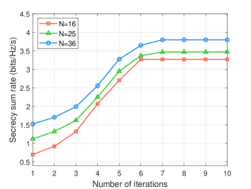
Figure 4: Convergence process: secrecy sum-rate versus number of iterations under different TRIS elements (${\varepsilon_{k}}=\sqrt{0.01},{\varepsilon_{m,n}}=0.1\sqrt{\kappa_{v}},P_{t}=1{\rm mW}$).

Secondly, we illustrate the secrecy spectral efficiency (SSE) varies with the maximum power of each transmissive element. As shown in Fig. 5, the SSE of the system increases as the maximum power of each TRIS element increases. Moreover, the SSE of the proposed architecture is second only to the traditional transceiver due to the fact that TMA constrains the rows of the ${\bf{W}}\left[l\right]$ and actually consumes less energy.

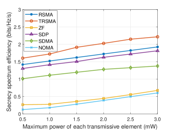
Figure 5: SSE varies with the maximum power of each transmissive element (${\varepsilon_{k}}=\sqrt{0.01},{\varepsilon_{m,n}}=0.1\sqrt{\kappa_{v}},N=16$).

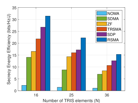
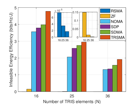
(a) SEE	(b) IEE

Figure 6: SEE and IEE varies with the number of TRIS element (${\varepsilon_{k}}=\sqrt{0.01},{\varepsilon_{m,n}}=0.1\sqrt{\kappa_{v}},P_{t}=1{\rm mW}$).

However, the SEE of the proposed scheme outperforms all the benchmarks as shown in Fig. 6 (a), which confirms the superiority of the TRIS transceiver in terms of SEE, as well as the 44% improvement in SEE compared to the traditional transceiver. And according to Fig. 6 (b), the infeasible energy efficiency (IEE) of the proposed scheme outperforms all the benchmark schemes and decreases with the increase in the number of TRIS elements, confirming the effectiveness of increasing the number of TRIS elements in reducing eavesdropping by IUs. In addition, SEE decreases as the number of TRIS elements increases, which is due to the increase in power consumption with the increase in TRIS elements, but the enhancement for the secrecy rate is minor.

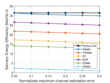
Figure 7: SEE varies with the normalized channel estimation error $\tau_{m}^{2}$ (${\varepsilon_{k}}=\sqrt{0.01},P_{t}=1{\rm mW},N=16$).

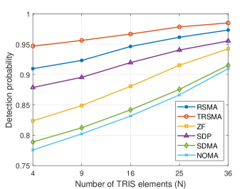
Figure 8: The detection probability of IU varies with the number of TRIS elements (${\varepsilon_{m,n}}=0.1\sqrt{\kappa_{v}},P_{t}=1{\rm mW}$).

Subsequently, in order to explore the effect of channel estimation error on the system’s SEE, it is demonstrated in Fig. 7. It can be seen that compared to perfect CSI, the SEE of the proposed scheme decreases as the channel error increases, has a 5% performance loss, but outperforms other schemes.

Next, we compare the changes in the detection probability of IU with the increase in the number of TRIS elements for each scheme as shown in Fig. 8. It can be seen that the IU detection probability of the proposed scheme is above 90% and higher than that of the baseline schemes except for the traditional transceivers, which is due to the fact that the traditional transceivers receive with multiple antennas while the TRIS transceivers receive with a single antenna. Moreover, the detection probability increases with the increase in the number of TRIS elements, which provides a guideline for designing a secure ISAC network.

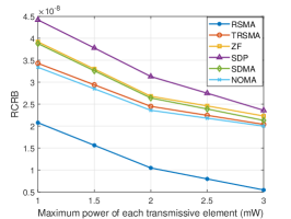
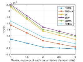
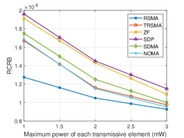
(a) $d$ RCRB	(b) $\theta$ RCRB	(c) $\phi$ RCRB

Figure 9: RCRB varies with the maximum power of each transmissive element ($P_{t}=1{\rm mW},N=16$).

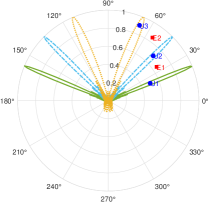
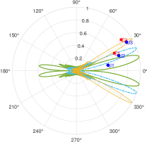
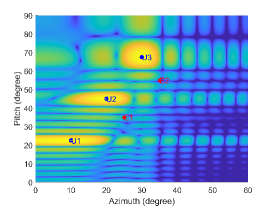
(a) Pitch	(b) Azimuth	(c) Beampattern

Figure 10: Beam scanning and beampattern ($P_{t}=1{\rm mW},N=36$).

Then, in order to compare the impact of each scheme on the perceived accuracy, we use root Cramér-Rao boundary (RCRB) as a criterion. From Fig. 9, the results show that RSMA outperforms the other schemes in terms of RCRB for distance, azimuth, and pitch, indicating that RSMA has a better ability to manage interference and adapt to radar sensing.

Next, in order to visualize the beampatterns, we show in Fig. 10 the beam scanning for timeslots 2, 3, and 4 as well as the beampattern. It is obvious that the beam of the proposed architecture in this paper can well cover the LUs, who are in the peak position of the beampattern, and the IUs are in a region of low beam energy.

Finally, in order to visualize the resource allocation throughout the service process, it is presented in Figure 11. It can be seen that most of the system’s power is allocated to timeslots 2, 3, and 4, and that the timeslots have the longest duration, matching the beam scanning results.

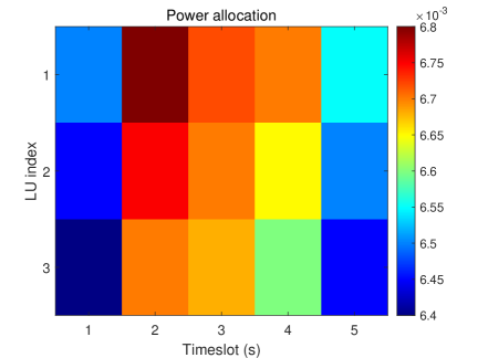
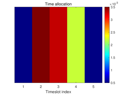
(a) Power allocation	(b) Timeslot duration allocation

Figure 11: Resource allocation ($P_{t}=1{\rm mW},N=36$).

VI Conclusions

In this paper, we propose a robust and secure ISAC architecture based on time-division. To facilitate the integration of sensing and communication, we deploy a novel TRIS transceiver framework and innovatively exploits the common stream of RSMA as both useful signals and AN to address the problem of IU eavesdropping and interference. Based on the architectural setup, we consider the problem of secure communication and potential IUs detection under conditions of imperfect CSI and networks serving multiple LUs with the presence of multiple IUs and give theoretical upper bounds on the error of IU channels. Also, to improve the security of the system, we consider the system outage. Based on these settings, we propose a joint robust and secure communication and sensing design algorithm. Numerical simulations verify the effectiveness of the proposed architecture and its advantages over other schemes. In addition, design guidelines are provided for future secure ISAC networks, i.e., increasing the number of TRIS elements, adopting RSMA, and adopting multi-timeslot beam scanning will result in better sensing and secure communication performance enhancement.

References

- [1] J. Zhang, T. Q. Duong, R. Woods, and A. Marshall, “Securing wireless communications of the Internet of things from the physical layer, an overview,” Entropy, vol. 19, no. 8, Aug. 2017. [Online]. Available: https://www.mdpi.com/1099-4300/19/8/420
- [2] P. Angueira, I. Val, J. Montalban, O. Seijo, E. Iradier, P. S. Fontaneda, L. Fanari, and A. Arriola, “A survey of physical layer techniques for secure wireless communications in industry,” IEEE Commun. Surv. Tutor., vol. 24, no. 2, pp. 810–838, Feb. 2022.
- [3] M. H. Khoshafa, O. Maraqa, J. M. Moualeu, S. Aboagye, T. M. Ngatched, M. H. Ahmed, Y. Gadallah, and M. Di Renzo, “RIS-assisted physical layer security in emerging RF and optical wireless communication systems: A comprehensive survey,” 2024. [Online]. Available: arXiv.2403.10412
- [4] H. V. Poor and R. F. Schaefer, “Wireless physical layer security,” Proc. Natl. Acad. Sci., vol. 114, no. 1, pp. 19–26, Dec. 2017.
- [5] A. Chorti, A. N. Barreto, S. Köpsell, M. Zoli, M. Chafii, P. Sehier, G. Fettweis, and H. V. Poor, “Context-aware security for 6G wireless: The role of physical layer security,” IEEE Commun. Mag., vol. 6, no. 1, pp. 102–108, Mar. 2022.
- [6] W. Khalid, M. A. U. Rehman, T. Van Chien, Z. Kaleem, H. Lee, and H. Yu, “Reconfigurable intelligent surface for physical layer security in 6G-IoT: Designs, issues, and advances,” IEEE Internet Things J., vol. 11, no. 2, pp. 3599–3613, Jul. 2024.
- [7] H. Alakoca, M. Namdar, S. Aldirmaz-Colak, M. Basaran, A. Basgumus, L. Durak-Ata, and H. Yanikomeroglu, “Metasurface manipulation attacks: Potential security threats of RIS-aided 6G communications,” IEEE Commun. Mag., vol. 61, no. 1, pp. 24–30, Nov. 2023.
- [8] X. Yuan, S. Hu, W. Ni, X. Wang, and A. Jamalipour, “Empowering reconfigurable intelligent surfaces with artificial intelligence to secure air-to-ground Internet-of-things,” IEEE Internet of Things Mag., vol. 7, no. 2, pp. 14–21, Mar. 2024.
- [9] Z. Li, Q. Lin, Y.-C. Wu, D. W. K. Ng, and A. Nallanathan, “Enhancing physical layer security with RIS under multi-antenna eavesdroppers and spatially correlated channel uncertainties,” IEEE Trans. Commun., vol. 72, no. 3, pp. 1532–1547, Nov. 2024.
- [10] D.-T. Do, A.-T. Le, N.-D. X. Ha, and N.-N. Dao, “Physical layer security for Internet of things via reconfigurable intelligent surface,” Future Gener. Comput. Syst., vol. 126, pp. 330–339, Jan. 2022. [Online]. Available: https://www.sciencedirect.com/science/article/pii/S0167739X21003204
- [11] H. Niu, Z. Lin, Z. Chu, Z. Zhu, P. Xiao, H. X. Nguyen, I. Lee, and N. Al-Dhahir, “Joint beamforming design for secure RIS-assisted IoT networks,” IEEE Internet Things J., vol. 10, no. 2, pp. 1628–1641, Sep. 2023.
- [12] Y. Sun, K. An, Y. Zhu, G. Zheng, K.-K. Wong, S. Chatzinotas, H. Yin, and P. Liu, “RIS-assisted robust hybrid beamforming against simultaneous jamming and eavesdropping attacks,” IEEE Trans. Wireless Commun., vol. 21, no. 11, pp. 9212–9231, May 2022.
- [13] L. Chai, L. Bai, T. Bai, J. Shi, and A. Nallanathan, “Secure RIS-aided MISO-NOMA system design in the presence of active eavesdropping,” IEEE Internet of Things J., vol. 10, no. 22, pp. 19 479–19 494, Apr. 2023.
- [14] M. Hua, Q. Wu, W. Chen, O. A. Dobre, and A. L. Swindlehurst, “Secure intelligent reflecting surface-aided integrated sensing and communication,” IEEE Trans. Wireless Commun., vol. 23, no. 1, pp. 575–591, Jan 2024.
- [15] N. Su, F. Liu, C. Masouros, and A. Al Hilli, Security and Privacy in ISAC Systems. Singapore: Springer Nature Singapore, 2023, pp. 477–506. [Online]. Available: https://doi.org/10.1007/978-981-99-2501-8_17
- [16] Z. Wei, F. Liu, C. Masouros, N. Su, and A. P. Petropulu, “Toward multi-functional 6G wireless networks: Integrating sensing, communication, and security,” IEEE Commun. Mag., vol. 60, no. 4, pp. 65–71, Apr. 2022.
- [17] D. H. Tashman and W. Hamouda, “An overview and future directions on physical-layer security for cognitive radio networks,” IEEE Netw., vol. 35, no. 3, pp. 205–211, Oct. 2021.
- [18] Z. Zhang, W. Chen, Q. Wu, Z. Li, X. Zhu, and J. Yuan, “Intelligent omni surfaces assisted integrated multi-target sensing and multi-user mimo communications,” IEEE Trans. Commun., pp. 1–1, Mar. 2024.
- [19] Z. Zhang, W. Chen, Q. Wu, Z. Li, X. Zhu, J. Chen, and N. Cheng, “Multiple intelligent reflecting surfaces collaborative wireless localization system,” 2024. [Online]. Available: arxiv.2406.09846
- [20] Z. Ren, L. Qiu, J. Xu, and D. W. K. Ng, “Robust transmit beamforming for secure integrated sensing and communication,” IEEE Trans. Commun., vol. 71, no. 9, pp. 5549–5564, Jun. 2023.
- [21] N. Su, F. Liu, and C. Masouros, “Sensing-assisted eavesdropper estimation: An ISAC breakthrough in physical layer security,” IEEE Trans. Wireless Commun., vol. 23, no. 4, pp. 3162–3174, Aug. 2024.
- [22] H. Jia, X. Li, and L. Ma, “Physical layer security optimization with Cramér-Rao bound metric in ISAC systems under sensing-specific imperfect CSI model,” IEEE Trans. Veh. Technol., vol. 73, no. 5, pp. 6980–6992, May 2024.
- [23] Y. Mao, O. Dizdar, B. Clerckx, R. Schober, P. Popovski, and H. V. Poor, “Rate-splitting multiple access: Fundamentals, survey, and future research trends,” IEEE Commun. Surv. Tutor., vol. 24, no. 4, pp. 2073–2126, Jul. 2022.
- [24] A. Mishra, Y. Mao, O. Dizdar, and B. Clerckx, “Rate-splitting multiple access for 6G-part I: Principles, applications and future works,” IEEE Commun. Lett., vol. 26, no. 10, pp. 2232–2236, Jul. 2022.
- [25] Y. Mao, B. Clerckx, and V. O. Li, “Energy efficiency of rate-splitting multiple access, and performance benefits over SDMA and NOMA,” in Int. Symp. Wireless Commun. Syst., Lisbon, Portugal, Oct. 2018, pp. 1–5.
- [26] H. Xia, Y. Mao, X. Zhou, B. Clerckx, S. Han, and C. Li, “Weighted sum-rate maximization for rate-splitting multiple access based multi-antenna broadcast channel with confidential messages,” 2023. [Online]. Available: arXiv.2202.07328
- [27] A. Salem, C. Masouros, and B. Clerckx, “Secure rate splitting multiple access: How much of the split signal to reveal?” IEEE Trans. Wireless Commun., vol. 22, no. 6, pp. 4173–4187, Dec. 2023.
- [28] Z. Liu, W. Chen, Q. Wu, J. Yuan, S. Zhang, Z. Li, and J. Li, “Rate-splitting multiple access for transmissive reconfigurable intelligent surface transceiver empowered ISAC systems,” IEEE Internet of Things J., pp. 1–1, May 2024.
- [29] Z. Liu, W. Chen, Z. Li, J. Yuan, Q. Wu, and K. Wang, “Transmissive reconfigurable intelligent surface transmitter empowered cognitive RSMA networks,” IEEE Commun. Lett., vol. 27, no. 7, pp. 1829–1833, May 2023.
- [30] C. He, “Theory and application research for time modulated array,” Ph.D. dissertation, Shanghai Jiao Tong University, 2015.
- [31] H. Guo and V. K. N. Lau, “Uplink cascaded channel estimation for intelligent reflecting surface assisted multiuser MISO systems,” IEEE Trans. Signal Process., vol. 70, pp. 3964–3977, Jul. 2022.
- [32] F. Dong, F. Liu, Y. Cui, W. Wang, K. Han, and Z. Wang, “Sensing as a service in 6G perceptive networks: A unified framework for ISAC resource allocation,” IEEE Trans. Wireless Commun., vol. 22, no. 5, pp. 3522–3536, Nov. 2023.
- [33] D. Fuhrmann and G. San Antonio, “Transmit beamforming for MIMO radar systems using partial signal correlation,” in Conf. Rec. Asilomar Conf. Signals Syst. Comput., vol. 1, Pacific Grove, CA, United states, 2004, pp. 295–299 Vol.1.
- [34] I. Bechar, “A Bernstein-type inequality for stochastic processes of quadratic forms of Gaussian variables,” arXiv:0909.3595, 2009.
- [35] A. Bazzi and M. Chafii, “On outage-based beamforming design for dual-functional radar-communication 6G systems,” IEEE Trans. Wireless Commun., vol. 22, no. 8, pp. 5598–5612, Jan. 2023.
- [36] S. Boyd and L. Vandenberghe, Convex optimization. Cambridge university press, 2004.
- [37] Y. Li, M. Jiang, Q. Zhang, and J. Qin, “Joint beamforming design in multi-cluster MISO NOMA reconfigurable intelligent surface-aided downlink communication networks,” IEEE Trans. Commun., vol. 69, no. 1, pp. 664–674, Oct. 2021.
- [38] K.-Y. Wang, A. M.-C. So, T.-H. Chang, W.-K. Ma, and C.-Y. Chi, “Outage constrained robust transmit optimization for multiuser MISO downlinks: Tractable approximations by conic optimization,” IEEE Trans. Signal Process., vol. 62, no. 21, pp. 5690–5705, Sep. 2014.
- [39] M. Grant and S. B. (2014), “CVX: MATLAB software for disciplined convex programming, Version 2.1.” [Online]. Available: http://cvxr.com/cvx/
- [40] A. Ben-Tal and A. Nemirovski, “Lectures on modern convex optimization: Analysis, algorithms, and engineering applications / A. Ben-Tal, A. Nemirovski.”