F2PAD: A General Optimization Framework for Feature-Level to Pixel-Level Anomaly Detection

Abstract

Image-based inspection systems have been widely deployed in manufacturing production lines. Due to the scarcity of defective samples, unsupervised anomaly detection that only leverages normal samples during training to detect various defects is popular. Existing feature-based methods, utilizing deep features from pretrained neural networks, show their impressive performance in anomaly localization and the low demand for the sample size for training. However, the detected anomalous regions of these methods always exhibit inaccurate boundaries, which impedes the downstream tasks. This deficiency is caused: (i) The decreased resolution of high-level features compared with the original image, and (ii) The mixture of adjacent normal and anomalous pixels during feature extraction. To address them, we propose a novel unified optimization framework (F2PAD) that leverages the Feature-level information to guide the optimization process for Pixel-level Anomaly Detection in the inference stage. The proposed framework is universal and can enhance various feature-based methods with limited assumptions. Case studies are provided to demonstrate the effectiveness of our strategy, particularly when applied to three popular backbone methods: PaDiM, CFLOW-AD, and PatchCore. Our source code and data will be available upon acceptance.

Note to Practitioners

Visual quality inspection systems are popular in modern industries for defect detection on the surface of manufacturing products. Since the defects are rare during production, it is suitable to collect the normal samples as the training dataset and then detect unseen defects at testing. The feature-based methods are popular, which can localize the anomaly well and handle small-batch production, i.e., only a few normal samples are collected for training. However, these methods cannot guarantee precise anomaly boundaries, which is undesired for anomaly characterization and further diagnosis. This paper analyzes the two issues that correspond to the above problem and proposes a novel general optimization framework to achieve precise anomaly boundary segmentation at the pixel level. The proposed method can be applied to enhance a wide range of existing feature-based methods, including the well-known PaDiM, CFlow, and PatchCore, which is demonstrated by the extensive case studies. By implementing our method, practitioners can obtain more accurate anomaly information, benefiting other downstream tasks and objectives.

I Introduction

Automated visual inspection of products by deploying cost-efficient image sensors has become a critical concern in industrial applications in recent years, ranging from microscopic fractions and crack detection on electrical commutators [1] to fabric defect detection on textiles [2]. In realistic production lines, defective products are always scarce. Moreover, all possible types of defects that occurred during production are impossible to know beforehand [3, 4]. In this scenario, only utilizing normal (non-defective) samples to train modern machine learning models for defect detection becomes essential. Therefore, unsupervised anomaly detection has become a mainstream setting in practical applications.

Besides determining whether a sample is anomalous or not, it is also essential to precisely localize and segment the defective regions due to the following reasons: (i) It enables the characterization of surface defects, such as shape, size, and orientation [5], which contributes to the evaluation of product quality [6]. (ii) It benefits the subsequent defect classification and recognition [7], as the models could focus more on the discriminative regions. An example is provided in Fig. 1, where the target defective region is masked as white in the ground truth (GT).

Current unsupervised image anomaly detection methods can be mainly categorized into two groups [8]: (1) Image reconstruction-based methods. These methods deploy various neural network architectures for the reconstruction of an input image, such as Autoencoders (AE) [9, 10] and Generative Adversarial Networks (GAN) [11]. Therefore, the per-pixel comparison between the input and reconstructed images can localize anomaly. (2) Feature-based methods. These methods mainly rely on deep features extracted from neural networks pretrained on large-scale image databases like ImageNet[12]. The collected features of normal samples can be modeled in different ways. Then, associated distance metrics are defined to describe the normality of test features [13, 14, 15, 16]. Section II provides a more detailed literature review.

To guarantee the high-fidelity reconstruction of normal regions at the pixel level, image reconstruction-based methods require sufficient normal samples. In contrast, owing to the great expressiveness of deep features even for unseen manufacturing parts in industries, feature-based methods have less demand for the sample size of the training dataset. However, though the existence and location of anomalies can be identified well by the feature-based methods, the boundaries of detected anomalies are always inaccurate [17, 3, 18]. To illustrate this point, the first row of Fig. 1 visualizes the unsatisfactory anomaly segmentation results of PatchCore [19], CFLOW-AD [16], and PaDiM [13] with relatively low evaluation metrics.

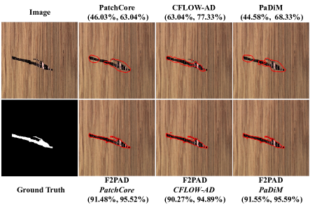
Figure 1: An example of F2PAD’s anomaly detection results. Top row: Test image and the anomaly detection results (Intersection over Union (IOU), DICE coefficient) of three popular feature-based methods, i.e., PatchCore [19], CFLOW-AD [16], and PaDiM [13]. Bottom row: Ground truth and the results of F2PAD when applied to the above three methods. Our F2PAD significantly enhances the original PatchCore, PaDiM, and CFLOW-AD methods with higher anomaly segmentation accuracy, demonstrated by the improved IOU and DICE metrics.

To explain the above common deficiency in feature-based methods, we summarize the two issues as follows:

• Issue 1: Decreased resolution of the feature map. The popular choices for pretrained networks are Convolutional Neural Networks (CNN). With the multi-scale pyramid pooling layers, the feature map constructed from a deeper layer has a smaller resolution than the previous layers. For instance, in [13], the resolution of an input image is $224\mathrm{(height)}\times 224\mathrm{(width)}$, while the sizes of feature maps extracted from the $1\textrm{st}$ and $3\textrm{th}$ layers of the ResNet18 [20] are $56\times 56$ and $14\times 14$, respectively. In addition, the patch representation, which is spatially downsampled from the original image, is adopted in Vision Transformers (ViTs) [21] and the self-supervised feature learning [22]. Since anomaly detection is conducted at the feature (patch) level, per-pixel accuracy cannot be achieved.

• Issue 2: Mixture of adjacent normal and anomalous pixels. To extract a specific feature, all adjacent pixels falling within its receptive field (or the associated patch) are considered. Consequently, features near anomaly boundaries aggregate information from both normal and anomalous pixels. These features are often confusing and difficult to discriminate accurately, resulting in unclear anomaly segmentation.

This paper aims to tackle the above two issues concurrently, enabling accurate anomaly segmentation in feature-based methods. To achieve this, we propose a novel optimization framework for Feature-level to Pixel-level Anomaly Detection (F2PAD). Specifically, we can decompose an arbitrary input image into two unknown parts, i.e., a non-defective image plus an anomalous part, which have the same resolutions as the original image. Then, an optimization model is proposed, which encourages the non-defective image to produce normal features. In this way, the anomaly is directly indicated by the estimated anomalous part, which remains the original resolution. Furthermore, feature extraction is performed solely on the estimated non-defective image without the mixture of different types of pixels. The above properties directly avoid the aforementioned issues. To end up, our main contributions are summarized as follows:

• We propose a general optimization framework to enhance a variety of feature-based methods for precise pixel-level anomaly segmentation in industrial images, with examples of PatchCore [19], CFLOW-AD [16], and PaDiM [13].

• We propose a novel penalized regression model that concurrently estimates the non-defective image and anomalous part. The loss function originates from an established feature-based approach, and we incorporate two regularization terms: a sparsity-inducing penalty for identifying anomalies and a pixel prior term to enhance non-defective image recovery.

• We design an optimization algorithm for the above regression problem with a novel local gradient-sharing mechanism, which empirically shows better optimization results.

The remainder of this paper is organized as follows. Section II reviews the literature about industrial image anomaly detection. Section II discusses the formulation of our proposed framework. Then, case studies including various categories of realistic products are provided in Section IV to validate our methodology. Finally, Section V summarizes this paper.

II Related Work

This section reviews the following two categories of industrial image anomaly detection methods in the literature.

II-A Image Reconstruction-Based Methods

Reconstruction-based image anomaly detection methods aim to reconstruct the normal samples accurately during training, assuming imperfect reconstruction of defective regions for an anomalous image during inference. The pixel differences between the input and reconstructed images can be directly transformed into anomaly scores and further thresholded as a binary anomaly mask. Therefore, the key research goal is to pursue a more accurate reconstruction. Autoencoder (AE) is the most prevalent architecture for image reconstruction [23, 24, 25]. In AEs, a common choice of the backbone network is CNN. Vision transformers were introduced in [26, 27] to capture more global structural information. Besides the AEs, GANs [11, 28] and diffusion models [29, 30] are also popular choices.

Instead of focusing on the architecture of the reconstruction network, there are various strategies to improve the reconstruction accuracy. For example, the structure similarity index measure (SSIM) was introduced in [9] to incorporate the perceptual difference of anomaly. Additionally, to address the deterioration of image reconstruction caused by anomalies, [31, 32] enforced the reconstructed image on the learned manifold. Alternatively, [33] adopted a self-supervised learning way by generating synthetic anomalies to avoid reconstructing undesired anomalies.

Nevertheless, sufficient normal samples are necessary for pixel-wise reconstruction in the image reconstruction-based methods [18].

II-B Feature-Based Methods

Utilizing features with higher-level information avoids the necessity of per-pixel reconstruction. Generally, feature-based methods consist of two subsequent steps [3]: (i) Feature extraction. It can be achieved by employing various CNNs and ViTs pretrained on large-size image databases or can be learned in a self-supervised way with patch representation [22]. (ii) The modeling of normal features. Most methods in the literature focus on this step, which will be comprehensively reviewed in this subsection. After this step, anomaly scores are assigned to individual features and then simply interpolated to yield pixel-level results.

PaDiM [13] adopted the multivariate Gaussian distributions to model the normal features. To allow more complicated probabilistic distributions, DifferNet [15] adopted a neural network, i.e., normalizing flow, to estimate the density of features. Furthermore, CFLOW-AD [16] improved the DifferNet by modeling the conditional probabilities of features on their locations. Similarly, a 2D normalizing flow was proposed in [34] to retain the spatial relationship between features. The memory bank-based method that collects all normal features was first proposed in [35], while the average distance of a test feature to its k-nearest neighbors was regarded as the anomaly score. To improve the inference speed, the coreset technique was adopted in PatchCore[19] by greedily selecting the farthest features to construct a reduced memory bank. Similarly, [36] proposed a gradient preference strategy to determine the most significant features for anomaly detection. In addition, the deep support vector domain description (SVDD) was adopted in [22, 37] to map normal image patches within compact spheres. Teacher-student networks were also popular in literature [38], which effectively transfer normal features from the teacher network to the student model but fail for anomalous features.

One issue of the above methods is the decreased resolution of the feature map, as stated in Issue 1. To tackle it, the work [17] learned dense features in the image size by using the multipooling and unwarping strategy in [39]. However, it is only applicable to local patch descriptions by CNNs. Furthermore, the anomaly scores were defined as the gradients of loss function w.r.t the input image in [38]. Therefore, feature-level scores are no longer required. However, this strategy may not achieve satisfactory results for general methods in practice [31]. Finally, the work [40] proposed a refinement network to refine the initial anomaly map, utilizing the input image as additional channels. However, this method requires more samples to train the refinement network. In addition, the mixture of normal and anomalous pixels described in Issue 2 remains unsolved in the above methods [17, 38, 40].

In summary, current literature lacks a general framework to deal with Issues 1&2 discussed in Section I simultaneously in feature-based methods. Our proposed F2PAD can achieve the above goal with limited assumptions, which will be discussed in detail in the following Section III.

III Methodology

We first clarify our objective and formulate the problem as a penalized regression problem by our F2PAD in Section III-A. Then, Sections III-B and III-C show the details about the loss functions and regularization terms respectively. In addition, we propose a novel optimization algorithm in Section III-D. Finally, the implementation details are present in Section III-E.

III-A Overview

III-A1 Preliminary

Given an input RGB image $\mathbf{x}\in\mathbb{R}^{h\times w\times 3}$ with height $h$ and width $w$, our goal is to obtain a binary anomaly mask $\mathbf{m}\in\{0,1\}^{h\times w}$, where $\mathbf{m}_{i,j}=1$ indicates an anomalous pixel in row $i$ and column $j$, and normal otherwise.

For the feature-based methods, a feature extractor $\mathbf{\phi}_{k}$ is utilized to extract the feature map $\mathbf{f}_{k}=\mathbf{\phi}_{k}(\mathbf{x})\in\mathbb{R}^{h_{k}\times w_{k}\times c_{k}}$ in layer $k$, where $h_{k}$, $w_{k}$, and $c_{k}$ are height, width, and the number of feature channels, respectively. Then, anomaly score $s_{k,i,j}\in\mathbb{R}$ assigned to the feature $\mathbf{f}_{k,i,j}\in\mathbb{R}^{c_{k}}$ is given by the scoring function $s_{k,i,j}=\mathbf{\psi}_{k}(\mathbf{f}_{k,i,j})$. Notably, Issue 1 in Section I indicates that the resolution $(h_{k},w_{k})$ is always smaller than $(h,w)$. $\mathbf{\phi}_{k}$ is learned during training and fixed for inference. We use $\nabla$ to denote the gradient.

III-A2 Assumptions

To allow the formulation of our F2PAD, we make the following two assumptions:

• The (approximated) gradients of feature extractor $\mathbf{\phi}_{k}$ and scoring function $\mathbf{\psi}_{k}$ exist. For example, $\mathbf{\phi}_{k}$ defined by neural networks in almost all existing works, e.g., CNNs and ViTs, meet the above requirement that enables backpropagation (BP). Furthermore, $\mathbf{\psi}_{k}$ is always defined as probabilistic metrics, e.g., the log-likelihood, or distance metrics, such as the $l_{2}$ and Mahalanobis distances. Modern deep learning libraries can automatically compute the gradients (approximately) of common mathematical operations, such as the $\mathrm{autograd}$ module in PyTorch [41]. Therefore, a variety of methods support this assumption.

• The anomalies are locally distributed. The common surface defects, including holes, dents, cracks, and scratches, show the above property. In addition, this assumption is also adopted in various anomaly detection works [42, 43, 44, 45].

III-A3 Overall Framework

Motivated by the decomposition ideas [31, 43], we assume an additive model as follows:

$$\mathbf{x}=\mathbf{n}+\mathbf{a},$$ (1)

where $\mathbf{n},\mathbf{a}\in\mathbb{R}^{h\times w\times 3}$ are the non-defective image and the anomalous part respectively. The relationship between the mask $\mathbf{m}$ and $\mathbf{a}$ is that

$$\mathbf{m}_{i,j}=1\ \mathrm{iff}\ \mathbf{a}_{i,j}\neq 0.$$ (2)

Then, the anomaly segmentation problem in this paper is to estimate $\mathbf{n}$ and $\mathbf{a}$ in a unified model. Specifically, the separation of $\mathbf{n}$ and $\mathbf{a}$ in Eq. (1) indicates that there is no anomaly in the non-defective image $\mathbf{n}$. Then, we can define a loss function $l_{n}(\mathbf{n})$ to encourage small anomaly scores $\{s_{k,i,j}\}$ for the features extracted from $\mathbf{n}$. Concurrently, a sparsity-inducing penalty $l_{a}(\mathbf{a})$ is introduced to promote the locality of anomalies, as assumed in Section III-A2. Since $l_{n}(\mathbf{n})$ is related to high-level features, another regularization term, i.e., the pixel prior $l_{p}(\mathbf{n})$, is necessary to enhance the recovery of $\mathbf{n}$. Finally, the penalized regression problem with objective function $F(\mathbf{n},\mathbf{a})$ is formulated as follows:

$$\mathop{\min}\limits_{\mathbf{n},\mathbf{a},\mathbf{x}=\mathbf{n}+\mathbf{a}}F(\mathbf{n},\mathbf{a})=l_{n}(\mathbf{n})+\alpha l_{p}(\mathbf{n})+\beta l_{a}(\mathbf{a}).$$ (3)

III-A4 Discussion

There are the following properties in the problem (3) that contribute to the goal of this paper:

• For Issue 1, $\mathbf{a}$ remains the same resolution as $\mathbf{x}$, indicating that the pixel-level detection can be directly given by solving the problem (3).

• For Issue 2, feature extraction is solely performed on $\mathbf{n}$, as shown in loss $l_{n}(\mathbf{n})$, which is not influenced by the appeared anomalies.

• The first assumption in Section III-A2 means that the problem (3) is practically solvable through gradient-based algorithms.

The following subsections will show more details about the problem (3).

III-B Loss Functions

This subsection shows three examples of loss functions $l_{n}(\mathbf{n})$ when applied to PatchCore [19], CFLOW-AD [16], and PaDiM [13], respectively.

III-B1 PatchCore

: Following [19], we concatenate all feature maps in different layers into a single one $\mathbf{f}\in\mathbb{R}^{h_{1}\times w_{1}\times c}$, with $c=\sum_{k}c_{k}$, remaining the same size as the largest feature map $\mathbf{f}_{1}$. Given the memory bank $\mathcal{M}$ with $|\mathcal{M}|$ normal features collected from the training dataset, the anomaly score $s_{i,j}$ of $\mathbf{f}_{i,j}$ is defined as the minimum distance to the memory bank:

$$s_{i,j}=\min_{\mathbf{f}_{m}\in\mathcal{M}}\|\mathbf{f}_{i,j}-\mathbf{f}_{m}\|^{2}_{2}.$$ (4)

We need to consider the whole $\mathcal{M}$ in Eq. (4), which heavily influences the computational speed. In practice, we can only consider a small candidate set $\mathcal{M}_{i,j}\in\mathcal{M},|\mathcal{M}_{i,j}|\ll|\mathcal{M}|$ for each $\mathbf{f}_{i,j}$ to approximate $s_{i,j}$ as

$$s^{\prime}_{i,j}=\min_{\mathbf{f}_{m}\in\mathcal{M}_{i,j}}\|\mathbf{f}_{i,j}-\mathbf{f}_{m}\|^{2}_{2}.$$ (5)

Based on Eq. (5), we can define the final loss as the summation of scores over all pixels, i.e., $l_{n}(\mathbf{n})=\sum_{i,j}s^{\prime}_{i,j}$.

To construct $\mathcal{M}_{i,j}$, we assume that we have an initial estimate of $\mathbf{n}$ in (3), denoted as $\mathbf{n}^{(0)}$, which subsequently provides an initial $\mathbf{f}_{i,j}^{(0)}$. Then, we define $\mathcal{M}_{i,j}$ as the $|\mathcal{M}_{i,j}|$ nearest features of $\mathbf{f}_{i,j}^{(0)}$ in $\mathcal{M}$. Therefore, if $\mathbf{f}_{i,j}^{(0)}$ is not far from the optimal value, Eq. (5) can approximate well Eq. (4). We will discuss how to access $\mathbf{n}^{(0)}$ in Section III-E1.

III-B2 CFLOW-AD

: In this method, to incorporate the positional information, the feature map $\mathbf{f}_{k}$ in layer $k$ is concatenated with $\mathbf{c}_{k}\in R^{h_{k}\times w_{k}\times 128}$, i.e., $\mathbf{f}_{k}=\mathbf{f}_{k}\oplus\mathbf{c}_{k}$. $\mathbf{c}_{k}$ is obtained by the position encoding with $\mathrm{sin}$ and $\mathrm{cos}$ harmonics [16]. Notably, $\mathbf{c}_{k}$ is irrelevant to $\mathbf{n}$.

The log-likelihood $\log p(\mathbf{f}_{k,i,j}|\mathbf{\theta}_{k})$ is modeled by a normalizing flow with parameters $\mathbf{\theta}_{k}$. To speed up the optimization, we apply the $\mathrm{LogSigmoid}$ operation to the log-likelihood to define the anomaly score as:

$$s_{k,i,j}=\log(\dfrac{p(\mathbf{f}_{k,i,j})}{(1+p(\mathbf{f}_{k,i,j})}).$$ (6)

Similar to PatchCore, we define $l_{n}(\mathbf{n})=\sum_{k,i,j}s_{k,i,j}$.

III-B3 PaDiM

: PaDiM follows the same procedure of feature concatenation as PatchCore. $\mathbf{f}_{i,j}$ follows a multivariate Gaussian distribution with mean $\mathbf{\mu}_{i,j}\in\mathbb{R}^{c}$ and covariance $\mathbf{\Lambda}_{i,j}\in\mathbb{R}^{c\times c}$. Then, the anomaly score $s_{i,j}$ is defined by the square of Mahalanobis distance [13] as follows:

$$s_{i,j}=(\mathbf{f}_{i,j}-\bm{\mu}_{i,j})^{T}\mathbf{\Lambda}_{i,j}^{-1}(\mathbf{f}_{i,j}-\bm{\mu}_{i,j}).$$ (7)

We have $l_{n}(\mathbf{n})=\sum_{i,j}s_{i,j}$.

III-B4 Discussion

Since the above methods adopt neural networks as feature extractor $\mathbf{\phi}_{k}$, we can easily access the gradients of $\mathbf{f}_{i,j}$ and $\mathbf{f}_{k,i,j}$ w.r.t. $\mathbf{n}$, i.e., $\nabla_{\mathbf{n}}\mathbf{f}_{i,j}$ and $\nabla_{\mathbf{n}}\mathbf{f}_{k,i,j}$ respectively. Moreover, Eqs. (5), (6), and (7) show that it is able to derive the gradients $\nabla_{\mathbf{f}_{i,j}}s_{i,j}$ and $\nabla_{\mathbf{f}_{k,i,j}}s_{k,i,j}$. Therefore, the first assumption in Section III-A2 is valid for the above three methods. Following the chain rule, we can acquire $\nabla_{\mathbf{n}}l_{n}(\mathbf{n})$.

III-C Regularization Terms

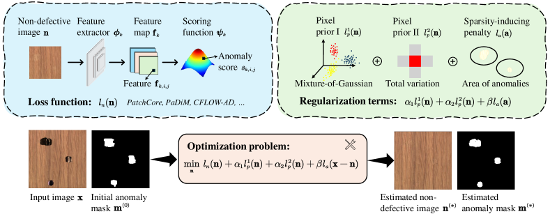
Figure 2: Schematic diagram of our F2PAD. We propose a novel optimization problem, which consists of the loss function $l_{n}(\mathbf{n})$ derived from feature-based methods, and three regularization terms $l_{p}^{1}(\mathbf{n})$, $l_{p}^{2}(\mathbf{n})$, and $l_{a}(\mathbf{a})$ as different roles. Given the input image $\mathbf{x}$ and initial anomaly mask $\mathbf{m}^{(0)}$ obtained by the original backbone methods (see Section III-E1), we can accurately estimate the non-defective image $\mathbf{n}^{(*)}$ with mask $\mathbf{m}^{(*)}$ by solving the proposed optimization problem.

This subsection illustrates the motivation and specific definitions of $l_{a}(\mathbf{a})$ and $l_{p}(\mathbf{n})$.

III-C1 $l_{a}(\mathbf{a})$

This term is used to promote local anomalies. From the definition of $\mathbf{a}$ in Eq. (1), the number of anomalous pixels is given by the $l_{0}$ norm $\sum_{i,j}\|\mathbf{a}_{i,j}\|_{0}$. However, the $l_{0}$-based problem is NP-hard and the gradient does not exist, making it hard to efficiently solve the problem (3). Although the $l_{1}$ norm is a common practice [32, 31] as the convex relaxation of $l_{0}$ norm, it suffers the issue of inaccurate estimation in anomaly detection [42]. To address it, this paper adopts the nonconvex LOG penalty [46, 42] for $l_{a}(\bm{a})$ as follows:

$$l_{a}(\mathbf{a})=\sum_{i,j}\log(\sqrt{\|\mathbf{a}_{i,j}\|^{2}_{2}+\epsilon}+\|\mathbf{a}_{i,j}\|_{2}),$$ (8)

where $\epsilon$ is a hyperparameter.

III-C2 $l_{p}(\mathbf{n})$

It is also important to accurately recover $\mathbf{n}$ in (3). However, the loss $l_{n}(\mathbf{n})$ is directly defined by the high-level information encoded by features, as discussed in Section III-B. This indicates that the low-level pixel values cannot be uniquely determined. Consequently, the estimation of $\mathbf{a}$ will be influenced, leading to inaccurate detection results. To tackle it, we introduce the following two types of pixel priors.

Since the training dataset is available, the pixel value of a test image is expected to fall within some known ranges. Formally, we can model the prior distribution of a pixel. An image may contain the background and the foreground object, while the object comprises several components associated with different colors. Therefore, we assume that the pixel $\mathbf{n}_{i,j}$ follows a mixture-of-Gaussian (MOG) distribution:

$$\begin{split}p(\mathbf{n}_{i,j})&=\sum_{q}r_{q}\cdot(2\pi)^{-3/2}|\mathbf{\Lambda}_{q}|^{-1/2}\\ \cdot&\exp(-\dfrac{(\mathbf{n}_{i,j}-\bm{\mu}_{q})^{T}\mathbf{\Lambda}_{q}^{-1}(\mathbf{n}_{i,j}-\bm{\mu}_{q})}{2}),\end{split}$$ (9)

where $r_{q}\in\mathbb{R}$, $\bm{\mu}_{q}\in\mathbb{R}^{3}$, and $\mathbf{\Lambda}_{q}\in\mathbb{R}^{3\times 3}$ is the prior, mean, and covariance of the $q\mathrm{th}$ component of MOG, respectively. We adopt the algorithm [47] to estimate $r_{q}$, $\bm{\mu}_{q}$, and $\mathbf{\Lambda}_{q}$ by randomly sampling sufficient pixels from the training dataset.

To construct $l_{p}(\mathbf{n})$, we do not assign the priors $\{r_{q}\}$. Instead, we assume the equal probability of each component of MOG. This reduces the bias of converging to the most frequently occurring pixels in the training set. Combining Eq. (9) and similar to the Mahalabobis distance in Eq. (7), we can define a specification of $l_{p}(\mathbf{n})$ as:

$$l_{p}^{1}(\mathbf{n})=\sum_{i,j}\min_{q}(\mathbf{n}_{i,j}-\bm{\mu}_{q})^{T}\mathbf{\Lambda}_{q}^{-1}(\mathbf{n}_{i,j}-\bm{\mu}_{q}),$$ (10)

which focuses on the most likely component.

Furthermore, Eq. (10) is defined by individual pixels, ignoring the spatial relationship between neighboring pixels. Since the images of industrial objects always exhibit piece-wise smoothness, we consider the total variation (TV) regularization as another term $l_{p}^{2}(\mathbf{n})$ to promote the piece-wise smoothness [48]:

$$l_{p}^{2}(\mathbf{n})=\sum_{i,j}\|\mathbf{n}_{i+1,j}-\mathbf{n}_{i,j}\|_{2}+\|\mathbf{n}_{i,j+1}-\mathbf{n}_{i,j}\|_{2}.$$ (11)

With Eqs. (10) and (11), we can substitute $\mathbf{a}=\mathbf{x}-\mathbf{n}$ and rewrite the problem (3) as:

$$\min_{\mathbf{n}}F(\mathbf{n})=l_{n}(\mathbf{n})+\alpha_{1}l_{p}^{1}(\mathbf{n})+\alpha_{2}l_{p}^{2}(\mathbf{n})+\beta l_{a}(\mathbf{x}-\mathbf{n}),$$ (12)

where $\alpha_{1}$ and $\alpha_{2}$ are the corresponding tuning parameters of $l_{p}^{1}(\mathbf{n})$ defined in Eq. (10)$l_{p}^{2}(\mathbf{n})$ defined in Eq. (11), respectively. The schematic diagram of our proposed F2PAD is illustrated in Fig. 2.

III-D Optimization Algorithm

According to our discussions in Section III-B and Eqs. (8), (10), and (11), it is possible to use the gradient-based algorithm to solve the problem (12). However, due to the complicated structure of (12) built on deep neural networks, the solutions of some pixels obtained by popular algorithms may be poor. The gradients will diminish at these pixels and thus early stop. To deal with this challenge, we propose a novel local gradient-sharing mechanism, as illustrated in Fig. 3.

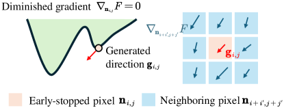
Figure 3: Motivation of our proposed local gradient-sharing mechanism.

The key idea is that for a pixel, it is possible to use its spatially neighboring pixels’ gradients to construct a feasible descending direction. In this way, the early-stopped pixels can still be pushed to escape the local minima. To achieve this, we can update the pixel $\mathbf{n}_{i,j}$ along the direction $\mathbf{g}_{i,j}\in\mathbb{R}^{3}$:

$$\mathbf{g}_{i,j}=\sum_{i^{\prime},j^{\prime}}w_{i^{\prime},j^{\prime}}\cdot\nabla_{\mathbf{n}_{i+i^{\prime},j+j^{\prime}}}F(\mathbf{n}),$$ (13)

where $i^{\prime},j^{\prime}\in[-k_{s},k_{s}]$ and $k_{s}$ indicates the neighborhood size. $\nabla_{\mathbf{n}_{i+i^{\prime},j+j^{\prime}}}F(\mathbf{n})$ is the gradient of the objective function $F(\mathbf{n})$ w.r.t. the neighboring pixel $\mathbf{n}_{i+i^{\prime},j+j^{\prime}}$ in Eq. (12). The weight $w_{i^{\prime},j^{\prime}}\in\mathbb{R}$ is defined as:

$$w_{i^{\prime},j^{\prime}}\propto\exp(-\dfrac{{i^{\prime}}^{2}+{j^{\prime}}^{2}}{\sigma_{0}})\exp(-\dfrac{\|\mathbf{x}_{i+i^{\prime},j+j^{\prime}}-\mathbf{x}_{i,j}\|_{2}^{2}}{\sigma_{1}}),$$ (14)

where the two terms measure the influence of neighboring pixels in terms of their spatial locations and colors with hyperparameters $\sigma_{0}$ and $\sigma_{1}$ respectively. Eq. (14) indicates that we assign larger weights to the more similar pixels. Finally, we normalize $\{w_{i^{\prime},j^{\prime}}\}$ such that $\sum_{i^{\prime},j^{\prime}}w_{i^{\prime},j^{\prime}}=1$.

In addition, our empirical results show that as $\mathbf{a}_{i,j}\rightarrow 0$, the corresponding gradient is relatively small, requiring a large step size to guarantee significant updating. Therefore, we propose an adaptive step size $\bm{\gamma}_{i,j}\in\mathbb{R}^{3}$ for the pixel $\mathbf{n}_{i,j}$ as:

$$\bm{\gamma}_{i,j}=\gamma_{0}/|\mathbf{a}_{i,j}|=\gamma_{0}/|\mathbf{x}_{i,j}-\mathbf{n}_{i,j}|,$$ (15)

where $\gamma_{0}$ is a constant and $|\cdot|$ takes the absolute values. Notably, we calculate $\bm{\gamma}_{i,j}$ in each iteration during optimization.

Finally, based on the descending direction $\mathbf{g}_{i,j}$ in Eq. (13) and step size $\bm{\gamma}_{i,j}$ in Eq. (15), we update $\mathbf{n}_{i,j}$ following the rule in the adaptive Nesterov momentum algorithm (Adan) [49]. We will demonstrate the performance of our proposed algorithm compared to the standard Adan in Section IV-C3.

III-E Implementation

Algorithm 1 . The whole procedure of our F2PAD.

Input: $\alpha_{1}$, $\alpha_{2}$, $\beta$, $\gamma_{0}$, $\sigma_{0}$, $\sigma_{1}$, $l_{n}(\mathbf{n})$, $\epsilon$, $\{\bm{\mu}_{q},\bm{\mathbf{\Lambda}}_{q}\}$.
Initialize: $\mathbf{m}^{(0)}$.
Output: $\mathbf{m}^{(*)}$, and optional $\mathbf{n}^{(*)}$.

1:Obtain the initial $\mathbf{n}^{(0)}$ by $\mathbf{m}^{(0)}$, as discussed in Section III-E1.

2:Obtain a sub-region of $\mathbf{n}$ to be optimized and construct the associated $l_{n}(\mathbf{n})$, according to Section III-E2.

3:Calculate the weights $\{w_{i^{\prime},j^{\prime}}\}$ by Eq. (14).

4:repeat

5:   Compute the descending directions $\{\mathbf{g}_{i,j}\}$ by Eq. (13).

6:   Adjust the step sizes $\{\bm{\mathbf{\gamma}}_{i,j}\}$ by Eq. (15).

7:   Update $\mathbf{n}$ by following Adan with $\{\mathbf{g}_{i,j}\}$ and $\{\bm{\mathbf{\gamma}}_{i,j}\}$.

8:until Meet stopping criteria.

9:Obtain the final $\mathbf{m}^{(*)}$ by Eqs. (1) and (2).

10:Re-estimate the final $\mathbf{n}^{(*)}$ according to $\mathbf{m}^{(*)}$, as discussed in Section III-E3.

This subsection presents the initialization and acceleration of our proposed framework and further summarizes the entire procedure.

III-E1 Initialization

To solve the problem (12), it is required to obtain an initial solution $\mathbf{n}^{(0)}$. Fortunately, we can utilize the anomaly mask $\mathbf{m}^{(0)}$ obtained by the original procedure of backbone methods. Concretely, the task of obtaining $\mathbf{n}^{(0)}$ can be transformed into an image inpainting task, i.e., infer the missing pixels under the masked region of $\mathbf{m}^{(0)}$. This paper utilizes a pretrained masked autoencoder (MAE) [50] for inpainting. The MAE captures both local and global contextual relationships, capable of dealing with various sizes of missing regions. Notably, the MAE is expected to provide only a rough pixel-level reconstruction, sufficient for initialization. We will show the improvement of our final result by solving (12) compared to the initialization in Section IV-C1.

III-E2 Acceleration

To speed up our algorithm, we only optimize the region of $\mathbf{n}$ indicated as anomalous by $\mathbf{m}^{(0)}$. As $\mathbf{m}^{(0)}$ may not completely cover the ground truth (GT) anomaly, we enlarge $\mathbf{m}^{(0)}$ by simple morphological dilation. In addition, to calculate the loss $l_{n}(\mathbf{n})$, we only need to consider the subset of anomaly scores $\{s_{k,i,j}\}$ affected by the region of $\mathbf{n}$ being optimized.

III-E3 Re-estimation

Notably, we have obtained the final anomaly mask $\mathbf{m}^{(*)}$ by solving (12) and using Eq. (2), thereby completing the anomaly segmentation task. On the other hand, due to the relaxation of $l_{0}$ norm by the LOG penalty $l_{a}(\mathbf{a})$ in Eq. (8), the recovered $\mathbf{n}^{(*)}$ is always imperfect, which may be undesired in other applications. Hence, the re-estimation of $\mathbf{n}^{(*)}$ is required. Concretely, we can solve (12) again without the term $l_{a}(\mathbf{a})$ by setting $\beta=0$ and only optimizes the region within $\mathbf{m}^{(*)}$.

Finally, a small ($3\times 3$) morphological open operator is applied to clean dot-like noises in the final mask, as suggested in [38]. We summarize our entire procedure in Algorithm 1, which terminates if it converges or reaches the maximum number of iterations.

IV Case Study

This section provides case studies to demonstrate the effectiveness of our F2PAD. Specifically, the experiment descriptions and numerical results are summarized in Sections IV-A and IV-B respectively. In addition, ablation studies are provided in Section IV-C to investigate the influence of the important modules and steps in our method.

IV-A Description

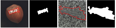
Figure 4: Examples of the inaccurate anomaly annotation in the popular MVTec AD dataset[51].

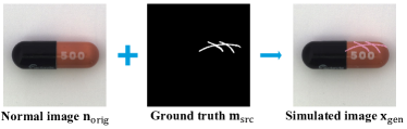
Figure 5: Illustration of anomaly generation by cut-paste.

IV-A1 Dataset

Many popular datasets suffer from inaccurate pixel-level annotations of GTs [32]. For example, Fig. 4 illustrates two examples in the MVTec AD dataset [51], where the GTs cover more normal regions. To avoid it, this paper creates a new dataset based on the MVTec AD dataset to ensure precise annotations. Following the cut-paste strategy [33, 40], which is widely adopted for anomaly generation, we first randomly pick a normal image $\mathbf{n}_{\mathrm{orig}}$ from the original MVTec AD dataset. Then, a defective image $\mathbf{x}_{\mathrm{gen}}$ is generated as:

$$\mathbf{x}_{\mathrm{gen}}=(\mathbf{1}-\mathbf{m}_{\mathrm{src}})\odot\mathbf{n}_{\mathrm{orig}}+\mathbf{m}_{\mathrm{src}}\odot\mathbf{a}_{\mathrm{src}},$$ (16)

where $\odot$ indicates the element-wise multiplication, $\mathbf{a}_{\mathrm{src}}$ and $\mathbf{m}_{\mathrm{src}}$ are anomaly source and mask source respectively. Fig. 5 illustrates the above procedure. For $\mathbf{a}_{\mathrm{src}}$, we simply select a random color . $\mathbf{m}_{\mathrm{src}}$ is first selected from the MVTec AD dataset and then randomly resized. Notably, for the pixel $(i,j)$ with $\mathbf{m}_{\mathrm{src},i,j}=1$, it is required that $\mathbf{x}_{\mathrm{gen},i,j}$ and $\mathbf{n}_{\mathrm{orig},i,j}$ are also far from each other. If not satisfied, we change $\mathbf{x}_{\mathrm{gen},i,j}$ by multiplying a desired factor.

Finally, three categories of textures (Wood, Leather, Tile) and objects (Hazelnut, Metal nut, Capsule) are created. The number of training samples ranges from 165 to 337, and 54 testing samples are generated for each category.

IV-A2 Evaluation Metrics

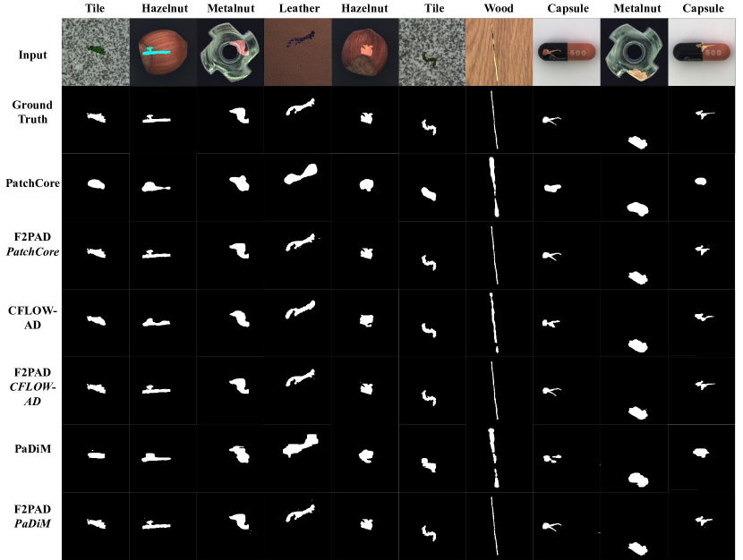
Figure 6: Visualization of comparative results. Each row from top to bottom represents the input image, GT, the detection results of PatchCore, F2PAD based on PatchCore, CFLOW-AD, F2PAD based on CFLOW-AD, PaDiM, F2PAD based on PaDiM, respectively.

To better evaluate the accuracy of the anomaly boundaries detected by these methods, we choose the Intersection over Union (IOU) and DICE coefficient to evaluate our F2PAD, which are widely adopted in image segmentation tasks:

$$\mathrm{DICE}=2\frac{|\mathbf{m}\cap\mathbf{m}_{\mathrm{gt}}|}{|\mathbf{m}|+|\mathbf{m}_{\mathrm{gt}}|},\ \mathrm{IOU}=\frac{|\mathbf{m}\cap\mathbf{m}_{\mathrm{gt}}|}{|\mathbf{m}\cup\mathbf{m}_{\mathrm{gt}}|},$$ (17)

where $\mathbf{m}_{\mathrm{gt}}$ is the GT mask. Furthermore, we multiply IOU and DICE by 100 for better illustration. Notably, higher IOU and DICE indicate better results of pixel-level anomaly segmentation.

TABLE I: Comparative results of our F2PAD and original backbone methods in the normal setting ($\Delta$: The difference in a metric between F2PAD and the original backbone).

Category	PatchCore		F2PAD PatchCore				CFLOW-AD		F2PAD CFLOW-AD				PaDiM		F2PAD PaDiM
	IOU	DICE	IOU	$\Delta$	DICE	$\Delta$	IOU	DICE	IOU	$\Delta$	DICE	$\Delta$	IOU	DICE	IOU	$\Delta$	DICE	$\Delta$
Hazelnut	67.5	80.1	86.9	19.5$\uparrow$	92.5	12.4$\uparrow$	76.0	86.1	86.3	10.3$\uparrow$	91.8	5.7$\uparrow$	65.3	78.5	88.3	23.0$\uparrow$	93.6	15.1$\uparrow$
Leather	70.4	82.1	91.9	21.4$\uparrow$	95.7	13.6$\uparrow$	77.9	87.4	91.9	14.0$\uparrow$	95.4	8.0$\uparrow$	61.6	75.6	93.2	31.6$\uparrow$	96.4	20.8$\uparrow$
Metal nut	71.5	83.0	89.4	17.9$\uparrow$	93.7	10.7$\uparrow$	78.4	87.4	89.3	10.9$\uparrow$	93.8	6.4$\uparrow$	68.9	81.3	91.1	22.2$\uparrow$	95.0	13.7$\uparrow$
Capsule	60.6	74.6	86.1	25.5$\uparrow$	92.4	17.8$\uparrow$	68.4	80.8	83.4	15.0$\uparrow$	90.3	9.5$\uparrow$	55.3	70.4	85.5	30.2$\uparrow$	92.0	21.6$\uparrow$
Tile	69.2	81.4	95.0	25.8$\uparrow$	97.4	15.9$\uparrow$	87.1	93.0	95.4	8.3$\uparrow$	97.1	4.1$\uparrow$	64.5	78.0	96.7	32.2$\uparrow$	98.3	20.3$\uparrow$
Wood	59.9	73.5	86.6	26.7$\uparrow$	91.8	18.3$\uparrow$	70.0	81.8	90.5	20.5$\uparrow$	94.3	12.4$\uparrow$	51.2	66.6	87.5	36.2$\uparrow$	92.2	25.6$\uparrow$
Mean	66.5	79.1	89.3	22.8$\uparrow$	93.9	14.8$\uparrow$	76.3	86.1	89.5	13.2$\uparrow$	93.8	7.7$\uparrow$	61.1	75.1	90.4	29.3$\uparrow$	94.6	19.5$\uparrow$

IV-A3 Implementation Details

Each image is resized to $224\times 224$ before model training and testing. Following the official implementations , Resnet18 is chosen as the feature extractor for PaDiM and PatchCore, while EfficientNet-B6 is for CFLOW-AD. For PatchCore, $|\mathcal{M}_{i,j}|=50$ for all $i,j$. For CFLOW-AD, we only consider the first two feature maps in the few-shot setting to avoid overfitting, see Section IV-B2. For all backbone methods, we choose the optimal thresholds of anomaly scores that maximize F1 scores to obtain their binary anomaly masks, following [13]. We fix $\epsilon=0.0001$ in $l_{a}({\mathbf{a}})$ and $\alpha^{2}=0.0001$ for $l_{p}^{2}({\mathbf{n}})$.

Moreover, our empirical results show that a small $\beta$ in (12) is required for large anomalies. Hence, instead of adopting a constant $\beta$ for different sizes of anomalies, we set $\beta=\beta_{0}/\sum_{i,j}\mathbf{m}^{(0)}_{i,j}$, where the denominator indicates the estimated anomaly size by backbone methods. We fine-tune the hyperparameters $\alpha^{1}$ and $\beta_{0}$, along with the number of components in MOG, by grid-search for each category.

For our proposed algorithm in Section III-D, $\gamma_{0}$, $k_{s}$, $\sigma_{0}$, and $\sigma_{1}$ are set as 1.0, 5, 1.1, and 3.0, respectively. Additionally, we apply the gradient clipping to $\textbf{g}_{i,j}$ by 0.03 to avoid too large values. We use the recommended parameters of Adan [49]. The optimization terminates when the loss decreases between two subsequent iterations less than 0.1 for PaDiM and 0.05 for other backbones, or running exceeds 1200 iterations. Additionally, we also penalize the pixel values to be valid during optimization.

Finally, for our ablation study in Section IV-C1, we obtain the binary mask of initialization by thresholding the pixel difference in the $l_{2}$ norm between the input and recovered images by inpainting at 0.2 .

IV-B Results

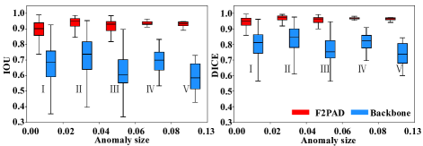
Figure 7: Results of F2PAD (red) and all backbone methods (blue) across various anomaly sizes over the whole dataset. Group I includes samples with anomaly sizes ranging from 0 to 0.02, while Group V represents those with anomaly sizes above 0.08.

IV-B1 Normal Setting

Table I presents the results of our F2PAD when applied to PatchCore, PaDiM, and CFLOW-AD, demonstrating a significant improvement of IOU and DICE in all 6 categories. The columns of $\Delta$ in Table I show the differences in IOU and DICE between F2PAD and the original backbones. Moreover, we visualize the results of 10 representative samples in Fig. 6. Though the feature-based methods can localize the anomalies as illustrated in Fig. 6, the detected anomalies exhibit inaccurate boundaries with relatively low IOU and DICE. For example, Table I shows that the original PatchCore method only achieves an average IOU of 66.5 points and DICE of 79.1 points respectively. In contrast, our F2PAD can obtain more accurate anomaly segmentation results as demonstrated by Fig. 6 and Table I, improving the IOU and DICE of PatchCore to 89.3 points and 93.9 points respectively. Similarly, our F2PAD results in improvements of 13.2 and 7.7 points in IOU and DICE for CFLOW-AD, respectively, and 29.3 and 19.5 points for PaDiM, respectively. The improvements benefit from our model (12), which directly handles Issues 1&2 of feature-based methods, as discussed in Section I.

In addition, Fig. 7 summarizes the results across all categories and backbones concerning anomaly size. It categorizes samples into five groups (I to V), based on anomaly sizes within the intervals from [0, 0.02] to [0.08, 0.13], respectively. Here, anomaly size refers to the ratio of the anomaly area to the total image area, with 0.13 being the largest anomaly size in our dataset. Fig. 7 demonstrates the consistent improvements of our F2PAD over different sizes of anomalies.

TABLE II: Comparative results of our F2PAD and original backbone methods in the few-shot setting with only 16 images for training ($\Delta$: The difference in a metric between F2PAD and the original backbone).

Category	PatchCore		F2PAD PatchCore				CFLOW-AD		F2PAD CFLOW-AD				PaDiM		F2PAD PaDiM
	IOU	DICE	IOU	$\Delta$	DICE	$\Delta$	IOU	DICE	IOU	$\Delta$	DICE	$\Delta$	IOU	DICE	IOU	$\Delta$	DICE	$\Delta$
Hazelnut	66.9	79.6	85.8	18.9$\uparrow$	92.2	12.6$\uparrow$	67.3	79.9	84.5	17.2$\uparrow$	90.7	10.8$\uparrow$	63.8	77.5	88.2	24.5$\uparrow$	92.7	15.3$\uparrow$
Leather	70.3	82.1	90.9	20.6$\uparrow$	94.7	12.7$\uparrow$	70.6	82.5	91.2	20.6$\uparrow$	94.8	12.3$\uparrow$	66.9	79.7	89.5	22.7$\uparrow$	92.9	13.2$\uparrow$
Metal nut	70.9	82.6	91.1	20.2$\uparrow$	95.3	12.7$\uparrow$	63.4	76.6	87.5	24.1$\uparrow$	92.5	15.9$\uparrow$	67.9	80.5	88.8	20.8$\uparrow$	92.6	12.1$\uparrow$
Capsule	60.1	74.2	83.6	23.5$\uparrow$	90.3	16.2$\uparrow$	44.9	60.8	69.0	24.1$\uparrow$	78.2	17.5$\uparrow$	57.1	71.9	86.1	29.0$\uparrow$	92.4	20.5$\uparrow$
Tile	68.7	81.1	94.8	26.1$\uparrow$	97.3	16.2$\uparrow$	73.6	84.5	93.4	19.7$\uparrow$	96.3	11.8$\uparrow$	66.5	79.5	89.1	22.6$\uparrow$	93.7	14.3$\uparrow$
Wood	59.7	73.2	87.8	28.1$\uparrow$	92.3	19.1$\uparrow$	63.2	77.0	89.2	25.9$\uparrow$	93.4	16.4$\uparrow$	57.4	71.6	86.0	28.6$\uparrow$	91.3	19.7$\uparrow$
Mean	66.1	78.8	89.0	22.9$\uparrow$	93.7	14.9$\uparrow$	63.8	76.9	85.8	22.0$\uparrow$	91.0	14.1$\uparrow$	63.3	76.8	88.0	24.7$\uparrow$	92.6	15.9$\uparrow$

IV-B2 Few-Shot Setting

One benefit of feature-based methods is their less demand for the sample size in training, particularly relevant in real manufacturing scenarios with small-batch production. Therefore, we provide the few-shot setting to validate the performance of our F2PAD under the above scenario. Specifically, we only use 16 samples for each category during training, as suggested in [19], while the test dataset adopted in Section IV-B1 remains unchanged. The results are summarized in Table II. Due to the more challenging setting, the performance of the backbone methods decreases slightly, as shown in Table II. Nevertheless, our F2PAD still achieves significant improvement in IOU and DICE for all backbones and categories.

In conclusion, our F2PAD can successfully handle three backbones in various data categories and apply to normal and few-shot settings.

IV-C Ablation Study

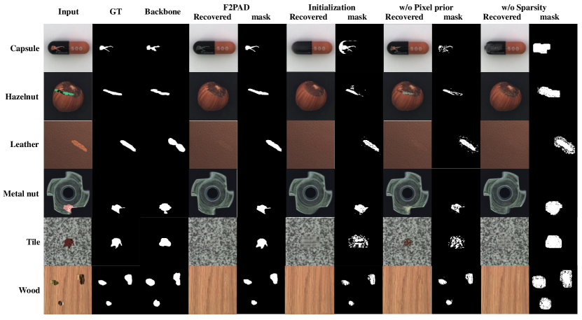
Figure 8: Visualization of the results of ablation study on initialization and regularization terms. Each column from left to right represents the input image, GT, the mask obtained by original backbone methods, the recovered non-defective images and masks obtained by F2PAD, initialization, F2PAD without the pixel prior $l_{p}(\mathbf{n})$, and F2PAD without the sparsity-inducing penalty $l_{a}(\mathbf{a})$, respectively.

TABLE III: Ablation study of initialization and regularization over the whole dataset.

Type	F2PAD PatchCore		F2PAD CFLOW-AD		F2PAD PaDiM
	IOU	DICE	IOU	DICE	IOU	DICE
Initialization	71.9	82.0	71.9	82.1	71.9	82.0
w/o Pixel prior	72.6	82.0	71.4	80.8	69.9	79.7
w/o Sparsity	32.6	48.6	32.5	48.5	28.8	44.2
F2PAD	89.3	93.9	89.5	93.8	90.4	94.6

IV-C1 Comparison with Initialization

We first demonstrate the effectiveness of our optimization model (12), compared to the initial solution obtained by inpainting as discussed in Section III-E1. The results of IOU and DICE are presented in Table III, where the final solution of (12) improves IOU and DICE by above 17.4 points (PatchCore) and 11.7 points (CFLOW-AD) respectively. Furthermore, Fig. 8 showcases visualized results for six samples across diverse categories. The recovered images of initialization lose certain textural details. For example, the random spots of Tile are heavily obscured, as shown in Fig. 8. Moreover, the initialization may also generate incompatible structures with target objects. For example, the bottom tooth of the Metal nut in Fig. 8 is significantly warped. The reason for the above phenomena is that we adopt the large pretrained model for image inpainting to obtain the initial solution, it lacks sufficient domain knowledge to ensure precise reconstruction of unseen objects in manufacturing scenarios. Therefore, the inaccuracies at the pixel level are inevitable. However, the initial solution can initialize the further optimization of our F2PAD, leading to satisfactory pixel-level anomaly segmentation, as illustrated in Figs. 6 and 8.

IV-C2 Importance of Regularization

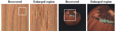
Figure 9: Illustration of the corrupted pixels in the recovered images (Wood and Hazelnut) of Fig. 8 without the pixel prior term, where we enlarge the regions within the white rectangles in the right columns.

This part discusses the importance of the pixel prior term $l_{p}(\mathbf{n})$ and the sparsity-inducing penalty $l_{a}(\mathbf{a})$ in our model (3). Concretely, we remove $l_{p}(\mathbf{n})$ and $l_{n}(\mathbf{n})$ respectively, denoted as w/o Pixel prior and w/o Sparsity in Table III and Fig. 8. Table III shows a decrease of IOU and DICE if removing the two regularization terms.

As discussed in Section III-C2, the pixel prior $l_{p}(\mathbf{n})$ plays an important role in recovering the pixel values. As illustrated in Fig. 8, the anomaly masks generated without incorporating pixel priors are incomplete, with discernible missing areas within their interior regions. To understand it, Fig. 9 enlarges the anomalous regions of recovered images, showing heavily corrupted pixels similar to the color noise. Although these corrupted pixels may not distort the semantic information too much, the integrity of anomaly masks at the pixel level will deteriorate. Moreover, the uncertainties associated with the corrupted pixels also complicate the optimization process, making it more challenging and unstable. In contrast, by incorporating the pixel prior, our F2PAD obtains more complete anomaly masks and realistic non-defective images, as shown in Fig. 8.

Finally, the sparsity-inducing penalty $l_{a}(\mathbf{a})$ enables accurate anomaly segmentation by restricting the locality of anomalies. As shown in Fig. 8, the results without sparsity cannot identify the anomaly boundaries, which cover more normal regions and thus result in the lowest IOU and DICE in Table III.

IV-C3 Performance of Optimization Algorithm

We show the superiority of our proposed optimization algorithm in Section III-D to the original Adan [49]. We provide an example from the Tile category in Fig. 10 when applied to PatchCore. The bottom-left plot in Fig. 10 (a) illustrates that some normal pixels are mislabeled in the result obtained by the original Adan. This observation indicates that these pixels are early-stopped during optimization, consistent with the higher loss value in Fig. 10 (b). In contrast, thanks to the local gradient-sharing mechanism in Section IV-C3, our proposed algorithm converges into a lower loss value and thus provides a more accurate anomaly mask, as shown in Fig. 10.

Overall, both our model as defined in (3), the regularization terms, and the proposed optimization algorithm are critical for our method to enable precise pixel-level anomaly segmentation.

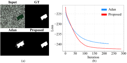
Figure 10: Visualization of the results obtained by our proposed optimization algorithm and standard Adan [49] with an example from the Tile category when applied to PatchCore. (a) From top-left to bottom-right, the input image, GT, and masks are displayed, respectively. (b) Loss trajectories during the optimization process.

V Conclusion

Unsupervised image anomaly detection is critical for various manufacturing applications, where precise pixel-level anomaly segmentation is required for downstream tasks. However, existing feature-based methods show inaccurate anomaly boundaries due to the decreased resolution of the feature map and the mixture of adjacent normal and anomalous pixels. To address the above issues, we proposed a novel optimization framework, namely F2PAD, to enhance various feature-based methods, including the popular PatchCore, CFLOW-AD, and PaDiM. Our extensive case studies demonstrated that our F2PAD improved remarkably over three backbone methods in normal and few-shot settings. Moreover, the necessity of each component in F2PAD was demonstrated by our ablation studies. Our F2PAD is suitable to handle realistic and complex manufacturing scenarios, such as small-batch manufacturing, and has the potential to become a general framework to enhance feature-based anomaly detection methods.

Chengyu Tao is pursuing his PhD degree in the Individualized Interdisciplinary Program in Smart Manufacturing with the Academy of Interdisciplinary Studies, The Hong Kong University of Science and Technology, Hong Kong SAR, China. His research interests focus on industrial data analytics, including anomaly detection and quality control of manufacturing systems.

Hao Xu is an MPhil student from the Smart Manufacturing Thrust, Systems Hub, The Hong Kong University of Science and Technology (Guangzhou), starting in 2022fall. He received his bachelor’s degree in Materials Processing from Chongqing University in 2020 and his MSc degree in Data Science from City University of Hong Kong in 2022. His research focuses on anomaly detection in the manufacturing industry utilizing weakly supervised and unsupervised learning.

Juan Du is currently an Assistant Professor with the Smart Manufacturing Thrust, Systems Hub, The Hong Kong University of Science and Technology (Guangzhou), China. She is also affiliated with the Department of Mechanical and Aerospace Engineering, The Hong Kong University of Science and Technology, Hong Kong SAR, China, and Guangzhou HKUST Fok Ying Tung Research Institute, Guangzhou, China. Her current research interests include data analytics and machine learning for modeling, monitoring, control, diagnosis and optimization in smart manufacturing systems. Dr. Du is a senior member of the Institute of Industrial and Systems Engineers (IISE), and a member of the Institute for Operations Research and the Management Sciences (INFORMS), the American Society of Mechanical Engineers (ASME), and the Society of Manufacturing Engineers (SME).

References

- [1] D. Tabernik, S. Šela, J. Skvarč, and D. Skočaj, “Segmentation based deep learning approach for surface defect detection,” Journal of Intelligent Manufacturing, vol. 31, pp. 759–776, 2019.
- [2] J. Silvestre-Blanes, T. Albero-Albero, I. Miralles, R. Pérez-Llorens, and J. Moreno, “A public fabric database for defect detection methods and results,” Autex Research Journal, vol. 19, no. 4, pp. 363–374, 2019.
- [3] X. Tao, X. Gong, X. Zhang, S. Yan, and C. Adak, “Deep learning for unsupervised anomaly localization in industrial images: A survey,” IEEE Transactions on Instrumentation and Measurement, vol. 71, pp. 1–21, 2022.
- [4] P. Bergmann, M. Fauser, D. Sattlegger, and C. Steger, “MVTec AD – A comprehensive real-world dataset for unsupervised anomaly detection,” in Proceedings of the IEEE/CVF Conference on Computer Vision and Pattern Recognition, June 2019.
- [5] S. Satorres Martínez, J. Gómez Ortega, J. Gámez García, and A. Sánchez García, “A machine vision system for defect characterization on transparent parts with non-plane surfaces,” Machine Vision and Applications, vol. 23, pp. 1–13, 2012.
- [6] A. Yadollahi, M. Mahtabi, A. Khalili, H. Doude, and J. Newman Jr, “Fatigue life prediction of additively manufactured material: Effects of surface roughness, defect size, and shape,” Fatigue & Fracture of Engineering Materials & Structures, vol. 41, no. 7, pp. 1602–1614, 2018.
- [7] Y. Wang, W. Sun, J. Jin, Z. Kong, and X. Yue, “MVGCN: multi-view graph convolutional neural network for surface defect identification using three-dimensional point cloud,” Journal of Manufacturing Science and Engineering, vol. 145, no. 3, p. 031004, 2023.
- [8] J. Liu, G. Xie, J. Wang, S. Li, C. Wang, F. Zheng, and Y. Jin, “Deep industrial image anomaly detection: A survey,” arXiv e-prints, pp. arXiv–2301, 2023.
- [9] P. Bergmann, S. Löwe, M. Fauser, D. Sattlegger, and C. Steger, “Improving unsupervised defect segmentation by applying structural similarity to autoencoders,” arXiv preprint arXiv:1807.02011, 2018.
- [10] V. Zavrtanik, M. Kristan, and D. Skočaj, “Draem-a discriminatively trained reconstruction embedding for surface anomaly detection,” in Proceedings of the IEEE/CVF International Conference on Computer Vision, 2021, pp. 8330–8339.
- [11] J. Song, K. Kong, Y.-I. Park, S.-G. Kim, and S.-J. Kang, “Anoseg: anomaly segmentation network using self-supervised learning,” arXiv preprint arXiv:2110.03396, 2021.
- [12] J. Deng, W. Dong, R. Socher, L.-J. Li, K. Li, and L. Fei-Fei, “Imagenet: A large-scale hierarchical image database,” in 2009 IEEE Conference on Computer Vision and Pattern Recognition. Ieee, 2009, pp. 248–255.
- [13] T. Defard, A. Setkov, A. Loesch, and R. Audigier, “Padim: a patch distribution modeling framework for anomaly detection and localization,” in International Conference on Pattern Recognition. Springer, 2021, pp. 475–489.
- [14] O. Rippel, P. Mertens, and D. Merhof, “Modeling the distribution of normal data in pre-trained deep features for anomaly detection,” in 2020 25th International Conference on Pattern Recognition. IEEE, 2021, pp. 6726–6733.
- [15] M. Rudolph, B. Wandt, and B. Rosenhahn, “Same same but differnet: Semi-supervised defect detection with normalizing flows,” in Proceedings of the IEEE/CVF Winter Conference on Applications of Computer Vision, 2021, pp. 1907–1916.
- [16] D. Gudovskiy, S. Ishizaka, and K. Kozuka, “CFLOW-AD: Real-time unsupervised anomaly detection with localization via conditional normalizing flows,” in Proceedings of the IEEE/CVF Winter Conference on Applications of Computer Vision, 2022, pp. 98–107.
- [17] P. Bergmann, M. Fauser, D. Sattlegger, and C. Steger, “Uninformed students: Student-teacher anomaly detection with discriminative latent embeddings,” in Proceedings of the IEEE/CVF Conference on Computer Vision and Pattern Recognition, 2020, pp. 4183–4192.
- [18] S. Mou, M. Cao, H. Bai, P. Huang, J. Shi, and J. Shan, “PAEDID: Patch autoencoder-based deep image decomposition for pixel-level defective region segmentation,” IISE Transactions, pp. 1–15, 2023.
- [19] K. Roth, L. Pemula, J. Zepeda, B. Schölkopf, T. Brox, and P. Gehler, “Towards total recall in industrial anomaly detection,” in Proceedings of the IEEE/CVF Conference on Computer Vision and Pattern Recognition, 2022, pp. 14 318–14 328.
- [20] K. He, X. Zhang, S. Ren, and J. Sun, “Deep residual learning for image recognition,” in Proceedings of the IEEE Conference on Computer Cision and Pattern Recognition, 2016, pp. 770–778.
- [21] A. Dosovitskiy, L. Beyer, A. Kolesnikov, D. Weissenborn, X. Zhai, T. Unterthiner, M. Dehghani, M. Minderer, G. Heigold, S. Gelly, et al., “An image is worth 16x16 words: Transformers for image recognition at scale,” arXiv preprint arXiv:2010.11929, 2020.
- [22] J. Yi and S. Yoon, “Patch SVDD: Patch-level SVDD for anomaly detection and segmentation,” in Proceedings of the Asian Conference on Computer Vision, 2020.
- [23] L. Wang, D. Zhang, J. Guo, and Y. Han, “Image anomaly detection using normal data only by latent space resampling,” Applied Sciences, vol. 10, no. 23, p. 8660, 2020.
- [24] A.-S. Collin and C. De Vleeschouwer, “Improved anomaly detection by training an autoencoder with skip connections on images corrupted with stain-shaped noise,” in 2020 25th International Conference on Pattern Recognition. IEEE, 2021, pp. 7915–7922.
- [25] H. Xu, J. Du, and A. Wang, “Ano-sups: Multi-size anomaly detection for manufactured products by identifying suspected patches,” arXiv preprint arXiv:2309.11120, 2023.
- [26] Y. Lee and P. Kang, “AnoViT: Unsupervised anomaly detection and localization with vision transformer-based encoder-decoder,” IEEE Access, vol. 10, pp. 46 717–46 724, 2022.
- [27] J. Pirnay and K. Chai, “Inpainting transformer for anomaly detection,” in International Conference on Image Analysis and Processing. Springer, 2022, pp. 394–406.
- [28] J. Balzategui, L. Eciolaza, and D. Maestro-Watson, “Anomaly detection and automatic labeling for solar cell quality inspection based on generative adversarial network,” Sensors, vol. 21, no. 13, p. 4361, 2021.
- [29] J. Wyatt, A. Leach, S. M. Schmon, and C. G. Willcocks, “Anoddpm: Anomaly detection with denoising diffusion probabilistic models using simplex noise,” in Proceedings of the IEEE/CVF Conference on Computer Vision and Pattern Recognition, 2022, pp. 650–656.
- [30] Y. Teng, H. Li, F. Cai, M. Shao, and S. Xia, “Unsupervised visual defect detection with score-based generative model,” arXiv preprint arXiv:2211.16092, 2022.
- [31] D. Dehaene, O. Frigo, S. Combrexelle, and P. Eline, “Iterative energy-based projection on a normal data manifold for anomaly localization,” in International Conference on Learning Representations, 2020. [Online]. Available: https://openreview.net/forum?id=HJx81ySKwr
- [32] S. Mou, X. Gu, M. Cao, H. Bai, P. Huang, J. Shan, and J. Shi, “RGI: robust GAN-inversion for mask-free image inpainting and unsupervised pixel-wise anomaly detection,” arXiv preprint arXiv:2302.12464, 2023.
- [33] A. Bauer, “Self-supervised training with autoencoders for visual anomaly detection,” arXiv preprint arXiv:2206.11723, 2022.
- [34] J. Yu, Y. Zheng, X. Wang, W. Li, Y. Wu, R. Zhao, and L. Wu, “Fastflow: Unsupervised anomaly detection and localization via 2D normalizing flows,” arXiv preprint arXiv:2111.07677, 2021.
- [35] N. Cohen and Y. Hoshen, “Sub-image anomaly detection with deep pyramid correspondences,” arXiv preprint arXiv:2005.02357, 2020.
- [36] M. Xu, X. Zhou, X. Gao, W. He, and S. Niu, “Discriminative feature learning framework with gradient preference for anomaly detection,” IEEE Transactions on Instrumentation and Measurement, vol. 72, pp. 1–10, 2022.
- [37] Z. Zhang and X. Deng, “Anomaly detection using improved deep svdd model with data structure preservation,” Pattern Recognition Letters, vol. 148, pp. 1–6, 2021.
- [38] M. Salehi, N. Sadjadi, S. Baselizadeh, M. H. Rohban, and H. R. Rabiee, “Multiresolution knowledge distillation for anomaly detection,” in Proceedings of the IEEE/CVF Conference on Computer Vision and Pattern Recognition, 2021, pp. 14 902–14 912.
- [39] C. Bailer, T. Habtegebrial, D. Stricker, et al., “Fast feature extraction with cnns with pooling layers,” arXiv preprint arXiv:1805.03096, 2018.
- [40] J. Bae, J.-H. Lee, and S. Kim, “Pni: industrial anomaly detection using position and neighborhood information,” in Proceedings of the IEEE/CVF International Conference on Computer Vision, 2023, pp. 6373–6383.
- [41] A. Paszke, S. Gross, S. Chintala, G. Chanan, E. Yang, Z. DeVito, Z. Lin, A. Desmaison, L. Antiga, and A. Lerer, “Automatic differentiation in pytorch,” 2017.
- [42] C. Tao and J. Du, “Pointsgrade: Sparse learning with graph representation for anomaly detection by using unstructured 3D point cloud data,” IISE Transactions, no. just-accepted, pp. 1–22, 2023.
- [43] H. Yan, K. Paynabar, and J. Shi, “Anomaly detection in images with smooth background via smooth-sparse decomposition,” Technometrics, vol. 59, no. 1, pp. 102–114, 2017.
- [44] D. Mo, W. K. Wong, Z. Lai, and J. Zhou, “Weighted double-low-rank decomposition with application to fabric defect detection,” IEEE Transactions on Automation Science and Engineering, vol. 18, no. 3, pp. 1170–1190, 2020.
- [45] X. Cao, C. Tao, and J. Du, “3D-CSAD: Untrained 3D anomaly detection for complex manufacturing surfaces,” arXiv preprint arXiv:2404.07748, 2024.
- [46] C. Ke, M. Ahn, S. Shin, and Y. Lou, “Iteratively reweighted group lasso based on log-composite regularization,” SIAM Journal on Scientific Computing, vol. 43, no. 5, pp. S655–S678, 2021.
- [47] H. Attias, “A variational baysian framework for graphical models,” Advances in Neural Information Processing Systems, vol. 12, 1999.
- [48] T. Miyata, “Inter-channel relation based vectorial total variation for color image recovery,” in 2015 IEEE International Conference on Image Processing. IEEE, 2015, pp. 2251–2255.
- [49] X. Xie, P. Zhou, H. Li, Z. Lin, and S. Yan, “Adan: Adaptive nesterov momentum algorithm for faster optimizing deep models,” ArXiv, vol. abs/2208.06677, 2022.
- [50] K. He, X. Chen, S. Xie, Y. Li, P. Dollár, and R. Girshick, “Masked autoencoders are scalable vision learners,” in Proceedings of the IEEE/CVF Conference on Computer Vision and Pattern Recognition, 2022, pp. 16 000–16 009.
- [51] P. Bergmann, M. Fauser, D. Sattlegger, and C. Steger, “MVTec AD–a comprehensive real-world dataset for unsupervised anomaly detection,” in Proceedings of the IEEE/CVF Conference on Computer Vision and Pattern Recognition, 2019, pp. 9592–9600.