Deformation of invariant tori under perturbation

Abstract

This study extends the functional perturbation theory, originally developed for orbits and periodic orbits in dynamical systems, e.g. a map $\mathcal{P}$, to derive formulae for the deformation of an $d$-dimensional invariant torus, on which one can define $\mathcal{P}^{k}$ for $k\in\mathbb{R}$ and even $\mathbf{\bm{k}}\in\mathbb{R}^{d}$ to continuize and generalize the exponential function $\mathcal{P}^{\mathbf{\bm{k}}}$ in $k$. The invariant tori, which manifest as closed flux surfaces in magnetic confinement fusion (MCF) machines, are the dominant structure influencing the radial transport and, consequently, the overall confinement performance.

Introduction.—

Invariant tori constitute the ordered components of a conservative dynamical system, such as a Hamiltonian system, as opposed to the chaotic components where the long-term future is unpredictable. The greater the number of integral invariants in a Hamiltonian system, the more space is occupied by invariant tori, and the more integrable the system is considered.

In MCF machines, the nested closed flux surfaces being invariant tori are essential to pursue optimal performance since these surfaces dominate the radial transport of charged particles, but can be threatened by the plasma response, the complicated current re-distribution caused by plasma-wall interaction, and disruptions due to the collapse of these surfaces [1, 2, 3, 4, 5, 6, 7].

Efforts to mitigate or suppress edge localized modes (ELMs) by resonant magnetic perturbations (RMP) [8, 9, 10, 11, 12, 13, 14] heavily relies on the flux coordinates $(r,\theta,\phi)$ constructed on the unperturbed well-nested flux surfaces without gaps, which inherently possess singularities at $r=0$ and $r=1$, and fail in the presence of chaos or emerging island chains. In contrast, the angle coordinates in this Letter are established directly as functions, $\mathbf{\bm{\theta}}=\mathbf{\bm{\theta}}[\mathcal{P}](\mathbf{\bm{x}})$, of the system and the location, dynamically changing in a way conforming to the system without errors in transforming between $\mathbf{\bm{\theta}}$ and $\mathbf{\bm{x}}$.

Preserving the confined volume surrounded by the last closed flux surface (LCFS) is necessitated by the realistic economic consideration for a fusion reactor based on the fact that the cost needed for the space inside the vacuum vessel per cubic meter is expensive. On the other hand, the stickiness of the LCFS is suspected to influence the flux of particles crossing it, which acts as the separatrix, into the scrape-off layer. [15, 16, 17]

Predicting the deformation of invariant tori is crucial for understanding system behaviour under perturbations. This understanding aids in designing optimized systems and anticipating outcomes without the need for costly or impractical real-world perturbations, e.g. the impact of long-period comets on the Solar System.

The destruction of invariant tori, a central topic in Kolmogorov-Arnold-Moser (KAM) theorem research, is closely related to their deformation. Complex patterns like an island-around-island hierarchy and cantori with infinite gaps emerge as invariant tori are destroyed [15, 18, 19, 20]. This Letter provides a foundational basis for more in-depth studies on these phenomena.

Deduction and demonstration.—

This Letter follows the conventional definition of invariant torus: for a map $\mathcal{P}:\mathbb{R}^{n}\rightarrow\mathbb{R}^{n}$, if there exists a diffeomorphism: $\mathbf{\bm{\varphi}}:\mathbb{R}^{n}\supset\mathcal{T}^{d}\rightarrow\mathbb{T}^{d}$ ($\mathbb{T}^{d}$ is the standard $d$-torus) such that the resulting motion on $\mathbb{T}^{d}$ is uniform linear but not static, i.e. $\mathbf{\bm{\varphi}}(\mathcal{P}(\mathbf{\bm{x}}))-\mathbf{\bm{\varphi}}(\mathbf{\bm{x}})=\Delta\mathbf{\bm{\theta}}\in\mathbb{R}^{d}\setminus\{\mathbf{\bm{0}}\}$ is constant, then $\mathcal{T}^{d}$ is called a $d$-dimensinoal invariant torus (or invariant $d$-torus) and $\Delta\mathbf{\bm{\theta}}$ is called a rotation vector of $\mathcal{T}^{d}$, while the corresponding frequency vector is $\mathbf{\bm{m}}:=[2\pi/\Delta\theta_{1},\dots,2\pi/\Delta\theta_{d}]$, following the convention in MCF community that field lines on a flux surface with a rotation transform $\iota=n/m=1/q$ ($n$ and $m$ are coprime) run $m$ toroidal turns to return. Note that $\Delta\mathbf{\bm{\theta}}$ is not unique for $d\geq 2$. An invariant torus with a commensurable rotation vector is called an $\mathbf{\bm{\omega}}$-commensurable invariant torus, otherwise an $\mathbf{\bm{\omega}}$-incommensurable one.

Let $\mathbf{\bm{{\mathchoice{\raisebox{0.0pt}{$\displaystyle\chi$}}{\raisebox{0.0pt}{$\textstyle\chi$}}{\raisebox{0.0pt}{$\scriptstyle\chi$}}{\raisebox{0.0pt}{$\scriptscriptstyle\chi$}}}}}(\theta_{1},\dots,\theta_{d})$ be a parameterization of $\mathcal{T}^{d}$, obeying $\mathcal{P}(\mathbf{\bm{{\mathchoice{\raisebox{0.0pt}{$\displaystyle\chi$}}{\raisebox{0.0pt}{$\textstyle\chi$}}{\raisebox{0.0pt}{$\scriptstyle\chi$}}{\raisebox{0.0pt}{$\scriptscriptstyle\chi$}}}}}(\theta_{1},\dots,\theta_{d}))=\mathbf{\bm{{\mathchoice{\raisebox{0.0pt}{$\displaystyle\chi$}}{\raisebox{0.0pt}{$\textstyle\chi$}}{\raisebox{0.0pt}{$\scriptstyle\chi$}}{\raisebox{0.0pt}{$\scriptscriptstyle\chi$}}}}}(\theta_{1}+\Delta\theta_{1},\dots,\theta_{d}+\Delta\theta_{d})$, based on which one can let a vector $\mathbf{\bm{k}}$ be the exponent of the map $\mathcal{P}$ to continuize and generalize $\mathcal{P}^{k}$ from $k\in\mathbb{Z}$ to $\mathbf{\bm{k}}\in\mathbb{R}^{d}$,

$$\mathcal{P}^{\mathbf{\bm{k}}}\left(\mathbf{\bm{{\mathchoice{\raisebox{0.0pt}{$\displaystyle\chi$}}{\raisebox{0.0pt}{$\textstyle\chi$}}{\raisebox{0.0pt}{$\scriptstyle\chi$}}{\raisebox{0.0pt}{$\scriptscriptstyle\chi$}}}}}(\mathbf{\bm{\theta}})\right):=\mathbf{\bm{{\mathchoice{\raisebox{0.0pt}{$\displaystyle\chi$}}{\raisebox{0.0pt}{$\textstyle\chi$}}{\raisebox{0.0pt}{$\scriptstyle\chi$}}{\raisebox{0.0pt}{$\scriptscriptstyle\chi$}}}}}(\mathbf{\bm{\theta}}+\mathbf{\bm{k}}\!\ast\!\Delta\mathbf{\bm{\theta}}),$$ (1)

where $\!\ast\!$ denotes the element-wise multiplication. Then $\mathcal{P}^{\mathbf{\bm{m}}}$ is by definition a returning map on $\mathcal{T}^{d}$. In the case $k\in\mathbb{R}$ instead of $\mathbb{R}^{d}$, $\mathbf{\bm{k}}\!\ast\!\Delta\mathbf{\bm{\theta}}$ degrades to $k\Delta\mathbf{\bm{\theta}}$.

When $d=n-1$, a series of nested invariant $(n-1)$-tori can then be parameterized as $\mathbf{\bm{{\mathchoice{\raisebox{0.0pt}{$\displaystyle\chi$}}{\raisebox{0.0pt}{$\textstyle\chi$}}{\raisebox{0.0pt}{$\scriptstyle\chi$}}{\raisebox{0.0pt}{$\scriptscriptstyle\chi$}}}}}(\mathbf{\bm{\theta}},r)$ where $r$ is the torus label and is commonly understood as the radial direction. The case of $d=n-1$ is assumed from now on. For readers focusing on Hamiltonian systems, an $n$ degree-of-freedom Hamiltonian system has a $2n$-D phase space and may have at most $n$ integral invariants $\{I_{i}\}$, leading to that those researchers may adopt $n$ torus labels, e.g. $I_{i}$, if they need an invertible $\mathbf{\bm{{\mathchoice{\raisebox{0.0pt}{$\displaystyle\chi$}}{\raisebox{0.0pt}{$\textstyle\chi$}}{\raisebox{0.0pt}{$\scriptstyle\chi$}}{\raisebox{0.0pt}{$\scriptscriptstyle\chi$}}}}}(\mathbf{\bm{\theta}},\mathbf{\bm{r}})$.

Be aware that $\mathbf{\bm{{\mathchoice{\raisebox{0.0pt}{$\displaystyle\chi$}}{\raisebox{0.0pt}{$\textstyle\chi$}}{\raisebox{0.0pt}{$\scriptstyle\chi$}}{\raisebox{0.0pt}{$\scriptscriptstyle\chi$}}}}}(\mathbf{\bm{\theta}},r)$ may be merely defined on a fragmented set $\mathcal{F}\subset\mathbb{R}$ due to the deviation of the system from integrability, for which the derivative in $r$ is allowed to be defined in a weaker form than the regular one,

$$\frac{\partial}{\partial r}\mathbf{\bm{{\mathchoice{\raisebox{0.0pt}{$\displaystyle\chi$}}{\raisebox{0.0pt}{$\textstyle\chi$}}{\raisebox{0.0pt}{$\scriptstyle\chi$}}{\raisebox{0.0pt}{$\scriptscriptstyle\chi$}}}}}(\mathbf{\bm{\theta}},r):=\lim_{\begin{subarray}{c}r^{\prime}\rightarrow r\\ r^{\prime}\in\mathcal{F}\end{subarray}}\frac{\mathbf{\bm{{\mathchoice{\raisebox{0.0pt}{$\displaystyle\chi$}}{\raisebox{0.0pt}{$\textstyle\chi$}}{\raisebox{0.0pt}{$\scriptstyle\chi$}}{\raisebox{0.0pt}{$\scriptscriptstyle\chi$}}}}}(\mathbf{\bm{\theta}},r^{\prime})-\mathbf{\bm{{\mathchoice{\raisebox{0.0pt}{$\displaystyle\chi$}}{\raisebox{0.0pt}{$\textstyle\chi$}}{\raisebox{0.0pt}{$\scriptstyle\chi$}}{\raisebox{0.0pt}{$\scriptscriptstyle\chi$}}}}}(\mathbf{\bm{\theta}},r_{i})}{r^{\prime}-r}.$$ (2)

The definition of $\nabla$ is also relaxed because variables e.g. $\mathbf{\bm{\theta}}(\mathbf{\bm{x}})$ and $r(\mathbf{\bm{x}})$ may only be defined on a fragmented subset of $\mathbb{R}^{n}$.

$\partial_{k}\mathcal{P}^{k}$ can then be easily computed by the $\mathbf{\bm{\theta}}$ grid. $\partial_{k}\mathcal{P}^{k}=\partial\mathbf{\bm{{\mathchoice{\raisebox{0.0pt}{$\displaystyle\chi$}}{\raisebox{0.0pt}{$\textstyle\chi$}}{\raisebox{0.0pt}{$\scriptstyle\chi$}}{\raisebox{0.0pt}{$\scriptscriptstyle\chi$}}}}}/\partial\mathbf{\bm{\theta}}|_{\mathbf{\bm{\theta}}+k\Delta\mathbf{\bm{\theta}}}\cdot\Delta\mathbf{\bm{\theta}}=\sum_{i=1}^{d}\Delta\theta_{i}~{}\partial\mathbf{\bm{{\mathchoice{\raisebox{0.0pt}{$\displaystyle\chi$}}{\raisebox{0.0pt}{$\textstyle\chi$}}{\raisebox{0.0pt}{$\scriptstyle\chi$}}{\raisebox{0.0pt}{$\scriptscriptstyle\chi$}}}}}/\partial\theta_{i}|_{\mathbf{\bm{\theta}}+k\Delta\mathbf{\bm{\theta}}}$, and

$$\partial_{\mathbf{\bm{k}}}\mathcal{P}^{\mathbf{\bm{k}}} =\frac{\partial\mathbf{\bm{{\mathchoice{\raisebox{0.0pt}{$\displaystyle\chi$}}{\raisebox{0.0pt}{$\textstyle\chi$}}{\raisebox{0.0pt}{$\scriptstyle\chi$}}{\raisebox{0.0pt}{$\scriptscriptstyle\chi$}}}}}}{\partial\mathbf{\bm{\theta}}}\Bigg{|}_{\mathrlap{\smash{\mathbf{\bm{\theta}}+\mathbf{\bm{k}}\!\ast\!\Delta\mathbf{\bm{\theta}}}}}\cdot\overbrace{\frac{\partial(\mathbf{\bm{k}}\!\ast\!\Delta\mathbf{\bm{\theta}})}{\partial\mathbf{\bm{k}}}}^{\mathrlap{=\operatorname{diag}(\Delta\mathbf{\bm{\theta}})_{d\times d}}}=\left.\begin{bmatrix}\mid&&\mid\\ \Delta\theta_{1}\partial_{\theta_{1}}\mathbf{\bm{{\mathchoice{\raisebox{0.0pt}{$\displaystyle\chi$}}{\raisebox{0.0pt}{$\textstyle\chi$}}{\raisebox{0.0pt}{$\scriptstyle\chi$}}{\raisebox{0.0pt}{$\scriptscriptstyle\chi$}}}}}&\cdots&\Delta\theta_{d}\partial_{\theta_{d}}\mathbf{\bm{{\mathchoice{\raisebox{0.0pt}{$\displaystyle\chi$}}{\raisebox{0.0pt}{$\textstyle\chi$}}{\raisebox{0.0pt}{$\scriptstyle\chi$}}{\raisebox{0.0pt}{$\scriptscriptstyle\chi$}}}}}\\ \mid&&\mid\end{bmatrix}\right|_{\mathrlap{\smash{\mathbf{\bm{\theta}}+\mathbf{\bm{k}}\!\ast\!\Delta\mathbf{\bm{\theta}}}}}$$ (3)

As powerful mathematical tools introduced from functional analysis, partial and total functional derivatives are denoted by $\delta/\delta\mathcal{B}$ and $\mathrm{d}/\mathrm{d}\mathcal{B}$, which become directional derivatives $\Delta\mathcal{B}\cdot\delta/\delta\mathcal{B}$ and $\Delta\mathcal{B}\cdot\mathrm{d}/\mathrm{d}\mathcal{B}$ when accompanied by a given perturbation. For brevity, the former one can be simply denoted $\delta$ if the system to be perturbed and the perturbation are clear.

The shift of a periodic orbit on invariant $d$-tori under perturbation $\Delta\mathcal{P}$, as the aim of this Letter, can not be solved by the simple geometry analysis for hyperbolic periodic orbits given in [21]

$$\delta\mathbf{\bm{x}}_{\text{cyc}} =-\left[\mathcal{D}\mathcal{P}^{\mathbf{\bm{m}}}-\mathbf{I}\right]^{-1}\cdot\delta\mathcal{P}^{\mathbf{\bm{m}}},$$ (4)

where $\mathcal{D}\mathcal{P}^{\mathbf{\bm{m}}}-\mathbf{I}$ has eigenvalue(s) equal to zero(s) leading to its non-inversibility. The root cause is that the parallel component of $\delta\mathbf{\bm{x}}_{\text{cyc}}$ can take an arbitrary value, for which one has to return to the geometric analysis

$$\delta\mathbf{\bm{x}}_{\text{cyc}} =\delta\mathcal{P}^{\mathbf{\bm{m}}}(\mathbf{\bm{x}}_{\text{cyc}})+\mathcal{D}\mathcal{P}^{\mathbf{\bm{m}}}(\mathbf{\bm{x}}_{\text{cyc}})\cdot\delta\mathbf{\bm{x}}_{\text{cyc}},$$ (5)

to replace $$\delta\mathbf{\bm{x}}_{\text{cyc}} \delta_{\perp}:=\sum_{i=1}^{n-d}\hat{\mathbf{\bm{n}}}_{i}\hat{\mathbf{\bm{n}}}_{i}^{\text{T}}\cdot\delta \{\hat{\mathbf{\bm{n}}}_{i}\}_{i=1}^{n-d} \bm{N}_{p}\mathcal{T}^{d}$$ with , where is an orthonormal basis of the local normal space .

$$\text{Then, }\delta_{\perp}\mathbf{\bm{x}}_{\text{cyc}} =\delta\mathcal{P}^{\mathbf{\bm{m}}}(\mathbf{\bm{x}}_{\text{cyc}})+\mathcal{D}\mathcal{P}^{\mathbf{\bm{m}}}(\mathbf{\bm{x}}_{\text{cyc}})\cdot\delta_{\perp}\mathbf{\bm{x}}_{\text{cyc}},$$ (6)

However, another problem arises: $(\mathcal{D}\mathcal{P}^{\mathbf{\bm{m}}}-\mathbf{I})\cdot\delta_{\perp}\mathbf{\bm{x}}_{\text{cyc}}$ can only have a parallel component if $\mathcal{D}\mathcal{P}^{\mathbf{\bm{m}}}$ has all eigenvalues equal to one, which is usually the case for flux-preserving maps. Then, either $\delta\mathcal{P}^{\mathbf{\bm{m}}}(\mathbf{\bm{x}}_{\text{cyc}})$ has only a parallel component to $\mathcal{T}^{d}$, or the $\mathcal{D}\mathcal{P}^{\mathbf{\bm{m}}}$ eigenvalue(s) corresponding to the eigenvectors not tangent to $\mathcal{T}^{d}$ are allowed to deviate from one, or the invariant torus is to be destroyed, leading to that $\delta_{\perp}\mathbf{\bm{x}}_{\text{cyc}}$ becomes meaningless. A short answer for the first case can be immediately acquired by imposing the functional total derivative $\Delta\mathcal{P}\cdot\mathrm{d}/\mathrm{d}\mathcal{P}$ on both sides of the equation defining the returning map $\mathcal{P}^{\mathbf{\bm{m}}}$,

$$\mathcal{P}^{\mathbf{\bm{m}}[\mathcal{P}](\mathbf{\bm{x}})}[\mathcal{P}](\mathbf{\bm{x}}):=\mathbf{\bm{x}},$$ (7)

$$\underbrace{\partial_{\mathbf{\bm{m}}}\mathcal{P}^{\mathbf{\bm{m}}}\cdot\delta\mathbf{\bm{m}}}_{\mathrlap{{=\sum_{i=1}^{d}\partial_{\theta_{i}}\!\mathbf{\bm{{\mathchoice{\raisebox{0.0pt}{$\displaystyle\chi$}}{\raisebox{0.0pt}{$\textstyle\chi$}}{\raisebox{0.0pt}{$\scriptstyle\chi$}}{\raisebox{0.0pt}{$\scriptscriptstyle\chi$}}}}}~{}\Delta\theta_{i}\delta m_{i}}}}+\delta\mathcal{P}^{\mathbf{\bm{m}}}=\mathbf{\bm{0}},$$ (8)

which clearly shows that $\delta\mathcal{P}^{\mathbf{\bm{m}}}$ must be tangent to $\mathcal{T}^{d}$ if the returning map $\mathcal{P}^{\mathbf{\bm{m}}}$ remains well-defined under perturbation.

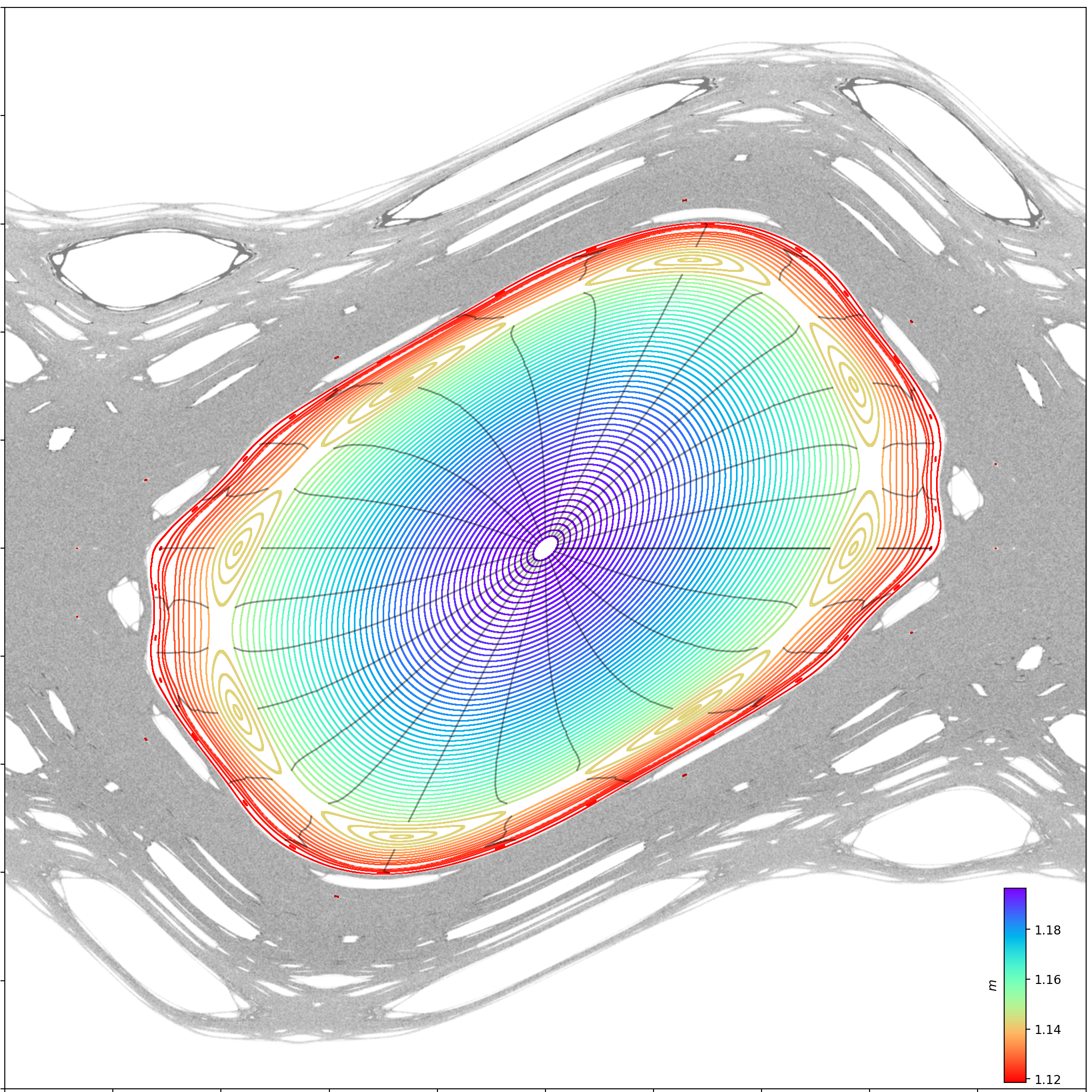
Figure 1: Distribution of $m$ for the Chirikov standard map at $k=0.975$ for $\mathbf{\bm{x}}\in[-0.5,0.5]\times[-0.5,0.5]$.

Take the standard map as a demonstration of the formulae in this Letter, setting $p=0.975$ (the same as Fig. 1 in [20]). To determine the exponent $m$ such that $\mathcal{P}^{m}$ is a returning map for points on an irrational invariant torus, map the initial point $\mathbf{\bm{x}}_{0}$ for numerous times. Define an angle difference $\Delta\theta\in[0,2\pi)$ for once mapping, then $\mathbf{\bm{x}}_{i}$ compared to $\mathbf{\bm{x}}_{0}$ has an angle difference $i\Delta\theta$. Denote how many times the orbit crosses $\mathbf{\bm{x}}_{0}$ counterclockwise until the $i$-th point by $n_{i}$, then one knows the angle increment $i\Delta\theta$ from $\mathbf{\bm{x}}_{0}$ to $\mathbf{\bm{x}}_{i}$ is between $2\pi n_{i}\leq i\Delta\theta\leq 2\pi(n_{i}+1)$. Notice $m=2\pi/\Delta\theta$, therefore

$$\frac{i}{n_{i}+1}\leq m\leq\frac{i}{n_{i}},\quad\forall i\in\mathbb{N}$$ (9)

The two variable needed to solve for $\delta_{\perp}\mathbf{\bm{x}}_{\text{cyc}}$ by Eq. (6) are $\mathcal{D}\mathcal{P}^{\mathbf{\bm{m}}}$ and $\delta\mathcal{P}^{\mathbf{\bm{m}}}$. An expression of $\mathcal{D}\mathcal{P}^{\mathbf{\bm{k}}}$ in terms of $\partial_{r}\mathbf{\bm{{\mathchoice{\raisebox{0.0pt}{$\displaystyle\chi$}}{\raisebox{0.0pt}{$\textstyle\chi$}}{\raisebox{0.0pt}{$\scriptstyle\chi$}}{\raisebox{0.0pt}{$\scriptscriptstyle\chi$}}}}}$ and $\partial_{\mathbf{\bm{\theta}}}\mathbf{\bm{{\mathchoice{\raisebox{0.0pt}{$\displaystyle\chi$}}{\raisebox{0.0pt}{$\textstyle\chi$}}{\raisebox{0.0pt}{$\scriptstyle\chi$}}{\raisebox{0.0pt}{$\scriptscriptstyle\chi$}}}}}$ is acquired by exerting total derivatives in $r$ and $\mathbf{\bm{\theta}}$ resp. on the equation (1) defining $\mathcal{P}^{\mathbf{\bm{k}}}$,

$$\mathcal{D}\mathcal{P}^{\mathbf{\bm{k}}}\left(\mathbf{\bm{{\mathchoice{\raisebox{0.0pt}{$\displaystyle\chi$}}{\raisebox{0.0pt}{$\textstyle\chi$}}{\raisebox{0.0pt}{$\scriptstyle\chi$}}{\raisebox{0.0pt}{$\scriptscriptstyle\chi$}}}}}(\mathbf{\bm{\theta}},r)\right)\cdot\partial_{r}\mathbf{\bm{{\mathchoice{\raisebox{0.0pt}{$\displaystyle\chi$}}{\raisebox{0.0pt}{$\textstyle\chi$}}{\raisebox{0.0pt}{$\scriptstyle\chi$}}{\raisebox{0.0pt}{$\scriptscriptstyle\chi$}}}}}(\mathbf{\bm{\theta}},r)=\partial_{r}\mathbf{\bm{{\mathchoice{\raisebox{0.0pt}{$\displaystyle\chi$}}{\raisebox{0.0pt}{$\textstyle\chi$}}{\raisebox{0.0pt}{$\scriptstyle\chi$}}{\raisebox{0.0pt}{$\scriptscriptstyle\chi$}}}}}(\mathbf{\bm{\theta}}+\mathbf{\bm{k}}\!\ast\!\Delta\mathbf{\bm{\theta}},r)$$ (10)

$$+\partial_{\mathbf{\bm{\theta}}}\mathbf{\bm{{\mathchoice{\raisebox{0.0pt}{$\displaystyle\chi$}}{\raisebox{0.0pt}{$\textstyle\chi$}}{\raisebox{0.0pt}{$\scriptstyle\chi$}}{\raisebox{0.0pt}{$\scriptscriptstyle\chi$}}}}}(\mathbf{\bm{\theta}}+\mathbf{\bm{k}}\!\ast\!\Delta\mathbf{\bm{\theta}},r)\cdot\left(\mathbf{\bm{k}}\!\ast\!\frac{\mathrm{d}\Delta\mathbf{\bm{\theta}}}{\mathrm{d}r}\right),$$

$$\mathcal{D}\mathcal{P}^{\mathbf{\bm{k}}}\left(\mathbf{\bm{{\mathchoice{\raisebox{0.0pt}{$\displaystyle\chi$}}{\raisebox{0.0pt}{$\textstyle\chi$}}{\raisebox{0.0pt}{$\scriptstyle\chi$}}{\raisebox{0.0pt}{$\scriptscriptstyle\chi$}}}}}(\mathbf{\bm{\theta}},r)\right)\cdot\partial_{\mathbf{\bm{\theta}}}\mathbf{\bm{{\mathchoice{\raisebox{0.0pt}{$\displaystyle\chi$}}{\raisebox{0.0pt}{$\textstyle\chi$}}{\raisebox{0.0pt}{$\scriptstyle\chi$}}{\raisebox{0.0pt}{$\scriptscriptstyle\chi$}}}}}(\mathbf{\bm{\theta}},r)=\partial_{\mathbf{\bm{\theta}}}\mathbf{\bm{{\mathchoice{\raisebox{0.0pt}{$\displaystyle\chi$}}{\raisebox{0.0pt}{$\textstyle\chi$}}{\raisebox{0.0pt}{$\scriptstyle\chi$}}{\raisebox{0.0pt}{$\scriptscriptstyle\chi$}}}}}(\mathbf{\bm{\theta}}+\mathbf{\bm{k}}\!\ast\!\Delta\mathbf{\bm{\theta}},r),$$ (11)

$$\mathcal{D}\mathcal{P}^{\mathbf{\bm{k}}}\left(\mathbf{\bm{{\mathchoice{\raisebox{0.0pt}{$\displaystyle\chi$}}{\raisebox{0.0pt}{$\textstyle\chi$}}{\raisebox{0.0pt}{$\scriptstyle\chi$}}{\raisebox{0.0pt}{$\scriptscriptstyle\chi$}}}}}(\mathbf{\bm{\theta}},r)\right)=\left.\begin{bmatrix}\begin{array}[]{l}\partial_{\mathbf{\bm{\theta}}}\mathbf{\bm{{\mathchoice{\raisebox{0.0pt}{$\displaystyle\chi$}}{\raisebox{0.0pt}{$\textstyle\chi$}}{\raisebox{0.0pt}{$\scriptstyle\chi$}}{\raisebox{0.0pt}{$\scriptscriptstyle\chi$}}}}}\cdot(\mathbf{\bm{k}}\!\ast\!\frac{\mathrm{d}\Delta\mathbf{\bm{\theta}}}{\mathrm{d}r})\\ +\partial_{r}\mathbf{\bm{{\mathchoice{\raisebox{0.0pt}{$\displaystyle\chi$}}{\raisebox{0.0pt}{$\textstyle\chi$}}{\raisebox{0.0pt}{$\scriptstyle\chi$}}{\raisebox{0.0pt}{$\scriptscriptstyle\chi$}}}}}\end{array}&\partial_{\mathbf{\bm{\theta}}}\mathbf{\bm{{\mathchoice{\raisebox{0.0pt}{$\displaystyle\chi$}}{\raisebox{0.0pt}{$\textstyle\chi$}}{\raisebox{0.0pt}{$\scriptstyle\chi$}}{\raisebox{0.0pt}{$\scriptscriptstyle\chi$}}}}}\end{bmatrix}\right|_{\mathrlap{\mathbf{\bm{\theta}}+\mathbf{\bm{k}}\!\ast\!\Delta\mathbf{\bm{\theta}}}}\cdot\left.\begin{bmatrix}\partial_{r}\mathbf{\bm{{\mathchoice{\raisebox{0.0pt}{$\displaystyle\chi$}}{\raisebox{0.0pt}{$\textstyle\chi$}}{\raisebox{0.0pt}{$\scriptstyle\chi$}}{\raisebox{0.0pt}{$\scriptscriptstyle\chi$}}}}}&\partial_{\mathbf{\bm{\theta}}}\mathbf{\bm{{\mathchoice{\raisebox{0.0pt}{$\displaystyle\chi$}}{\raisebox{0.0pt}{$\textstyle\chi$}}{\raisebox{0.0pt}{$\scriptstyle\chi$}}{\raisebox{0.0pt}{$\scriptscriptstyle\chi$}}}}}\end{bmatrix}\right|_{\mathrlap{\mathbf{\bm{\theta}}}}^{-1}$$

$$=\left.\begin{bmatrix}\mid&\mid~{}\mid\mid\mid~{}\mid\\ \begin{array}[]{l}\partial_{\mathbf{\bm{\theta}}}\mathbf{\bm{{\mathchoice{\raisebox{0.0pt}{$\displaystyle\chi$}}{\raisebox{0.0pt}{$\textstyle\chi$}}{\raisebox{0.0pt}{$\scriptstyle\chi$}}{\raisebox{0.0pt}{$\scriptscriptstyle\chi$}}}}}\cdot(\mathbf{\bm{k}}\!\ast\!\frac{\mathrm{d}\Delta\mathbf{\bm{\theta}}}{\mathrm{d}r})\end{array}&\mathbf{0}_{n\times(n-1)}\\ \mid&\mid~{}\mid\mid\mid~{}\mid\end{bmatrix}\right|_{\mathrlap{\mathbf{\bm{\theta}}+\mathbf{\bm{k}}\!\ast\!\Delta\mathbf{\bm{\theta}}}}\cdot\left.\begin{bmatrix}\partial_{r}\mathbf{\bm{{\mathchoice{\raisebox{0.0pt}{$\displaystyle\chi$}}{\raisebox{0.0pt}{$\textstyle\chi$}}{\raisebox{0.0pt}{$\scriptstyle\chi$}}{\raisebox{0.0pt}{$\scriptscriptstyle\chi$}}}}}&\partial_{\mathbf{\bm{\theta}}}\mathbf{\bm{{\mathchoice{\raisebox{0.0pt}{$\displaystyle\chi$}}{\raisebox{0.0pt}{$\textstyle\chi$}}{\raisebox{0.0pt}{$\scriptstyle\chi$}}{\raisebox{0.0pt}{$\scriptscriptstyle\chi$}}}}}\end{bmatrix}\right|_{\mathrlap{\mathbf{\bm{\theta}}}}^{-1}+\mathbf{I}_{n\times n}.$$

Note the inverse of $[\partial_{r}\mathbf{\bm{{\mathchoice{\raisebox{0.0pt}{$\displaystyle\chi$}}{\raisebox{0.0pt}{$\textstyle\chi$}}{\raisebox{0.0pt}{$\scriptstyle\chi$}}{\raisebox{0.0pt}{$\scriptscriptstyle\chi$}}}}}~{}~{}\partial_{\mathbf{\bm{\theta}}}\mathbf{\bm{{\mathchoice{\raisebox{0.0pt}{$\displaystyle\chi$}}{\raisebox{0.0pt}{$\textstyle\chi$}}{\raisebox{0.0pt}{$\scriptstyle\chi$}}{\raisebox{0.0pt}{$\scriptscriptstyle\chi$}}}}}]$ is $\begin{bmatrix}-~{}\nabla r~{}-\\ \equiv\nabla\mathbf{\bm{\theta}}\equiv\end{bmatrix}$ so that

$$\mathcal{D}\mathcal{P}^{\mathbf{\bm{k}}}(\mathbf{\bm{{\mathchoice{\raisebox{0.0pt}{$\displaystyle\chi$}}{\raisebox{0.0pt}{$\textstyle\chi$}}{\raisebox{0.0pt}{$\scriptstyle\chi$}}{\raisebox{0.0pt}{$\scriptscriptstyle\chi$}}}}}(\mathbf{\bm{\theta}},r)) =\left.\left(\partial_{\mathbf{\bm{\theta}}}\mathbf{\bm{{\mathchoice{\raisebox{0.0pt}{$\displaystyle\chi$}}{\raisebox{0.0pt}{$\textstyle\chi$}}{\raisebox{0.0pt}{$\scriptstyle\chi$}}{\raisebox{0.0pt}{$\scriptscriptstyle\chi$}}}}}\cdot(\mathbf{\bm{k}}\!\ast\!\frac{\mathrm{d}\Delta\mathbf{\bm{\theta}}}{\mathrm{d}r})\right)\right|_{\mathrlap{\smash{\begin{subarray}{l}\mathbf{\bm{\theta}}+\mathbf{\bm{k}}\!\ast\!\Delta\mathbf{\bm{\theta}}\\ n\times 1\end{subarray}}}}~{}~{}~{}~{}~{}\nabla r\Big{|}_{\begin{subarray}{l}\mathbf{\bm{\theta}}\\ 1\times n\end{subarray}}+\mathbf{I}_{n\times n},$$ (12)

of which a special case is when $$\mathbf{\bm{k}} \mathbf{\bm{m}}$$ takes the value of ,

$$\mathcal{D}\mathcal{P}^{\mathbf{\bm{m}}}(\mathbf{\bm{x}}) =\left(\partial_{\mathbf{\bm{\theta}}}\mathbf{\bm{{\mathchoice{\raisebox{0.0pt}{$\displaystyle\chi$}}{\raisebox{0.0pt}{$\textstyle\chi$}}{\raisebox{0.0pt}{$\scriptstyle\chi$}}{\raisebox{0.0pt}{$\scriptscriptstyle\chi$}}}}}\cdot(\mathbf{\bm{m}}\!\ast\!\frac{\mathrm{d}\Delta\mathbf{\bm{\theta}}}{\mathrm{d}r})\right)\nabla r+\mathbf{I},$$ (13)

where all the variables are evaluated at $\mathbf{\bm{x}}$, therefore it is needless to indicate where to evaluate.

The eigenvalues of $\mathcal{D}\mathcal{P}^{\mathbf{\bm{m}}}$ are identical at all points of an ($\mathbf{\bm{\omega}}$-incommensurable) invariant torus. Some properties, e.g. the last statement, can be transferred between an $\mathbf{\bm{\omega}}$-commensurable torus and an $\mathbf{\bm{\omega}}$-incommensurable torus, because in most cases the former one can be considered as a limit of a sequence of the latter ones nearby and vice versa. However, there exist extreme counterexamples in which the transfer is hindered, e.g. an isolated invariant torus which has no invariant torus nearby.

Be careful that $\mathcal{D}\mathcal{P}^{\mathbf{\bm{k}}}(\mathbf{\bm{x}})$ is not $\mathbf{\bm{m}}$-periodic in $k$ as $\mathcal{P}^{k}$ is, which is because points on nearby invariant tori are probably to be mapped away from each other due to the shear between tori, i.e. neighbouring tori have a bit different rotation vectors $\Delta\mathbf{\bm{\theta}}$. $\delta\mathcal{P}^{k}(\mathbf{\bm{x}})$ is also not $m$-periodic but due to that the impact of perturbation is accumulated all the way.

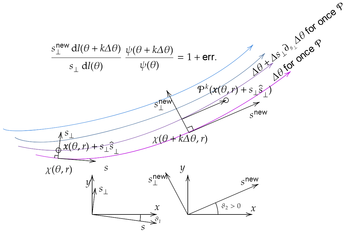
Figure 2: Cartoon to show the $\mathcal{D}\mathcal{P}^{k}$ and the local frames of coordinate systems.

The distance between two neighbouring invariant tori varies with which point to evaluate the distance. This is reflected by $\mathcal{D}\mathcal{P}^{\mathbf{\bm{m}}}$. Let $(n,d)=(2,1)$ for illustration (see Fig. 2) and this case is of great importance owing to that the distance variation also reflects the density of flux surfaces in an MCF machine. Denote a matrix representing $\varphi$ rad counterclockwise rotation in $\mathbb{R}^{2}$ by $\mathbf{R}_{\varphi}$. Construct local coordinate frames at $\mathbf{\bm{x}}$ and $\mathcal{P}^{k}(\mathbf{\bm{x}})$ resp. with orthonormal bases $\{\hat{\mathbf{\bm{s}}},\hat{\mathbf{\bm{s}}}_{\perp}\}$ and $\{\hat{\mathbf{\bm{s}}}^{\text{new}},\hat{\mathbf{\bm{s}}}_{\perp}^{\text{new}}\}$, then

$$\mathrm{d}\mathbf{\bm{x}}_{\text{loc}} =\mathbf{R}_{-\vartheta_{1}}\mathrm{d}\mathbf{\bm{x}}$$

$$\overbrace{\mathrm{d}\mathbf{\bm{x}}_{\text{loc}}^{\text{new}}}^{\mathllap{\smash{\begin{bmatrix}\mathrm{d}s^{\text{new}}\\ \mathrm{d}s_{\perp}^{\text{new}}\end{bmatrix}=~{}~{}}}} =\mathcal{D}\mathcal{P}^{k}_{\text{loc}}~{}\overbrace{\mathrm{d}\mathbf{\bm{x}}_{\text{loc}}}^{\mathrlap{\smash{\equiv\mathrm{d}s~{}\hat{\mathbf{\bm{s}}}+\mathrm{d}s_{\perp}~{}\hat{\mathbf{\bm{s}}}_{\perp}=\begin{bmatrix}\mathrm{d}s~{}~{}\\ \mathrm{d}s_{\perp}\end{bmatrix}}}}$$

$$\mathrm{d}\mathbf{\bm{x}}^{\text{new}}_{\text{loc}} =\mathbf{R}_{-\vartheta_{2}}\mathrm{d}\mathbf{\bm{x}}^{\text{new}}$$

$$\mathrm{d}\mathbf{\bm{x}}^{\text{new}} =\underbrace{\mathbf{R}_{\vartheta_{2}}\mathcal{D}\mathcal{P}^{k}_{\text{loc}}\mathbf{R}_{-\vartheta_{1}}}_{\mathrlap{\smash{=\mathcal{D}\mathcal{P}^{k}}}}\mathrm{d}\mathbf{\bm{x}}$$

where the subscripts ${}_{\text{loc}}$ mean the variables are viewed in the local frames. $\mathcal{D}\mathcal{P}^{k}_{\text{loc}}$ is deduced from Eq. (17) to be

$$\begin{bmatrix}\frac{|\partial_{\theta}\mathbf{\bm{{\mathchoice{\raisebox{0.0pt}{$\displaystyle\chi$}}{\raisebox{0.0pt}{$\textstyle\chi$}}{\raisebox{0.0pt}{$\scriptstyle\chi$}}{\raisebox{0.0pt}{$\scriptscriptstyle\chi$}}}}}|_{\theta+k\Delta\theta}}{|\partial_{\theta}\mathbf{\bm{{\mathchoice{\raisebox{0.0pt}{$\displaystyle\chi$}}{\raisebox{0.0pt}{$\textstyle\chi$}}{\raisebox{0.0pt}{$\scriptstyle\chi$}}{\raisebox{0.0pt}{$\scriptscriptstyle\chi$}}}}}|_{\theta}}&\begin{array}[]{l}(\partial_{r}\mathbf{\bm{{\mathchoice{\raisebox{0.0pt}{$\displaystyle\chi$}}{\raisebox{0.0pt}{$\textstyle\chi$}}{\raisebox{0.0pt}{$\scriptstyle\chi$}}{\raisebox{0.0pt}{$\scriptscriptstyle\chi$}}}}}\cdot\hat{\mathbf{\bm{s}}})|_{\theta+k\Delta\theta}/|\partial_{r}\mathbf{\bm{{\mathchoice{\raisebox{0.0pt}{$\displaystyle\chi$}}{\raisebox{0.0pt}{$\textstyle\chi$}}{\raisebox{0.0pt}{$\scriptstyle\chi$}}{\raisebox{0.0pt}{$\scriptscriptstyle\chi$}}}}}\cdot\hat{\mathbf{\bm{s}}}_{\perp}|_{\theta}\\ +\left.\left(k\frac{\mathrm{d}\Delta\theta}{\mathrm{d}r}-\frac{\partial_{r}\mathbf{\bm{{\mathchoice{\raisebox{0.0pt}{$\displaystyle\chi$}}{\raisebox{0.0pt}{$\textstyle\chi$}}{\raisebox{0.0pt}{$\scriptstyle\chi$}}{\raisebox{0.0pt}{$\scriptscriptstyle\chi$}}}}}\cdot\partial_{\theta}\mathbf{\bm{{\mathchoice{\raisebox{0.0pt}{$\displaystyle\chi$}}{\raisebox{0.0pt}{$\textstyle\chi$}}{\raisebox{0.0pt}{$\scriptstyle\chi$}}{\raisebox{0.0pt}{$\scriptscriptstyle\chi$}}}}}}{|\partial_{\theta}\mathbf{\bm{{\mathchoice{\raisebox{0.0pt}{$\displaystyle\chi$}}{\raisebox{0.0pt}{$\textstyle\chi$}}{\raisebox{0.0pt}{$\scriptstyle\chi$}}{\raisebox{0.0pt}{$\scriptscriptstyle\chi$}}}}}|^{2}}\right)\right|_{\theta}\cdot\frac{|\partial_{\theta}\mathbf{\bm{{\mathchoice{\raisebox{0.0pt}{$\displaystyle\chi$}}{\raisebox{0.0pt}{$\textstyle\chi$}}{\raisebox{0.0pt}{$\scriptstyle\chi$}}{\raisebox{0.0pt}{$\scriptscriptstyle\chi$}}}}}|_{\theta+k\Delta\theta}}{|\partial_{r}\mathbf{\bm{{\mathchoice{\raisebox{0.0pt}{$\displaystyle\chi$}}{\raisebox{0.0pt}{$\textstyle\chi$}}{\raisebox{0.0pt}{$\scriptstyle\chi$}}{\raisebox{0.0pt}{$\scriptscriptstyle\chi$}}}}}\cdot\hat{\mathbf{\bm{s}}}_{\perp}|_{\theta}}\end{array}\\ 0&\frac{(\partial_{r}\mathbf{\bm{{\mathchoice{\raisebox{0.0pt}{$\displaystyle\chi$}}{\raisebox{0.0pt}{$\textstyle\chi$}}{\raisebox{0.0pt}{$\scriptstyle\chi$}}{\raisebox{0.0pt}{$\scriptscriptstyle\chi$}}}}}\cdot\hat{\mathbf{\bm{s}}}_{\perp})|_{\theta+k\Delta\theta}}{|\partial_{r}\mathbf{\bm{{\mathchoice{\raisebox{0.0pt}{$\displaystyle\chi$}}{\raisebox{0.0pt}{$\textstyle\chi$}}{\raisebox{0.0pt}{$\scriptstyle\chi$}}{\raisebox{0.0pt}{$\scriptscriptstyle\chi$}}}}}\cdot\hat{\mathbf{\bm{s}}}_{\perp}|_{\theta}}\end{bmatrix}.$$

A flux-preserving property $\psi(\mathbf{\bm{x}})\mathrm{d}V(\mathbf{\bm{x}})=\psi(\mathcal{P}(\mathbf{\bm{x}}))\mathrm{d}V(\mathcal{P}(\mathbf{\bm{x}}))$ gives a first-order estimation for the distance $s_{\perp}(\theta)$ by

$$s_{\perp}(\theta) =0+\underbrace{s_{\perp}(\theta_{0})}_{\mathclap{:=s_{\perp 0}}}\underbrace{\frac{\mathrm{d}l(\theta_{0})}{\mathrm{d}l(\theta)}\frac{\psi(\theta_{0})}{\psi(\theta)}}_{\mathrlap{=\frac{\mathrm{d}s_{\perp}}{\mathrm{d}s_{\perp 0}}=\frac{|\partial_{\theta}\mathbf{\bm{{\mathchoice{\raisebox{0.0pt}{$\displaystyle\chi$}}{\raisebox{0.0pt}{$\textstyle\chi$}}{\raisebox{0.0pt}{$\scriptstyle\chi$}}{\raisebox{0.0pt}{$\scriptscriptstyle\chi$}}}}}(\theta_{0})|}{|\partial_{\theta}\mathbf{\bm{{\mathchoice{\raisebox{0.0pt}{$\displaystyle\chi$}}{\raisebox{0.0pt}{$\textstyle\chi$}}{\raisebox{0.0pt}{$\scriptstyle\chi$}}{\raisebox{0.0pt}{$\scriptscriptstyle\chi$}}}}}(\theta)|}\frac{\psi(\theta_{0})}{\psi(\theta)}}}+\mathcal{O}(|s_{\perp 0}|^{2}),$$ (14)

where $r$ can be omitted for brevity. For a general pair $(n,d)=(n,n-1)$, the flux-preserving property turns out to be a general form,

$$\left.\det\begin{bmatrix}\mid&\cdots&\mid&\mid\\ \partial_{\theta_{1}}\mathbf{\bm{{\mathchoice{\raisebox{0.0pt}{$\displaystyle\chi$}}{\raisebox{0.0pt}{$\textstyle\chi$}}{\raisebox{0.0pt}{$\scriptstyle\chi$}}{\raisebox{0.0pt}{$\scriptscriptstyle\chi$}}}}}&\cdots&\partial_{\theta_{d}}\mathbf{\bm{{\mathchoice{\raisebox{0.0pt}{$\displaystyle\chi$}}{\raisebox{0.0pt}{$\textstyle\chi$}}{\raisebox{0.0pt}{$\scriptstyle\chi$}}{\raisebox{0.0pt}{$\scriptscriptstyle\chi$}}}}}&s_{\perp}\hat{\mathbf{\bm{s}}}_{\perp}\\ \mid&\cdots&\mid&\mid\end{bmatrix}\right|_{\mathbf{\bm{\theta}}}\psi(\mathbf{\bm{\theta}})=\text{const.}$$ (15)

Hereafter, we turn from $\mathcal{D}\mathcal{P}^{\mathbf{\bm{k}}}$ to $\delta\mathcal{P}^{\mathbf{\bm{k}}}$. By regarding the location $\mathbf{\bm{x}}$ more fundamental than $(\mathbf{\bm{\theta}},r)$ and considering the whole map $\mathcal{P}$ also as an argument of $\mathbf{\bm{\theta}}$, $\Delta\mathbf{\bm{\theta}}$, $r$ and $\textstyle\chi$, the equation (1) defining $\mathcal{P}^{\mathbf{\bm{k}}}$ becomes

$$\mathcal{P}^{\mathbf{\bm{k}}}[\mathcal{P}]\Big{(}\mathbf{\bm{{\mathchoice{\raisebox{0.0pt}{$\displaystyle\chi$}}{\raisebox{0.0pt}{$\textstyle\chi$}}{\raisebox{0.0pt}{$\scriptstyle\chi$}}{\raisebox{0.0pt}{$\scriptscriptstyle\chi$}}}}}[\mathcal{P}](\mathbf{\bm{\theta}}[\mathcal{P}](\mathbf{\bm{x}}),r[\mathcal{P}](\mathbf{\bm{x}}))\Big{)}:=$$

$$\mathbf{\bm{{\mathchoice{\raisebox{0.0pt}{$\displaystyle\chi$}}{\raisebox{0.0pt}{$\textstyle\chi$}}{\raisebox{0.0pt}{$\scriptstyle\chi$}}{\raisebox{0.0pt}{$\scriptscriptstyle\chi$}}}}}[\mathcal{P}]\Big{(}\mathbf{\bm{\theta}}[\mathcal{P}](\mathbf{\bm{x}})+\mathbf{\bm{k}}\!\ast\!\Delta\mathbf{\bm{\theta}}[\mathcal{P}](\mathbf{\bm{x}}),r[\mathcal{P}](\mathbf{\bm{x}})\Big{)},$$ (16)

which after imposed $\Delta\mathcal{P}\cdot\mathrm{d}/\mathrm{d}\mathcal{P}$ becomes

$$\delta\mathcal{P}^{\mathbf{\bm{k}}}(\mathbf{\bm{x}})+\mathcal{D}\mathcal{P}^{\mathbf{\bm{k}}}(\mathbf{\bm{x}})\cdot\cancel{\left(\delta\mathbf{\bm{{\mathchoice{\raisebox{0.0pt}{$\displaystyle\chi$}}{\raisebox{0.0pt}{$\textstyle\chi$}}{\raisebox{0.0pt}{$\scriptstyle\chi$}}{\raisebox{0.0pt}{$\scriptscriptstyle\chi$}}}}}+\partial_{\mathbf{\bm{\theta}}}\mathbf{\bm{{\mathchoice{\raisebox{0.0pt}{$\displaystyle\chi$}}{\raisebox{0.0pt}{$\textstyle\chi$}}{\raisebox{0.0pt}{$\scriptstyle\chi$}}{\raisebox{0.0pt}{$\scriptscriptstyle\chi$}}}}}\cdot\delta\mathbf{\bm{\theta}}+\partial_{r}\mathbf{\bm{{\mathchoice{\raisebox{0.0pt}{$\displaystyle\chi$}}{\raisebox{0.0pt}{$\textstyle\chi$}}{\raisebox{0.0pt}{$\scriptstyle\chi$}}{\raisebox{0.0pt}{$\scriptscriptstyle\chi$}}}}}\cdot\delta r\right)}$$

$$=\delta\mathbf{\bm{{\mathchoice{\raisebox{0.0pt}{$\displaystyle\chi$}}{\raisebox{0.0pt}{$\textstyle\chi$}}{\raisebox{0.0pt}{$\scriptstyle\chi$}}{\raisebox{0.0pt}{$\scriptscriptstyle\chi$}}}}}(\mathbf{\bm{\theta}}+\mathbf{\bm{k}}\!\ast\!\Delta\mathbf{\bm{\theta}},r)+\partial_{\mathbf{\bm{\theta}}}\mathbf{\bm{{\mathchoice{\raisebox{0.0pt}{$\displaystyle\chi$}}{\raisebox{0.0pt}{$\textstyle\chi$}}{\raisebox{0.0pt}{$\scriptstyle\chi$}}{\raisebox{0.0pt}{$\scriptscriptstyle\chi$}}}}}(\mathbf{\bm{\theta}}+\mathbf{\bm{k}}\!\ast\!\Delta\mathbf{\bm{\theta}},r)\cdot\left(\delta\mathbf{\bm{\theta}}(\mathbf{\bm{x}})+\mathbf{\bm{k}}\!\ast\!\delta\Delta\mathbf{\bm{\theta}}(\mathbf{\bm{x}})\right)$$

$$+\partial_{r}\mathbf{\bm{{\mathchoice{\raisebox{0.0pt}{$\displaystyle\chi$}}{\raisebox{0.0pt}{$\textstyle\chi$}}{\raisebox{0.0pt}{$\scriptstyle\chi$}}{\raisebox{0.0pt}{$\scriptscriptstyle\chi$}}}}}(\mathbf{\bm{\theta}}+\mathbf{\bm{k}}\!\ast\!\Delta\mathbf{\bm{\theta}},r)\cdot\delta r(\mathbf{\bm{x}}),$$ (17)

where the cancelling notation is a natural result of the equation defining $\textstyle\chi$,

$$\mathbf{\bm{{\mathchoice{\raisebox{0.0pt}{$\displaystyle\chi$}}{\raisebox{0.0pt}{$\textstyle\chi$}}{\raisebox{0.0pt}{$\scriptstyle\chi$}}{\raisebox{0.0pt}{$\scriptscriptstyle\chi$}}}}}[\mathcal{P}]\Big{(}\mathbf{\bm{\theta}}[\mathcal{P}](\mathbf{\bm{x}}),r[\mathcal{P}](\mathbf{\bm{x}})\Big{)} :=\mathbf{\bm{x}}$$ (18)

being exerted $$\Delta\mathcal{P}\cdot\mathrm{d}/\mathrm{d}\mathcal{P}$$,

$$\delta\mathbf{\bm{{\mathchoice{\raisebox{0.0pt}{$\displaystyle\chi$}}{\raisebox{0.0pt}{$\textstyle\chi$}}{\raisebox{0.0pt}{$\scriptstyle\chi$}}{\raisebox{0.0pt}{$\scriptscriptstyle\chi$}}}}}+\partial_{\theta}\mathbf{\bm{{\mathchoice{\raisebox{0.0pt}{$\displaystyle\chi$}}{\raisebox{0.0pt}{$\textstyle\chi$}}{\raisebox{0.0pt}{$\scriptstyle\chi$}}{\raisebox{0.0pt}{$\scriptscriptstyle\chi$}}}}}\cdot\delta\theta+\partial_{r}\mathbf{\bm{{\mathchoice{\raisebox{0.0pt}{$\displaystyle\chi$}}{\raisebox{0.0pt}{$\textstyle\chi$}}{\raisebox{0.0pt}{$\scriptstyle\chi$}}{\raisebox{0.0pt}{$\scriptscriptstyle\chi$}}}}}\cdot\delta r =\mathbf{\bm{0}}.$$ (19)

When $\mathbf{\bm{k}}$ takes the value of $\mathbf{\bm{m}}$,

$$\delta\mathcal{P}^{\mathbf{\bm{m}}}(\mathbf{\bm{x}}) =\delta\mathbf{\bm{{\mathchoice{\raisebox{0.0pt}{$\displaystyle\chi$}}{\raisebox{0.0pt}{$\textstyle\chi$}}{\raisebox{0.0pt}{$\scriptstyle\chi$}}{\raisebox{0.0pt}{$\scriptscriptstyle\chi$}}}}}(\mathbf{\bm{\theta}},r)+\partial_{\mathbf{\bm{\theta}}}\mathbf{\bm{{\mathchoice{\raisebox{0.0pt}{$\displaystyle\chi$}}{\raisebox{0.0pt}{$\textstyle\chi$}}{\raisebox{0.0pt}{$\scriptstyle\chi$}}{\raisebox{0.0pt}{$\scriptscriptstyle\chi$}}}}}(\mathbf{\bm{\theta}},r)\cdot\left(\delta\mathbf{\bm{\theta}}(\mathbf{\bm{x}})+\mathbf{\bm{m}}\!\ast\!\delta\Delta\mathbf{\bm{\theta}}(\mathbf{\bm{x}})\right)$$

$$+\partial_{r}\mathbf{\bm{{\mathchoice{\raisebox{0.0pt}{$\displaystyle\chi$}}{\raisebox{0.0pt}{$\textstyle\chi$}}{\raisebox{0.0pt}{$\scriptstyle\chi$}}{\raisebox{0.0pt}{$\scriptscriptstyle\chi$}}}}}(\mathbf{\bm{\theta}},r)\cdot\delta r(\mathbf{\bm{x}}),$$ (20)

There are two common criteria to identify an invariant torus during perturbation. The first one is to anchor it by a fixed point $\mathbf{\bm{x}}$, which implies that $\delta r(\mathbf{\bm{x}})$ at this point always vanishes. In the meanwhile, if $\theta(\mathbf{\bm{x}})$ at this point is endowed with a constant value no matter what perturbation is imposed, $\delta\theta(\mathbf{\bm{x}})$ also vanishes. Then $\mathbf{\bm{{\mathchoice{\raisebox{0.0pt}{$\displaystyle\chi$}}{\raisebox{0.0pt}{$\textstyle\chi$}}{\raisebox{0.0pt}{$\scriptstyle\chi$}}{\raisebox{0.0pt}{$\scriptscriptstyle\chi$}}}}}(\theta(\mathbf{\bm{x}}),r(\mathbf{\bm{x}}))$ at this point is also fixed, i.e. $\delta\mathbf{\bm{{\mathchoice{\raisebox{0.0pt}{$\displaystyle\chi$}}{\raisebox{0.0pt}{$\textstyle\chi$}}{\raisebox{0.0pt}{$\scriptstyle\chi$}}{\raisebox{0.0pt}{$\scriptscriptstyle\chi$}}}}}(\theta,\phi)=0$. The equation (17) is simplified to

$$\delta\mathcal{P}^{\mathbf{\bm{k}}}(\mathbf{\bm{x}})=\delta\mathbf{\bm{{\mathchoice{\raisebox{0.0pt}{$\displaystyle\chi$}}{\raisebox{0.0pt}{$\textstyle\chi$}}{\raisebox{0.0pt}{$\scriptstyle\chi$}}{\raisebox{0.0pt}{$\scriptscriptstyle\chi$}}}}}|_{\mathbf{\bm{\theta}}+\mathbf{\bm{k}}\!\ast\!\Delta\mathbf{\bm{\theta}}}+\partial_{\mathbf{\bm{\theta}}}\mathbf{\bm{{\mathchoice{\raisebox{0.0pt}{$\displaystyle\chi$}}{\raisebox{0.0pt}{$\textstyle\chi$}}{\raisebox{0.0pt}{$\scriptstyle\chi$}}{\raisebox{0.0pt}{$\scriptscriptstyle\chi$}}}}}\Big{|}_{\mathrlap{\mathbf{\bm{\theta}}+\mathbf{\bm{k}}\!\ast\!\Delta\mathbf{\bm{\theta}}}}\cdot\left(\mathbf{\bm{k}}\!\ast\!\delta\Delta\mathbf{\bm{\theta}}(\mathbf{\bm{x}})\right),$$ (21)

where $\delta\mathcal{P}^{\mathbf{\bm{k}}}(\mathbf{\bm{x}})$ can be computed for $\mathbf{\bm{k}}=k\!\ast\!\mathbf{\bm{1}}$, $k\in\mathbb{Z}$, by the discrete-time version of the variation progression Eq. (6) in [21], while the other unknowns are $\delta\mathbf{\bm{{\mathchoice{\raisebox{0.0pt}{$\displaystyle\chi$}}{\raisebox{0.0pt}{$\textstyle\chi$}}{\raisebox{0.0pt}{$\scriptstyle\chi$}}{\raisebox{0.0pt}{$\scriptscriptstyle\chi$}}}}}$ ($2\pi$-periodic in every $\theta_{i}$) and $\delta\Delta\mathbf{\bm{\theta}}(\mathbf{\bm{x}})\in\mathbb{R}^{d}$. One can employ inference schemes to estimate the Fourier series coefficients of $\delta\mathbf{\bm{{\mathchoice{\raisebox{0.0pt}{$\displaystyle\chi$}}{\raisebox{0.0pt}{$\textstyle\chi$}}{\raisebox{0.0pt}{$\scriptstyle\chi$}}{\raisebox{0.0pt}{$\scriptscriptstyle\chi$}}}}}$ and the value of $\delta\Delta\mathbf{\bm{\theta}}(\mathbf{\bm{x}})$.

Figure 3: Shifts of $\mathbf{\bm{{\mathchoice{\raisebox{0.0pt}{$\displaystyle\chi$}}{\raisebox{0.0pt}{$\textstyle\chi$}}{\raisebox{0.0pt}{$\scriptstyle\chi$}}{\raisebox{0.0pt}{$\scriptscriptstyle\chi$}}}}}(\theta,r)$ for an invariant torus $\mathcal{T}^{1}$ labelled by a starting point $\mathbf{\bm{x}}_{0}=[.12,.0]$ at which the angle is fixed to be zero. $k_{0}=0.975$ while $\Delta k$ takes values of $.00,.02,.04,.06,.08,0.10$. (a) for the $x$ component and (b) for the $y$ component.

The second common choice of torus label, when $(n,d)=(2,1)$ or $(3,2)$, is resp. $\Delta\theta$ or $\Delta\theta_{1}/\Delta\theta_{2}$. In the former case, let $r:=\Delta\theta(\mathbf{\bm{x}})$ and endow a fixed point $\mathbf{\bm{x}}$ with a fixed angle $\theta(\mathbf{\bm{x}})$, then, Eq. (17) is simplified into

$$\delta\mathcal{P}^{k}(\mathbf{\bm{x}})=\delta\mathbf{\bm{{\mathchoice{\raisebox{0.0pt}{$\displaystyle\chi$}}{\raisebox{0.0pt}{$\textstyle\chi$}}{\raisebox{0.0pt}{$\scriptstyle\chi$}}{\raisebox{0.0pt}{$\scriptscriptstyle\chi$}}}}}|_{\theta+k\Delta\theta}+\left.\Big{(}k\partial_{\theta}\mathbf{\bm{{\mathchoice{\raisebox{0.0pt}{$\displaystyle\chi$}}{\raisebox{0.0pt}{$\textstyle\chi$}}{\raisebox{0.0pt}{$\scriptstyle\chi$}}{\raisebox{0.0pt}{$\scriptscriptstyle\chi$}}}}}+\partial_{r}\mathbf{\bm{{\mathchoice{\raisebox{0.0pt}{$\displaystyle\chi$}}{\raisebox{0.0pt}{$\textstyle\chi$}}{\raisebox{0.0pt}{$\scriptstyle\chi$}}{\raisebox{0.0pt}{$\scriptscriptstyle\chi$}}}}}\Big{)}\right|_{\mathrlap{\smash{(\theta+k\Delta\theta,r)}}}~{}\cdot\delta r(\mathbf{\bm{x}})$$ (22)

Owing to the fact that the perpendicular shift is an intrinsic property of $\mathcal{T}^{d}$, $\delta_{\perp}\mathbf{\bm{x}}_{\text{cyc}}$ shall equal $\delta_{\perp}\mathbf{\bm{{\mathchoice{\raisebox{0.0pt}{$\displaystyle\chi$}}{\raisebox{0.0pt}{$\textstyle\chi$}}{\raisebox{0.0pt}{$\scriptstyle\chi$}}{\raisebox{0.0pt}{$\scriptscriptstyle\chi$}}}}}$ when the radial label $r$ is chosen to be $\Delta\theta$.

One can also solve for $\delta\mathcal{P}^{\mathbf{\bm{m}}}$ by transfering its known value at a point. By comparing the sums to compute $\delta\mathcal{P}^{m}$ for two successive points $\mathbf{\bm{x}}_{0}$ and $\mathbf{\bm{x}}_{1}$ in an $m$-periodic orbit,

$$\delta\mathcal{P}^{m}|_{\mathbf{\bm{x}}_{0}}= \Delta\mathcal{P}|_{\mathbf{\bm{x}}_{m-1}}+\mathcal{D}\mathcal{P}|_{\mathbf{\bm{x}}_{m-1}}\cdot\Delta\mathcal{P}|_{\mathbf{\bm{x}}_{m-2}}+\cdots$$

$$\qquad+\mathcal{D}\mathcal{P}^{m-1}|_{\mathbf{\bm{x}}_{1}}\cdot\Delta\mathcal{P}|_{\mathbf{\bm{x}}_{0}},$$

$$\delta\mathcal{P}^{m}|_{\mathbf{\bm{x}}_{1}}= \Delta\mathcal{P}|_{\mathbf{\bm{x}}_{m}}+\mathcal{D}\mathcal{P}|_{\mathbf{\bm{x}}_{m}}\cdot\Delta\mathcal{P}|_{\mathbf{\bm{x}}_{m-1}}+\cdots$$

$$\qquad+\mathcal{D}\mathcal{P}^{m-1}|_{\mathbf{\bm{x}}_{2}}\cdot\Delta\mathcal{P}|_{\mathbf{\bm{x}}_{1}}$$

$$= \Delta\mathcal{P}|_{\mathbf{\bm{x}}_{m}}+\mathcal{D}\mathcal{P}|_{\mathbf{\bm{x}}_{m}}\cdot\delta\mathcal{P}^{m}|_{\mathbf{\bm{x}}_{0}}-\mathcal{D}\mathcal{P}^{m}\cdot\Delta\mathcal{P}|_{\mathbf{\bm{x}}_{0}}$$

$$= \mathcal{D}\mathcal{P}|_{\mathbf{\bm{x}}_{0}}\cdot\delta\mathcal{P}^{m}|_{\mathbf{\bm{x}}_{0}}+(\mathbf{I}-\mathcal{D}\mathcal{P}^{m})|_{\mathbf{\bm{x}}_{1}}\cdot\Delta\mathcal{P}|_{\mathbf{\bm{x}}_{0}},$$

one can conclude that for successive points $$\mathbf{\bm{x}}_{i} \mathbf{\bm{x}}_{i+1} m$$ and in an -periodic orbit,

$$\delta\mathcal{P}^{m}|_{\mathbf{\bm{x}}_{i+1}}= \mathcal{D}\mathcal{P}|_{\mathbf{\bm{x}}_{i}}\cdot\delta\mathcal{P}^{m}|_{\mathbf{\bm{x}}_{i}}+(\mathbf{I}-\mathcal{D}\mathcal{P}^{m})|_{\mathbf{\bm{x}}_{i+1}}\cdot\Delta\mathcal{P}|_{\mathbf{\bm{x}}_{i}},$$

which can be generalized to the case of $$\mathbf{\bm{x}}\in\mathcal{T}^{d}$$ as below,

$$\delta\mathcal{P}^{\mathbf{\bm{m}}}|_{\mathcal{P}(\mathbf{\bm{x}})}= \mathcal{D}\mathcal{P}|_{\mathbf{\bm{x}}}\cdot\delta\mathcal{P}^{\mathbf{\bm{m}}}|_{\mathbf{\bm{x}}}+(\mathbf{I}-\mathcal{D}\mathcal{P}^{\mathbf{\bm{m}}})|_{\mathcal{P}(\mathbf{\bm{x}})}\cdot\Delta\mathcal{P}|_{\mathbf{\bm{x}}}.$$ (23)

.

Conclusion and discussion.—

The functional perturbation theory for dynamical systems presented in [21, 22] is further developed for invariant tori and their deformation. Not necessarily every point on an invariant torus has an accurate solution for $\delta_{\perp}\mathbf{\bm{x}}_{\text{cyc}}$ due to the fact that invariant tori may only be defined on a fragmented domain both in the space of $\mathcal{P}$ and that of $\mathbf{\bm{x}}$. An invariant torus can be destroyed into an island chain or a cantorus that has infinite gaps.

To transfer these formulae from maps to flows, one usually only needs to replace the symbols as shown below,

$$\mathcal{P}(\mathbf{\bm{x}}_{0}) \mapsto\mathbf{\bm{X}}(\mathbf{\bm{x}}_{0},t)\text{ abbr. as }\mathbf{\bm{X}}_{t}(\mathbf{\bm{x}}_{0}),$$

$$\mathbf{\bm{\varphi}}(\mathcal{P}(\mathbf{\bm{x}}))-\mathbf{\bm{\varphi}}(\mathbf{\bm{x}})=\Delta\mathbf{\bm{\theta}} \mapsto\frac{\mathrm{d}\mathbf{\bm{\varphi}}(\mathbf{\bm{X}}(\mathbf{\bm{x}}_{0},t))}{\mathrm{d}t}=\mathbf{\bm{\omega}},$$

$$\mathbf{\bm{m}}:=\left[\frac{2\pi}{\Delta\theta_{1}},\dots,\frac{2\pi}{\Delta\theta_{d}}\right] \mapsto\mathbf{\bm{T}}:=\left[\frac{2\pi}{\omega_{1}},\dots,\frac{2\pi}{\omega_{d}}\right],$$

$$\mathcal{P}^{\mathbf{\bm{k}}}(\mathbf{\bm{{\mathchoice{\raisebox{0.0pt}{$\displaystyle\chi$}}{\raisebox{0.0pt}{$\textstyle\chi$}}{\raisebox{0.0pt}{$\scriptstyle\chi$}}{\raisebox{0.0pt}{$\scriptscriptstyle\chi$}}}}}(\mathbf{\bm{\theta}})):=\mathbf{\bm{{\mathchoice{\raisebox{0.0pt}{$\displaystyle\chi$}}{\raisebox{0.0pt}{$\textstyle\chi$}}{\raisebox{0.0pt}{$\scriptstyle\chi$}}{\raisebox{0.0pt}{$\scriptscriptstyle\chi$}}}}}(\mathbf{\bm{\theta}}+\mathbf{\bm{k}}\!\ast\!\Delta\mathbf{\bm{\theta}}) \mapsto\mathbf{\bm{X}}(\mathbf{\bm{{\mathchoice{\raisebox{0.0pt}{$\displaystyle\chi$}}{\raisebox{0.0pt}{$\textstyle\chi$}}{\raisebox{0.0pt}{$\scriptstyle\chi$}}{\raisebox{0.0pt}{$\scriptscriptstyle\chi$}}}}}(\mathbf{\bm{\theta}}),\mathbf{\bm{t}}):=\mathbf{\bm{{\mathchoice{\raisebox{0.0pt}{$\displaystyle\chi$}}{\raisebox{0.0pt}{$\textstyle\chi$}}{\raisebox{0.0pt}{$\scriptstyle\chi$}}{\raisebox{0.0pt}{$\scriptscriptstyle\chi$}}}}}(\mathbf{\bm{\theta}}+\mathbf{\bm{\omega}}\!\ast\!\mathbf{\bm{t}}),$$

$$\mathcal{P}^{\mathbf{\bm{m}}} \mapsto\mathbf{\bm{X}}_{\mathbf{\bm{T}}}.$$