Projection, Degeneracy, and Singularity Degree for Spectrahedra

Abstract

Facial reduction, FR, is a regularization technique for convex programs where the strict feasibility constraint qualification, CQ, fails. Though this CQ holds generically, failure is pervasive in applications such as semidefinite relaxations of hard discrete optimization problems. In this paper we relate FR to the analysis of the convergence behaviour of a semi-smooth Newton root finding method for the projection onto a spectrahedron, i.e., onto the intersection of a linear manifold and the semidefinite cone. In the process, we derive and use an elegant formula for the projection onto a face of the semidefinite cone. We show further that the ill-conditioning of the Jacobian of the Newton method near optimality characterizes the degeneracy of the nearest point in the spectrahedron. We apply the results, both theoretically and empirically, to the problem of finding nearest points to the sets of: (i) correlation matrices or the elliptope; and (ii) semidefinite relaxations of permutation matrices or the vontope, i.e., the feasible sets for the semidefinite relaxations of the max-cut and quadratic assignment problems, respectively.

Key Words: facial reduction, spectrahedra, degeneracy, Jacobian, singularity degree, elliptope, vontope.

AMS Subject Classification: 90C22, 90C25, 90C27, 90C59.

1 Introduction

Facial reduction, FR, involves a finite number of steps that regularizes convex programs where the strict feasibility constraint qualification, CQ, fails. This CQ holds generically for linear conic programs, see e.g., [17]. However, failure is pervasive in applications such as semidefinite programming, SDP, relaxations of hard discrete optimization problems, e.g., [16]. The minimum number of FR steps is the singularity degree of ${\mathcal{F}}$, $\operatorname{sd}({\mathcal{F}})$, of the program with feasible set ${\mathcal{F}}$, and it has been shown to be related to stability, error analysis, and convergence rates, see e.g., [43, 42, 13, 15]. Further generalized notions of singularity degree such as the maximum number of FR steps are studied in [29, 26] and shown to also relate to stability and convergence rates. In this paper we study $\operatorname{sd}({\mathcal{F}})$ and relations to the projection problem, or best approximation problem (BAP), onto a spectrahedron, the intersection of a linear manifold and the positive semidefinite cone in symmetric matrix space. Our main purpose is to examine the effect of failure of strict feasibility on the projection problem. In the absence of strict feasibility, we find surprising relationships between the eigenpairs of small eigenvalues of the Jacobian in our Newton method for the projection problem and finding exposing vectors for FR. We apply the results, both theoretically and empirically, to the problem of finding nearest points to the sets of: (i) correlation matrices or the elliptope; and (ii) semidefinite relaxations of permutation matrices or the vontope, i.e., the feasible sets for the semidefinite relaxations of the max-cut and quadratic assignment problems, respectively. In the process, we derive and use an elegant formula for the projection onto a face of the semidefinite cone.

1.1 Projection Problem

We work with the Euclidean space of $n\times n$ real symmetric matrices, $\mathbb{S}^{n}$, equipped with the trace inner product. Let the data, $W\in\mathbb{S}^{n}$, be given. The projection, or basic best approximation problem, BAP, is

$$\begin{array}[]{rcll}\textit{$X^{*}$}=&\operatorname{\arg\min}&\frac{1}{2}\|X-W\|^{2},&\quad\qquad\textit{$p^{*}=\frac{1}{2}\|X^{*}-W\|^{2}$},\\ &\text{s.t.}&X\in{\mathcal{L}}\cap\mathbb{S}_{+}^{n},\end{array}$$ (1.1)

where $\mathbb{S}_{+}^{n}\subseteq\mathbb{S}^{n}$ is the closed convex cone of semidefinite matrices in the vector space of real symmetric matrices of order $n$ equipped with the trace inner product. We let $X\succeq 0$ denote $X\in\mathbb{S}_{+}^{n}$. Here ${\mathcal{L}}\subseteq\mathbb{S}^{n}$ is a linear manifold; and, $p^{*},X^{*}$ are the optimal value and optimum, respectively. The representation of the linear manifold is essential in algorithms and different representations can result in different stability properties for the problem, e.g., [46]. We let ${\mathcal{L}}=\{X\in\mathbb{S}^{n}:{\mathcal{A}}X=b\}$, where ${\mathcal{A}}:\mathbb{S}^{n}\to\mathbb{R}^{m}$ is a given surjective (without loss of generality) linear transformation; ${\mathcal{A}}X=(\tr A_{i}X)\in\mathbb{R}^{m}$ for given fixed linearly independent $A_{i}\in\mathbb{S}^{n},i=1\ldots,m$. We let ${\mathcal{F}}:={\mathcal{L}}\cap\mathbb{S}_{+}^{n}\neq\emptyset$ denote the nonempty feasible set; it is called a spectrahedron. Here the data of BAP is $W,{\mathcal{A}},b$. (In the linear programming, LP, case, $\mathbb{S}^{n}\leftarrow\mathbb{R}^{n},\mathbb{S}_{+}^{n}\leftarrow\mathbb{R}_{+}^{n}$.)

Nearest point problems are pervasive in the literature and are often the essential step in feasiblity seeking problems, e.g., [33, 11, 5]. We study these problems and see that they reveal hidden structure and information about the stability and conditioning of feasible sets and the degeneracy of optimal points. Related convergence analysis and new types of singularity degree are given in [15, 29]. Recall that a correlation matrix is a positive semidefinite matrix with diagonal all one. The set of correlation matrices is often called the elliptope. Finding the nearest correlation matrix is one application [25, 24, 6] that arises in many areas, e.g., finance. The nearest Euclidean distance matrix, EDM, problem is another example which translates into a nearest SDP and which has many applications [14, 1].

In addition, we specifically look at the feasible set of the max-cut problem MC, the elliptope, and the feasible set of the quadratic assignment problems QAP, which we call the vontope. We characterize degeneracy of nearest points and the resulting effects on stability of the nearest point algorithm for these two special instances.

1.1.1 Related Results

The BAP for the polyhedral case is studied in [10] with application to linear programming. Generalized Jacobians play a critical role, though the relation to stability is not studied. The SDP case is studied in e.g., [23, 31]. They use a quasi-Newton method to solve a dual problem similar to our dual problem; though we use a regularized semismooth Newton method with a generalized Jacobian and illustrate fast quadratic convergence for well-posed problems. Further related results on spectral functions, projections, and Jacobians, appear in [32].

In [27] it is shown that any conic program that fails strict feasibility has implicit redundancies and every point is degenerate. Relationships with the Barvinok-Pataki bound and strengthened bound [38, 4, 28] for conic programs is discussed. Further discussions on degeneracy related to loss of strict complementarity appear in [12].

The paper [15] provides a sublinear upper bound based on the singularity degree for the convergence rate of the method of alternating projections, AP, applied to spectahedra. The arXiv preprint [35] (published as we were finishing the preparation of this manuscript) furnishes analytic formulas for the sequence generated by AP that reveal that this upper bound can fail to be tight. However, the analysis therein developed is limited to the case where the feasible set is a singleton. Further results on accuracy and differentiability appear in [21, 32].

1.2 Outline

We continue in Section 2 with the background on projections, the Jacobians for our optimality conditions of our basic nearest point problem BAP, and with notions on facial structure and singularity degree. This includes both the minimum and maximum singularity degrees and implicit problem singularity. We include the details for regularizations and connections to degeneracy.

The optimality conditions and Newton method for BAP appear in Section 3. We include an efficient formulation for the directional derivative in Newton’s method Section 3.2.1.

The failure of regularity with the connections to degeneracy and with applications to the feasible sets of the SDP relaxations of the MC and QAP problems is presented in Section 4. We conclude with numerical experiments in Section 5. In particular, we again illustrate this on the SDP relaxations of the MC and QAP problems. Our concluding remarks are in Section 6.

2 Background

We first present some background on projections and related spectral functions, and then include the notions of facial reduction, FR, for regularization, singularity, and degeneracy.

2.1 Spectral Functions and Projection Operators

A spectral function $g:\mathbb{S}^{n}\to\mathbb{R}\cup\{+\infty\}$ is one that is invariant under orthogonal conjugation (congruence)

$$g(X)=g(U^{T}XU),\,\forall\,X\in\mathbb{S}^{n},\forall\,U\in{\mathcal{O}}^{n},$$

where ${\mathcal{O}}^{n}$ is the set of orthogonal matrices of order $n$.

We follow the work and notation in [30, 19, 32, 37, 48]. We work with $f:\mathbb{S}^{n}\to\mathbb{R}\cup\{+\infty\}$, a closed proper extended valued convex function on $\mathbb{S}^{n}$. We denote $P_{S}$, projection onto a nonempty closed convex set $S$, i.e.,

$$P_{S}(W)=\operatorname{\arg\min}_{X\in S}\frac{1}{2}\|W-X\|^{2}.$$

And for the convex set $S$ we denote the indicator function, $\iota_{S}$.

For a proper convex function $f$ and $\eta>0$ we define

$$\begin{array}[]{rcll}P_{f}^{\eta}(Z)&=&\operatorname{\arg\min}_{X\in\mathbb{S}^{n}}\frac{1}{2\eta}\|X-Z\|^{2}+f(X),&\textit{proximity operator of $f$},\end{array}$$ (2.1)

with $P_{f}(Z)=P_{f}^{1}(Z)$, i.e., we have, see also [37],

$$\Delta(Z)=\min_{X\in\mathbb{S}^{n}}\left\{\frac{1}{2}\|Z-X\|^{2}+\iota_{\mathbb{S}_{-}^{n}}(X)\right\},\quad\textit{Moreau regularization of $\iota_{\mathbb{S}_{-}^{n}}$},\,\mathbb{S}_{-}^{n}:=-\mathbb{S}_{+}^{n},$$ (2.2)

$$\operatorname{{prox}}_{f}(Z)=P_{f}(Z),\quad\textit{proximal operator of $f$},$$

with $\operatorname{{prox}}_{\eta f}(Z)=P^{\eta}_{f}(Z)$.

In [32, Lemmas 2.3-4] it is shown that the Moreau regularization of $\iota_{\mathbb{S}_{-}^{n}}$, $\Delta(X)$, is a spectral function with gradient

$$\nabla\Delta(X)=P_{\mathbb{S}_{+}^{n}}(X).$$

Therefore, the derivative (Jacobian) of the projection can be found from the Hessian of the regularization function

$$P_{\mathbb{S}_{+}^{n}}^{\prime}(X)=\nabla^{2}\Delta(X).$$ (2.3)

Note that $\lambda$ is the eigenvalue function, i.e., $\lambda:\mathbb{S}^{n}\to\mathbb{R}^{n}$ is the vector of eigenvalues in nonincreasing order.

Lemma 2.1 ([32, Lemma 2.3]).

The function $\Delta$ in (2.2) is the spectral function $\Delta=\delta\circ\lambda$, where

$$\delta(x)=\frac{1}{2}\sum_{i=1}^{n}\max\{0,x_{i}\}^{2}.$$

Proof.

We include the proof from [32, Lemma 2.3] for completeness.

For any $X\in\mathbb{S}^{n}$ we have

$$\begin{array}[]{rcl}\Delta(X)&=&\frac{1}{2}\|X-P_{\mathbb{S}_{-}^{n}}(X)\|^{2}\\ &=&\frac{1}{2}\|P_{\mathbb{S}_{+}^{n}}(X)\|^{2}\\ &=&\frac{1}{2}\sum_{i=1}^{n}\max\{0,\lambda_{i}(X)\}^{2}\\ &=&\delta(\lambda(X)).\end{array}$$

 

Lemma 2.2 ([32, Lemma 2.4]).

The function $\Delta$ in (2.2) is convex and differentiable. Moreover, its gradient at $X\in\mathbb{S}^{n}$ is $P_{\mathbb{S}_{+}^{n}}(X)$, i.e.,

$$\Delta(X)^{\prime}(dX)=\langle\nabla\Delta(X),dX\rangle=\langle P_{\mathbb{S}_{+}^{n}}(X),dX\rangle=\tr P_{\mathbb{S}_{+}^{n}}(X)dX.$$

Remark 2.3.

From the theory of spectral functions, the differentiability in Lemma 2.2 follows from the differentiability of $\delta\circ\lambda$. The formula for the derivative follows from the spectral function formula

$$\nabla(\delta\circ\lambda)(X)=U\left(\operatorname{{Diag}}\nabla\delta(\lambda(X))\right)U^{T}.$$ (2.4)

2.2 Facial Structure of $\mathbb{S}_{+}^{n}$ and Degeneracy

The facial structure of the cones plays an essential role when analyzing the various stability concepts. In this section we study various properties that arise from the absence of strict feasibility. Section 2.2.1 presents the theorem of the alternative that is used to obtain the facially reduced problem of (1.1). In Section 2.2.2 we revisit known notions of singularities and make a connection to the dimension of the solution set of our problem. In Section 2.2.3 we identify a type of degeneracy that inevitably arises in the absence of strict feasibility.

2.2.1 Regularization for Strong Duality

Recall that the convex cone $f\subset K$ is a face of a convex cone $K\subseteq\mathbb{S}^{n}$, denoted by $f\unlhd K$, if

$$x,y\in K,z=x+y,z\in f\,\,\implies\,\,x,y\in f.$$

The cone $f$ is a proper face if $\{0\}\subsetneq f\subsetneq K$. Here we denote $f^{\Delta}$, conjugate face of $K$, defined as $f^{\Delta}=f^{\perp}\cap K^{+}$, where $K^{+}:=\left\{\phi:\langle\phi,k\rangle\geq 0,\forall k\in K\right\}$ is the nonnegative polar cone of $K$. The facial structure of $\mathbb{S}_{+}^{n}$ is well-studied and has an intuitive characterization. For any convex set $C\subset\mathbb{S}_{+}^{n}$, the minimal face of $\mathbb{S}_{+}^{n}$ containing $C$, i.e., the intersection of all faces of $\mathbb{S}_{+}^{n}$ containing $C$, is denoted $\operatorname{face}(C)$. For the singleton $C=\{X\}$, we get

$$\textit{$\operatorname{face}(X)$}=\{Y\in\mathbb{S}_{+}^{n}:\operatorname{range}(Y)\subseteq\operatorname{range}(X)\}.$$

Facial reduction, FR, for ${\mathcal{F}}$ is a process of identifying the minimal face of $\mathbb{S}_{+}^{n}$ containing ${\mathcal{F}}$. It is known that a point $\hat{X}\in\operatorname{{relint}}({\mathcal{F}})$ provides the following characterization

$$\operatorname{face}(\hat{X},\mathbb{S}_{+}^{n})=\operatorname{face}({\mathcal{F}},\mathbb{S}_{+}^{n}).$$

Finding $\operatorname{face}({\mathcal{F}},\mathbb{S}_{+}^{n})$ for an arbitrary ${\mathcal{F}}$ analytically is a challenging task and an alternative approach is often used to find the minimal face numerically. Proposition 2.4 below is often used for constructing a FR algorithm.

Proposition 2.4 (theorem of the alternative).

For the feasible constraint system ${\mathcal{L}}\cap\mathbb{S}_{+}^{n}$ defined in (1.1), exactly one of the following statements holds:

1. there exists $X\succ 0$ such that $X\in{\mathcal{L}}$;

2. there exists $\lambda\in\mathbb{R}^{m}$ such that the auxiliary system

$$0\neq Z={\mathcal{A}}^{*}\lambda\succeq 0,\ \langle b,\lambda\rangle=0.$$ (2.5)

The vector $Z$ in (2.5) is called an exposing vector as $X$ feasible implies

$$0=\langle b,\lambda\rangle=\langle{\mathcal{A}}X,\lambda\rangle=\langle X,{\mathcal{A}}^{*}\lambda\rangle=\langle X,Z\rangle,$$

i.e., $Z$ exposes the feasible set and allows for a simplified expression of feasible points. This restriction results in an equivalent smaller dimensional problem to which the process can be reapplied until the smallest face of $\mathbb{S}_{+}^{n}$ containing the feasible set is found. A reader may refer to Example 2.7 for a brief illustration of how the theorem of the alternative is used for the FR process.

The projection problem (1.1) always admits a solution given that the feasible set ${\mathcal{F}}$ is nonempty. If in addition the dual of (1.1) has an optimal solution, one can verify that the system

$$F(y)={\mathcal{A}}\left(P_{\mathbb{S}_{+}^{n}}(W+{\mathcal{A}}^{*}y)\right)-b=0$$ (2.6)

has a root $y\in\mathbb{R}^{m}$. However, when (2.6) does not have a root, then strong duality fails. (We elaborate on this pathology further in Section 4.1 below.) One way to avoid having an empty dual optimal set is to regularize (1.1) using FR. In Theorem 2.5 below, we list some properties induced by FR that lead to strong duality.

Theorem 2.5.

Consider the projection problem (1.1) with data $W,{\mathcal{A}},b$. Denote $f=\operatorname{face}({\mathcal{F}})$, minimal face of ${\mathcal{F}}$. Let $\hat{X}\in\operatorname{{relint}}f$ and let $V$ be a full column rank $r$ so-called facial range vector, with orthonormal columns, $V^{T}V=I$, and with $\operatorname{range}V=\operatorname{range}\hat{X}$. Let $\widebar{W}=V^{T}WV\in\mathbb{S}^{r}$. Define the linear transformation

$$\textit{${\mathcal{V}}(R):=VRV^{T}$},\,R\in\mathbb{S}^{r}.$$

Let $\bar{\mathcal{A}},\bar{b}$ define the affine constraints obtained from $({\mathcal{A}}\circ{\mathcal{V}})(\cdot),b$ after deleting redundant constraints. Then the following hold:

1. A facially reduced problem of (1.1) in the original space $\mathbb{S}^{n}$ is

   $$\begin{array}[]{rcl}X^{*}(W):=&\operatorname{\arg\min}&\frac{1}{2}\|X-W\|^{2}\vspace{.05in}\\ &\text{s.t.}&{\mathcal{A}}X=b,\,X\in f\qquad(X\succeq_{f}0,\,f\unlhd\mathbb{S}_{+}^{n}).\end{array}$$ (2.7)

   The KKT conditions hold at $X^{*}(W)$ with optimal dual pair $y^{*}\in\mathbb{R}^{m},Z^{*}\in f^{+}$.

2. A facially reduced problem of (1.1) in the smaller space $\mathbb{S}^{r}$ with surjective constraint $\bar{\mathcal{A}}:\mathbb{S}_{+}^{r}\to\mathbb{R}^{\bar{m}}$ is

   $$\begin{array}[]{c}{\mathcal{V}}^{\dagger}(X^{*}(W))=R^{*}(\widebar{W}):=\operatorname{\arg\min}\left\{\frac{1}{2}\|R-\widebar{W}\|^{2}\,:\,\bar{\mathcal{A}}R=\bar{b},\,R\in\mathbb{S}_{+}^{r}\right\},\end{array}$$ (2.8)

   where we denote $\cdot^{\dagger}$ for the Moore-Penrose generalized inverse. The KKT conditions hold at $R^{*}(\widebar{W})$ with optimal dual pair $y^{*}\in\mathbb{R}^{\bar{m}},Z^{*}\in\mathbb{S}_{+}^{r}$.

3. Strong duality holds for the FR problems (2.7) and (2.8). Moreover:

   $$\textit{$X^{*}={\mathcal{V}}(R^{*}(\widebar{W}))$}\text{ solves the original problem {(\ref{eq:DNNparam})}};$$

   and, $\widebar{R}=R^{*}(\widebar{W})$ is a solution to the FR primal problem (2.8) if, and only if,

   $$\widebar{R}=P_{\mathbb{S}_{+}^{r}}(\widebar{W}+\bar{\mathcal{A}}^{*}\bar{y}),$$

   where $\bar{y}$ is a root of the function

   $$\textit{$\widebar{F}(y):=\bar{\mathcal{A}}P_{\mathbb{S}_{+}^{r}}(\widebar{W}+\bar{\mathcal{A}}^{*}y)-\bar{b}$}.$$ (2.9)

   Equivalently, $X^{*}(W)$ is a solution to the original primal problem (1.1) if, and only if, there exists $\hat{y}$ such that

   $$0=\textit{$F_{f}(\hat{y}):={\mathcal{A}}P_{f}(W+{\mathcal{A}}^{*}\hat{y})-b$},\quad X^{*}(W)=P_{f}(W+{\mathcal{A}}^{*}\hat{y}).$$ (2.10)

Proof.

The proof for Item i and Item ii: follows from the regularization in [7] with the substitution $X\leftarrow VRV^{T}$. We note that the object function reduces since $V$ has orthonormal columns and the norm is orthogonally invariant. The details follow from the proof of Theorem 3.2 using the Karush-Kuhn-Tucker, KKT conditions after FR. Note that the first-order optimality conditions for the facially reduced problem are:

$$\begin{array}[]{cll}X-W-{\mathcal{A}}^{*}y-Z=0,&Z\succeq_{f^{+}}0,&\text{(dual feasibility),}\\ {\mathcal{A}}X-b=0,&X\succeq_{f}0,&\text{(primal feasibility),}\\ \langle Z,X\rangle=0,&&\text{(complementary slackness).}\end{array}$$ (2.11)

Item iii: We first show the elegant projection formula

$$P_{f}(u)=V\left(P_{\mathbb{S}_{+}^{r}}(V^{T}(u)V)\right)V^{T}\quad\left(={\mathcal{V}}\left(P_{\mathbb{S}_{+}^{r}}{\mathcal{V}}^{*}(u)\right),\quad{\mathcal{V}}^{*}{\mathcal{V}}=I\right).$$ (2.12)

To show that the expression for $P_{f}(u)$ solves the nearest point problem defined as $P_{f}(u)=\arg\min_{v\in f}\frac{1}{2}\|v-u\|^{2}$, we now verify the optimality conditions

$$\tr\left\{(P_{f}(u)-u)(x-P_{f}(u))\right\}\geq 0,\,\forall x\in f,$$

i.e., for each $x\in f$, there is $R\in\mathbb{S}_{+}^{r}$ such that $x=VRV^{T}$ and thus,

$$\begin{array}[]{rcl}&&\tr\left\{(V(P_{\mathbb{S}_{+}^{r}}(V^{T}(u)V))V^{T}-u)(x-V(P_{\mathbb{S}_{+}^{r}}(V^{T}(u)V))V^{T})\right\}\\ &=&\tr\left\{(V(P_{\mathbb{S}_{+}^{r}}(V^{T}(u)V))V^{T}-u)(VRV^{T}-V(P_{\mathbb{S}_{+}^{r}}(V^{T}(u)V))V^{T})\right\}\\ &=&\tr\left\{V(P_{\mathbb{S}_{+}^{r}}(V^{T}(u)V))V^{T}VRV^{T}+uV(P_{\mathbb{S}_{+}^{r}}(V^{T}(u)V))V^{T}\right.\\ &&\left.\quad-V(P_{\mathbb{S}_{+}^{r}}(V^{T}(u)V))V^{T}V(P_{\mathbb{S}_{+}^{r}}(V^{T}(u)V))V^{T}-uVRV^{T}\right\}\\ &=&\tr\left\{(P_{\mathbb{S}_{+}^{r}}(V^{T}(u)V))(V^{T}VRV^{T}V)+(V^{T}uV)(P_{\mathbb{S}_{+}^{r}}(V^{T}(u)V))\right.\\ &&\left.\quad-(P_{\mathbb{S}_{+}^{r}}(V^{T}(u)V))(P_{\mathbb{S}_{+}^{r}}(V^{T}(u)V))-uVRV^{T}\right\}\\ &=&\tr\left\{(P_{\mathbb{S}_{+}^{r}}(V^{T}(u)V))(R)+(V^{T}uV)(P_{\mathbb{S}_{+}^{r}}(V^{T}(u)V))\right.\\ &&\left.\quad-(P_{\mathbb{S}_{+}^{r}}(V^{T}(u)V))(P_{\mathbb{S}_{+}^{r}}(V^{T}(u)V))-V^{T}uVR\right\}\\ &=&\tr\left\{(P_{\mathbb{S}_{+}^{r}}(V^{T}uV)-(V^{T}uV))(R-P_{\mathbb{S}_{+}^{r}}(V^{T}uV))\right\}\geq 0,\end{array}$$

where the last inequality comes from the projection. This completes the proof of (2.12).

We continue to study the case where the CQ, strict feasibility, fails. With $P$ being the projection to make the linear transformation onto, The equation (2.9) is equivalent to,

$$\begin{array}[]{rcl}\widebar{F}(y)&=&\bar{\mathcal{A}}P_{\mathbb{S}_{+}^{r}}(\widebar{W}+\bar{\mathcal{A}}^{*}y)-\bar{b}\\ &=&(P{\mathcal{A}}\circ{\mathcal{V}})P_{\mathbb{S}_{+}^{r}}(V^{T}WV+(P{\mathcal{A}}\circ{\mathcal{V}})^{*}y)-Pb,\text{ for given data $W$}\\ &=&(P{\mathcal{A}}\circ{\mathcal{V}})P_{\mathbb{S}_{+}^{r}}(V^{T}WV+({\mathcal{V}}^{*}\circ{\mathcal{A}}^{*}P^{T})(y))-Pb\\ &=&(P{\mathcal{A}})\left(V\left[P_{\mathbb{S}_{+}^{r}}(V^{T}(W+{\mathcal{A}}^{*}P^{T}y)V)\right]V^{T}\right)-Pb\\ &=&(P{\mathcal{A}})\left(P_{f}(W+{\mathcal{A}}^{*}P^{T}y)\right)-Pb\\ &=&(P{\mathcal{A}})\left(P_{f}(W+(P{\mathcal{A}})^{*}y)\right)-Pb,\end{array}$$

where we have used the elegant formula (2.12).

This shows that we can work in the original space if we have done facial reduction. Moreover,

$$P_{f}(W+{\mathcal{A}}^{*}P^{T}y)={\mathcal{V}}\left[P_{\mathbb{S}_{+}^{r}}({\mathcal{V}}^{*}(W+{\mathcal{A}}^{*}P^{T}y))\right].$$

Recall that $V^{T}V=I$. In summary, necessity of (2.9) is clear. Therefore necessity of (2.10) follows from

$$\begin{array}[]{rcl}0&=&\bar{\mathcal{A}}P_{\mathbb{S}_{+}^{r}}(\widebar{W}+\bar{\mathcal{A}}^{*}y)-\bar{b}\\ &=&(P{\mathcal{A}}){\mathcal{V}}P_{\mathbb{S}_{+}^{r}}({\mathcal{V}}^{*}(W+{\mathcal{A}}^{*}P^{T}y))-Pb\\ &=&(P{\mathcal{A}})P_{f}(W+{\mathcal{A}}^{*}P^{T}y)-Pb.\end{array}$$

We can remove $P$ in the last line and ignore the redundant constraints.

 

Remark 2.6.

The proof of Theorem 2.5 above provides the following elegant formula for the projection of $u\in\mathbb{S}^{n}$ onto the face $f=V\mathbb{S}_{+}^{r}V^{T},V^{T}V=I$,

$$\framebox{ $P_{f}(u)=V\left(P_{\mathbb{S}_{+}^{r}}(V^{T}(u)V)\right)V^{T}={\mathcal{V}}\left(P_{\mathbb{S}_{+}^{r}}{\mathcal{V}}^{*}(u)\right),\quad{\mathcal{V}}^{*}{\mathcal{V}}=I$ },$$ (2.13)

i.e., the work of finding the projection onto the face $f$ is transferred to the well know projection onto the smaller dimensional proper cone $\mathbb{S}_{+}^{r}$.

We now consider dual feasible sets

$${\mathcal{S}}:=\{y\in\mathbb{R}^{m}:F(y)=0\}\text{ and }{\mathcal{S}}_{f}:=\{y\in\mathbb{R}^{m}:F_{f}(y)=0\},$$ (2.14)

where $F_{f}$ is defined in (2.10). We note that ${\mathcal{S}}\subset{\mathcal{S}}_{f}$. We now show in Example 2.7 that ${\mathcal{S}}$ and ${\mathcal{S}}_{f}$ can differ.

Example 2.7 ($\mathcal{S}\subsetneq{\mathcal{S}_{f}}$).

Consider the following instance ${\mathcal{F}}$ with the data

$$A_{1}=\begin{bmatrix}1&0&0\\ 0&0&0\\ 0&0&0\end{bmatrix},A_{2}=\begin{bmatrix}0&0&1\\ 0&1&0\\ 1&0&0\end{bmatrix},A_{3}=\begin{bmatrix}0&0&0\\ 0&0&0\\ 0&0&1\end{bmatrix},\text{ and }b=\begin{pmatrix}1\\ 0\\ 0\end{pmatrix}.$$

The singularity degree of ${\mathcal{F}}$ is $2$, i.e., $\operatorname{sd}({\mathcal{F}})=2$. The first FR iteration yields a face that strictly contains the minimal face and corresponds to $\lambda^{1}=\begin{pmatrix}0\\ 0\\ 1\end{pmatrix}$ with the facial range vector $V_{1}=\begin{bmatrix}1&0\\ 0&1\\ 0&0\end{bmatrix}$; and the second FR iteration yields $\lambda^{2}=\begin{pmatrix}0\\ 1\\ 0\end{pmatrix}$ with the facial range vector $V_{2}=\begin{pmatrix}1\\ 0\end{pmatrix}$. Thus, the minimal facial range vector $V$ for ${\mathcal{F}}$ is $V=V_{1}V_{2}=\begin{bmatrix}1\\ 0\\ 0\end{bmatrix}$. The facially reduced system is $\{R\in\mathbb{S}_{+}^{1}:\begin{bmatrix}1\end{bmatrix}R=1\}$. We note that ${\mathcal{F}}$ is the singleton set containing $\begin{bmatrix}1&0&0\\ 0&0&0\\ 0&0&0\end{bmatrix}$.

We now consider the BAP (1.1) with $W=\begin{bmatrix}0&0&0\\ 0&-1&-1\\ 0&-1&0\end{bmatrix}$. We consider the triple $(\bar{X},\bar{Z},\bar{y})$ where

$$\bar{X}=\begin{bmatrix}1&0&0\\ 0&0&0\\ 0&0&0\end{bmatrix},\bar{Z}=\begin{bmatrix}0&0&0\\ 0&1&1\\ 0&1&2\end{bmatrix},\text{ and }\bar{y}=\begin{pmatrix}1\\ 0\\ -2\end{pmatrix}.$$

The triple $(\bar{X},\bar{Z},\bar{y})$ satisfies the first-order optimality conditions.

We note that $\bar{y}+\lambda^{1}$ and $\bar{y}+\lambda^{2}$ are solutions to (2.10). However, $\bar{y}+\lambda^{2}$ is not a solution to (2.6) since

$$W+{\mathcal{A}}^{*}(\bar{y}+\lambda^{2})=\begin{bmatrix}0&0&0\\ 0&-1&-1\\ 0&-1&0\end{bmatrix}+\begin{bmatrix}1&0&1\\ 0&1&0\\ 1&0&-2\end{bmatrix}=\begin{bmatrix}1&0&1\\ 0&0&-1\\ 1&-1&-2\end{bmatrix},$$

and $W+{\mathcal{A}}^{*}(\bar{y}+\lambda^{2})$ has two positive eigenvalues. We note that ${\mathcal{F}}$ contains a unique point $e_{1}e_{1}^{T}$.

It is of interest that the containment relation $\mathcal{S}\subsetneq{\mathcal{S}_{f}}$ in Example 2.7 stems from the solutions to (2.5).

2.2.2 Three Notions of Singularity Degree

In this section we exhibit some properties that originate from the length of FR iterations. We then show that the dimension of the solution set of the equation

$$F(y)={\mathcal{A}}\left(P_{\mathbb{S}_{+}^{n}}(W+{\mathcal{A}}^{*}y)\right)-b=0$$ (2.15)

is lower bounded by the number of linearly independent solutions of (2.5).

Definition 2.8.

The singularity degree of ${\mathcal{F}}$, denoted $\operatorname{sd}({\mathcal{F}})$, is the minimum number of FR iterations for finding $\operatorname{face}({\mathcal{F}},\mathbb{S}_{+}^{n})$. The maximum singularity degree of ${\mathcal{F}}$, denoted $\operatorname{maxsd}({\mathcal{F}})$, is the maximum number of nontrivial FR iterations for finding $\operatorname{face}({\mathcal{F}},\mathbb{S}_{+}^{n})$.

The singularity degree is often used to relate error bounds to explain the difficulty of solving problems numerically; see [43, 42]. It is known that a high singularity degree results in a worse forward error bound relative to the backward errors. The maximum singularity degree is a relatively new notion and this motivates the idea of implicit problem singularity, $\operatorname{{ips}}({\mathcal{F}})$. Every nontrivial step of FR results in redundant linear constraints. More specifically, FR reveals a set of equalities $\langle V^{T}A_{i}V,R\rangle=b_{i}$ that are redundant; see [26]. The total number of these implicitly redundant constraints is called $\operatorname{{ips}}({\mathcal{F}})$ and a short argument shows that $\operatorname{{ips}}({\mathcal{F}})\geq\operatorname{maxsd}({\mathcal{F}})$. Proposition 2.9 below shows an interesting property that a FR sequence generates. Proposition 2.9 uses $\operatorname{maxsd}({\mathcal{F}})$ to extend the result in [41, Lemma 3.5.2].

Proposition 2.9.

[41, Lemma 3.5.2] Let $\lambda^{i}$ be a solution obtained in ${\mathcal{A}}^{*}(\lambda^{i})$ by a nontrivial FR iteration. Then the vectors, $\lambda^{1},\lambda^{2},\ldots,\lambda^{\operatorname{maxsd}({\mathcal{F}})}$, are linearly independent.

Proposition 2.9 leads to the following properties of the set of solutions of (2.10).

Theorem 2.10.

The facially reduced problem (2.10) admits at least $\operatorname{maxsd}({\mathcal{F}})$ number of linearly independent solutions.

Proof.

Let $\bar{y}$ be a solution to (2.10) and let $\lambda^{1},\lambda^{2},\ldots,\lambda^{\operatorname{maxsd}({\mathcal{F}})}$ be vectors generated by FR iterations. Then the vectors in the following set

$$\textit{${\mathcal{S}}_{\lambda}$}:=\bar{y}+\{\lambda^{1},\ldots,\lambda^{\operatorname{maxsd}({\mathcal{F}})}\}=\{\bar{y}+\lambda^{1},\ldots,\bar{y}+\lambda^{\operatorname{maxsd}({\mathcal{F}})}\}$$

are solutions to (2.10) as well. Consequently, by Proposition 2.9, the vectors in ${\mathcal{S}}_{\lambda}$ are linearly independent.

 

2.2.3 Degeneracy and Relations to Strict Feasibility

Many discussions of degeneracy are often carried in the context of simplex method for linear programs. The stalling phenomenon of the simplex method is a well-known subject and many methods are proposed to overcome these difficulties. In this section we use a generalized definition of degeneracy proposed by Pataki [47, Chapter 3] to extend the discussion to spectrahedra. We then examine a connection between the Slater constraint qualification, strict feasibility, and degeneracy of feasible points.

Definition 2.11.

[47, Chapter 3] A point ${X}\in{\mathcal{F}}$ is called nondegenerate if

$$\operatorname{lin}(\operatorname{face}({X},\mathbb{S}_{+}^{n})^{\Delta})\cap\operatorname{range}({\mathcal{A}}^{*})=\{0\}.$$

Definition 2.11 immediately yields Lemma 2.12.

Lemma 2.12.

[47, Corollary 3.3.2] Let ${X}\in{\mathcal{F}}$ and let

$${X}=\begin{bmatrix}V&\bar{V}\end{bmatrix}\begin{bmatrix}D&0\\ 0&0\end{bmatrix}\begin{bmatrix}V&\bar{V}\end{bmatrix}^{T},\,D\succ 0,$$ (2.16)

be a spectral decomposition of ${X}$. Then

$$\begin{array}[]{c}{X}\text{ is a nondegenerate point of ${\mathcal{F}}$}\\ \text{if, and only if,}\\ \left\{\begin{bmatrix}V^{T}A_{i}V&V^{T}A_{i}\bar{V}\\ \bar{V}^{T}A_{i}V&0\end{bmatrix}\right\}_{i=1}^{m}\text{ is a set of linearly independent matrices in }\mathbb{S}^{n}.\end{array}$$ (2.17)

Remark 2.13.

Using the characterization (2.17), the degeneracy of a point $X\in{\mathcal{F}}$ can be identified by checking the rank of the following matrix $L\in\mathbb{R}^{t(n)\times m}$:

$$Le_{i}=\begin{pmatrix}\operatorname{{svec}}V^{T}A_{i}V\cr\operatorname{{vec}}V^{T}A_{i}\bar{V}\cr\operatorname{{svec}}0\end{pmatrix},\ \forall i\in\{1,\ldots,m\},$$

where $V$ and $\bar{V}$ are given in Lemma 2.12, and we denote $t(n)=n(n+1)/2$, triangular number. Consider the matrix $\bar{L}$, with the $i$-th column $\bar{L}e_{i}=\begin{pmatrix}\operatorname{{svec}}V^{T}A_{i}V\cr\operatorname{{vec}}V^{T}A_{i}\bar{V}\cr\operatorname{{svec}}\bar{V}^{T}A_{i}\bar{V}\end{pmatrix}$. Note that $\bar{L}$ is full-column rank given ${\mathcal{A}}$ is surjective. The matrix $L$ is obtained after zeroing out the last $t(\operatorname{nullity}(X))$ rows of $\bar{L}$. We note that $\rank(L)<\rank(\bar{L})$ (i.e., degeneracy holds) if, and only if, the orthogonal complement of the span of the first $t(n)-t(\operatorname{nullity}(X))$ rows of $\bar{L}$ has nonzero intersection with the span of the remaining rows that are then changed to $0$. Therefore, if $t(n)>m+t(\operatorname{nullity}(X))$, then generically nondegeneracy holds.

Lemma 2.14.

Suppose that ${\mathcal{F}}$ fails strict feasibility and let $X=VDV^{T}\in{\mathcal{F}}$ found using (2.16). Then the set $\{A_{i}V\}_{i=1}^{m}$ contains linearly dependent matrices. In particular, any solution $\lambda$ to (2.5) certifies the linear dependence of the set $\{A_{i}V\}_{i=1}^{m}$.

Proof.

Let $X=VDV^{T}\in{\mathcal{F}}$ and let $\lambda$ be a solution to the auxiliary system (2.5). Then ${\mathcal{A}}^{*}(\lambda)$ is an exposing vector to ${\mathcal{F}}$, and hence

$$0={\mathcal{A}}^{*}(\lambda)V=\sum_{i=1}^{m}\lambda_{i}A_{i}V.$$ (2.18)

Since $\lambda$ is a nonzero vector, (2.18) shows the desired result.

 

The linear dependence of the set $\{A_{i}V\}_{i=1}^{m}$ in Lemma 2.14 allows for verifying total degeneracy that occurs in the absence of strict feasibility of ${\mathcal{F}}$.

Theorem 2.15.

Suppose that ${\mathcal{F}}$ fails strict feasibility. Then every point in ${\mathcal{F}}$ is degenerate.

Proof.

Suppose that ${\mathcal{F}}$ fails strict feasibility. Let $X\in{\mathcal{F}}$ with spectral decomposition as in (2.16). Let $\lambda$ be a solution to the auxiliary system (2.5). Then Lemma 2.14 provides $\sum_{i=1}^{m}\lambda_{i}A_{i}V=0$. We observe that

$$\begin{array}[]{rclcl}0&=&V^{T}\left(\sum_{i=1}^{m}\lambda_{i}A_{i}V\right)&=&\sum_{i=1}^{m}\lambda_{i}V^{T}A_{i}V,\\ 0&=&\bar{V}^{T}\left(\sum_{i=1}^{m}\lambda_{i}A_{i}V\right)&=&\sum_{i=1}^{m}\lambda_{i}\bar{V}^{T}A_{i}V.\\ \end{array}$$

It immediately implies that the matrices in (2.17) are linearly dependent and hence $X$ is degenerate.

 

In Corollary 2.16 we now connect nondegeneracy to strict feasibility.

Corollary 2.16.

Let ${\mathcal{F}}$ be given. Then the following holds.

1. If ${\mathcal{F}}$ contains a nondegenerate point, then strict feasibility holds.

2. Every $X\in{\mathcal{F}}\cap\mathbb{S}_{++}^{n}$ is nondegenerate.

Proof.

Item 1 is the contrapositive of Theorem 2.15. Item 2 is immediate from the definition of nondegeneracy, Definition 2.11, since $\operatorname{face}(X,\mathbb{S}_{+}^{n})^{\Delta}=0$, for all $X\succ 0$.

 

Propositions 2.17 and LABEL:{prop:relintNodegen} below allow for classifying nearest points for which the semi-smooth Newton method is expected to perform well.

Proposition 2.17.

Let $X_{1},X_{2}\in{\mathcal{F}}$ and let $X_{1}$ be a nondegenerate point. Then, $\gamma X_{1}+(1-\gamma)X_{2}$ is a nondegenerate point of ${\mathcal{F}}$, for all $\gamma\in(0,1]$.

Proof.

Let $X_{1},X_{2}\in{\mathcal{F}}$ and let $X_{1}$ be a nondegenerate point. Let $\gamma\in(0,1]$ and $X^{\prime}=\gamma X_{1}+(1-\gamma)X_{2}$. We observe that

$$\begin{array}[]{crcl}&\operatorname{face}(X_{1},\mathbb{S}_{+}^{n})&\subseteq&\operatorname{face}(X^{\prime},\mathbb{S}_{+}^{n})\\ \implies&\operatorname{face}(X_{1},\mathbb{S}_{+}^{n})^{\Delta}&\supseteq&\operatorname{face}(X^{\prime},\mathbb{S}_{+}^{n})^{\Delta}\\ \implies&\operatorname{lin}\left(\operatorname{face}(X_{1},\mathbb{S}_{+}^{n})^{\Delta}\right)&\supseteq&\operatorname{lin}\left(\operatorname{face}(X^{\prime},\mathbb{S}_{+}^{n})^{\Delta}\right)\\ \implies&\operatorname{lin}\left(\operatorname{face}(X_{1},\mathbb{S}_{+}^{n})^{\Delta}\right)\cap\operatorname{range}({\mathcal{A}}^{*})&\supseteq&\operatorname{lin}\left(\operatorname{face}(X^{\prime},\mathbb{S}_{+}^{n})^{\Delta}\right)\cap\operatorname{range}({\mathcal{A}}^{*}).\\ \end{array}$$

Since $X_{1}$ is a nondegenerate point, we have $\operatorname{lin}\left(\operatorname{face}(X_{1},\mathbb{S}_{+}^{n})^{\Delta}\right)\cap\operatorname{range}({\mathcal{A}}^{*})=\{0\}$. Thus, $X^{\prime}$ is a nondegenerate point.

 

Proposition 2.18.

Let $f$ be a face of ${\mathcal{F}}$ containing a nondegenerate point. Then every point in $\operatorname{{relint}}(f)$ is nondegenerate.

Proof.

Let $X_{1}\in f$ be a nondegenerate point. For any $X\in\operatorname{{relint}}(f)$ there exists $X_{2}$ such that $X$ belongs to the segment $(X_{1},X_{2})$. The nondegeneracy of $X$ then follows from Proposition 2.17.

 

3 Optimality Conditions and Newton Method

We consider the basic BAP problem (1.1). We present optimality conditions and difficulties that arise if strict feasibility fails and if strong duality fails.

We first recall the extension of Fermat’s theorem for characterizing a minimum point.

Lemma 3.1.

Let $\Omega\subseteq{{\mathcal{E}}^{n}}$ be a convex set and $g$ a finite valued convex function on $\Omega$. Then

$$\bar{x}\in\operatorname{\arg\min}_{x\in\Omega}g(x)\iff\left\{\bar{x}\in\Omega\text{ and }\partial g(\bar{x})\cap(\Omega-\bar{x})^{+}\neq\emptyset\right\}.$$

Moreover, if $\Omega$ is a cone, then

$$\bar{\phi}\in(\Omega-\bar{x})^{+}\iff\bar{\phi}\in\Omega^{+}\text{ and }\langle\bar{x},\bar{\phi}\rangle=0.$$

3.1 Basic Characterization of Optimality

We now present the optimality conditions with several properties, including an equation for the application of Newton’s method. We note that for our problem we are solving $F(y)=0$ in (3.2), or equivalently we solve $\min_{y}\frac{1}{2}\|F(y)\|^{2}$. This follows the approach in [8, 34, 10] and the references therein. Rather than applying an optimization algorithm to solve the dual as in [31], we emphasize solving the optimality conditions for the dual using the equation $F(y)=0$ as is done in the previous mentioned references.

Theorem 3.2.

Consider the projection problem (1.1). Then the following hold:

1. $p^{*}$ is finite and the optimum $X^{*}$ exists and is unique.

2. There is a zero duality gap between the primal and the dual problem of (1.1), where the Lagrangian dual is the maximization of the dual functional, $\phi(y,Z)$, i.e.,

   $$p^{*}=d^{*}:=\max_{Z\in\mathbb{S}_{+}^{n}\!\!,y\in\mathbb{R}^{m}}\phi(y,Z):=-\frac{1}{2}\|Z+{\mathcal{A}}^{*}y\|^{2}+\langle y,b-{\mathcal{A}}W\rangle-\langle Z,W\rangle.$$ (3.1)

3. Strong duality (zero duality gap and dual attainment) holds in 1.1 if, and only if, there exists a root $\bar{y},F(\bar{y})=0$, of the function

   $$F(y):={\mathcal{A}}P_{\mathbb{S}_{+}^{n}}(W+{\mathcal{A}}^{*}y)-b.$$ (3.2)

   Moreover, in this case the solution to the primal problem is given by

   $$X^{*}=P_{\mathbb{S}_{+}^{n}}(W+{\mathcal{A}}^{*}\bar{y}).$$

Proof.

Item i: The primal problem (1.1) is the minimization of a strongly convex function over a nonempty closed convex set. This yields that the optimal value is finite and is attained at a unique point.

Item ii: Since the primal objective function is coercive, there is a zero duality gap, see e.g., [3, Theorem 5.4.1].

Let $Z\in\mathbb{S}_{+}^{n}$. The Lagrangian function of problem (1.1), and its gradient, are given by

$$L(X,y,Z)=\frac{1}{2}\|X-W\|^{2}+\langle y,b-{\mathcal{A}}X\rangle-\langle Z,X\rangle,\quad\nabla_{X}L(X,y,Z)=X-W-{\mathcal{A}}^{*}y-Z.$$

It follows that $X$ is a stationary point of the Lagrangian if

$$X=W+{\mathcal{A}}^{*}y+Z.$$

By means of this equality, we can express the Lagrangian dual as

$$d^{*} =\max_{Z\succeq 0,y}\min_{X}L(X,y,Z)=\frac{1}{2}\|X-W\|^{2}+\langle y,b-{\mathcal{A}}X\rangle-\langle Z,X\rangle$$

$$=\max\limits_{\stackrel{{\scriptstyle{\nabla_{X}}L(X,y,Z)=0}}{{Z\succeq 0,y}}}\frac{1}{2}\|X-W\|^{2}+\langle y,b-{\mathcal{A}}X\rangle-\langle Z,X\rangle$$

$$=\max_{Z\in\mathbb{S}_{+}^{n},y}-\frac{1}{2}\|Z+{\mathcal{A}}^{*}y\|^{2}+\langle y,b-{\mathcal{A}}W\rangle-\langle Z,W\rangle=:\phi(y,Z).$$

Item iii: Let $\bar{X}$ be the unique optimal solution, as found by the above. Then strong duality holds if, and only if there exists $(\bar{y},\bar{Z})$ such that the following KKT conditions hold:

$$\begin{array}[]{cll}\bar{X}-W-{\mathcal{A}}^{*}\bar{y}-\bar{Z}=0,&\bar{Z}\succeq 0,&\text{(dual feasibility),}\\ {\mathcal{A}}\bar{X}-b=0,&\bar{X}\succeq 0,&\text{(primal feasibility),}\\ \langle\bar{Z},\bar{X}\rangle=0,&&\text{(complementary slackness).}\end{array}$$ (3.3)

Note that the complementary slackness condition and the fact that $\bar{X},\bar{Z}\in\mathbb{S}_{+}^{n}$ yield

$$P_{\mathbb{S}_{+}^{n}}(W+{\mathcal{A}}^{*}\bar{y})=\bar{X}\text{ and }P_{\mathbb{S}_{-}^{n}}(W+{\mathcal{A}}^{*}\bar{y})=-\bar{Z},$$ (3.4)

due to $\bar{X}+(-\bar{Z})=W+{\mathcal{A}}^{*}\bar{y}$ being the Moreau decomposition. Finally, substituting $\bar{X}=P_{\mathbb{S}_{+}^{n}}(W+{\mathcal{A}}^{*}\bar{y})$ in the primal feasibility condition, we conclude that the KKT conditions imply $F(\bar{y})={\mathcal{A}}P_{\mathbb{S}_{+}^{n}}(W+{\mathcal{A}}^{*}\bar{y})-b=0$.

Conversely, it easily follows by the Moreau decomposition theorem, that given some $\bar{y}\in Y$ satisfying $F(\bar{y})=0$, then the tuple $(\bar{X},\bar{y},\bar{Z})$, with $\bar{X}$ and $\bar{Z}$ defined as in (3.4), satisfies the above KKT conditions.

 

Remark 3.3.

(Dual solution from a root of $F$) In Theorem 3.2 iii we showed how to obtain a solution to the primal problem 1.1 from a root of $F$. In addition, the pair $(\bar{y},\bar{Z})$, with

$$\bar{Z}=-P_{\mathbb{S}_{-}^{n}}(W+{\mathcal{A}}^{*}\bar{y}),$$

constitutes a dual solution of the dual problem 3.1. This fact immediately follows from the proof Theorem 3.2 iii, where we showed that the tuple $(\bar{X},\bar{y},\bar{Z})$ satisfies the KKT conditions of problem 1.1.

3.2 A Basic Newton Method

In the following, we design a Newton-like method that solves for a root $\bar{y}$, $F(\bar{y})=0$, where

$$F(y)={\mathcal{A}}P_{\mathbb{S}_{+}^{n}}(W+{\mathcal{A}}^{*}y)-b.$$

The optimum is then $\bar{X}=P_{\mathbb{S}_{+}^{n}}(W+{\mathcal{A}}^{*}\bar{y})$. Then the directional derivative of $F$ at $y$ in the direction $\Delta y$ is

$$F^{\prime}(y;\Delta y)={\mathcal{A}}P_{\mathbb{S}_{+}^{n}}^{\prime}(W+{\mathcal{A}}^{*}y){\mathcal{A}}^{*}(\Delta y).$$ (3.5)

We note that $P_{\mathbb{S}_{+}^{n}}$ is found using the Eckart-Young Theorem [18], i.e., we use a spectral decomposition and set the negative eigenvalues to $0$. Primal feasibility is immediate from the definitions and the projection. An application of the Moreau theorem yields the dual feasibility and complementarity.

We now present the pseudo-code of our Semi-Smooth Newton Method for the BAP 1.1 in Algorithm 3.1

Algorithm 3.1 Semi-Smooth Newton Method for Best Approximation Problem for Spectrahedra

1:$W\in\mathbb{S}^{n}$, $y_{0}\in\mathbb{R}^{m}$, ${\mathcal{A}}:\mathbb{S}^{n}\to\mathbb{R}^{m}$, $\varepsilon>0$, maxiter $\in\mathbb{N}$

2:Output: Primal-dual optimum: $X_{k},(y_{k},Z_{k})$

3:Initialization: $k\leftarrow 0$, $X_{0}\leftarrow P_{\mathbb{S}_{+}^{n}}(W+{\mathcal{A}}^{*}y_{0})$, $Z_{0}\leftarrow(X_{0}-W-{\mathcal{A}}^{*}y_{0})$, $F_{0}\leftarrow{\mathcal{A}}(X_{0})-b$, stopcrit $\leftarrow\|F_{0}\|/(1+\|b\|)$

4:while (stopcrit $>\varepsilon$) & ($k\leq$ maxiter) do

5:     evaluate Jacobian $J_{k}$ using directional derivatives $J_{k}(e_{i})$ in (3.9)

6:     choose a regularization parameter $\lambda\geq 0$ for $\bar{J}=(J_{k}+\lambda I_{m})$

7:     solve pos. def. system $\bar{J}d=-F_{k}$ for Newton direction $d$

8:     update:

9:     $\qquad y_{k+1}\leftarrow y_{k}+d$

10:     $\qquad X_{k+1}\leftarrow P_{\mathbb{S}_{+}^{n}}(W+{\mathcal{A}}^{*}y_{k+1})$

11:     $\qquad Z_{k+1}\leftarrow X_{k+1}-(W+{\mathcal{A}}^{*}y_{k+1})$

12:     $\qquad F_{k+1}\leftarrow{\mathcal{A}}(X_{k+1})-b$

13:     $\qquad\text{stopcrit }\leftarrow\|F_{k+1}\|/(1+\|b\|)$

14:     $\qquad k\leftarrow k+1$

15:end while

3.2.1 Alternate Directional Derivative Formulation

In this section we outline the steps for computing the Jacobian $J_{k}$ at line 5 in Algorithm 3.1. We recall, from (3.5), that computing the Jacobian of $F$ requires evaluating $P^{\prime}_{\mathbb{S}_{+}^{n}}$. In principle, the implementation of our semi-smooth Newton method would require the computation of an element in the Clarke generalized Jacobian of $P_{\mathbb{S}_{+}^{n}}$. Every element in the generalized Jacobian is a $4$-tensor on $\mathbb{R}^{n}$, whose complete formulation can be found in [32]. In matrix form this would be expressed as a square matrix of order $n^{4}$. The memory requirements for storing a matrix of such dimension can be too demanding even for reasonable values of $n$. In particular, Matlab software would have problems with size $n\geq 150$.

In order to overcome the memory deficiency, we make use of an elegant characterization of the directional derivative of $P_{\mathbb{S}_{+}^{n}}$ in Sun–Sun [44]. This provides an efficient formula for computing the directional derivative of $F$ in (2.15), $F^{\prime}(y;\Delta y)$ at $y$ for a given direction $\Delta y\in\mathbb{R}^{m}$. In particular, the Clarke generalized Jacobian of $F$ can be obtained after evaluating the directional derivatives for unit vectors $e_{i}\in\mathbb{R}^{m}$.

We now consider the approach given in [44, Theorem 4.7] to derive the directional derivative of $P_{\mathbb{S}_{+}^{n}}$. Let $S=U\Lambda U^{T}\in\mathbb{S}^{n},\Lambda=\operatorname{{Diag}}(\lambda)$ denote the spectral decomposition with vector of eigenvalues $\lambda$. And, let

$$\alpha=\{i:\lambda_{i}>0\},\,\beta=\{i:\lambda_{i}=0\},\,\gamma=\{i:\lambda_{i}<0\},$$

$$\Lambda=\operatorname{{blkdiag}}(\Lambda_{\alpha},0,\Lambda_{\gamma}),\quad U=[U_{\alpha}\,U_{\beta}\,U_{\gamma}].$$

We define $\Omega\in\mathbb{S}^{n}$ by

$$\Omega_{ij}=\frac{\max(\lambda_{i},0)+\max(\lambda_{j},0)}{|\lambda_{i}|+|\lambda_{j}|},\,\forall i,j,$$ (3.6)

where $1=:0/0$. Let $\tilde{H}=U^{T}HU$, where we obtain the directional derivative of $P_{\mathbb{S}_{+}^{n}}$ in (3.5) at $S$ in the direction $H$ from

$$P_{\mathbb{S}_{+}^{n}}^{\prime}(S;H)=U\begin{bmatrix}\tilde{H}_{\alpha\alpha}&\tilde{H}_{\alpha\beta}&\Omega_{\alpha\gamma}\circ\tilde{H}_{\alpha\gamma}\cr\tilde{H}_{\alpha\beta}^{T}&P_{\mathbb{S}_{+}^{n}}(\tilde{H}_{\beta\beta})&0\cr\tilde{H}_{\alpha\gamma}^{T}\circ\Omega_{\alpha\gamma}^{T}&0&0\end{bmatrix}U^{T}.$$ (3.7)

In Lemma 3.4 below, we use (3.5) and (3.7) to derive the directional derivative under the nonsingularity assumption. We note that the matrices in $\mathbb{S}^{n}$ are almost everywhere nonsingular; [44].

Lemma 3.4.

Let $y\in\mathbb{R}^{m}$ such that $Y:=W+{\mathcal{A}}^{*}y\in\mathbb{S}^{n}$ is nonsingular and let $\Delta y\in\mathbb{R}^{m}$. Let $Y:=U\Lambda U^{T}$ be a spectral decomposition of $Y$ such that the eigenvalues $\lambda_{1}\geq\lambda_{2}\geq\ldots\geq\lambda_{n}$ are sorted in nonincreasing order, and denote with $\alpha$ and $\gamma$ the sets of indices associated with positive and negative eigenvalues, respectively, i.e. $\alpha:=\{i:\lambda_{i}>0\}$ and $\gamma=\{i:\lambda_{i}<0\}$. Then the directional derivative of $F$ at $y$ along the direction $\Delta y\in\mathbb{R}^{m}$ is given by

$$F^{\prime}(y;\Delta y)={\mathcal{A}}\left(U\begin{bmatrix}\tilde{H}_{\alpha\alpha}&\Omega_{\alpha\gamma}\circ\tilde{H}_{\alpha\gamma}\cr\tilde{H}_{\alpha\gamma}^{T}\circ\Omega_{\alpha\gamma}^{T}&0\end{bmatrix}U^{T}\right),$$ (3.8)

where $\tilde{H}:=U^{T}\left({\mathcal{A}}^{*}\Delta y\right)U$.

Proof.

We first evaluate $P_{\mathbb{S}_{+}^{n}}^{\prime}(W+{\mathcal{A}}^{*}y){\mathcal{A}}^{*}(\Delta y)$ in (3.5) by engaging (3.7). Let $Y=W+{\mathcal{A}}^{*}y$ and let $Y=U\operatorname{{Diag}}(\lambda(Y))U^{T}$ be the spectral decomposition of $Y$, where $\lambda(Y)$ is sorted in nonincreasing order. Since $W+{\mathcal{A}}^{*}y$ is nonsingular, (3.7) reduces to

$$U\begin{bmatrix}\tilde{H}_{\alpha\alpha}&\Omega_{\alpha\gamma}\circ\tilde{H}_{\alpha\gamma}\cr\tilde{H}_{\alpha\gamma}^{T}\circ\Omega_{\alpha\gamma}^{T}&0\end{bmatrix}U^{T},$$

where $\tilde{H}=U^{T}\left({\mathcal{A}}^{*}\Delta y\right)U$ and $\Omega$ defined in (3.6) with $\lambda(Y)$. Thus, this concludes the computation of $P_{\mathbb{S}_{+}^{n}}^{\prime}(W+{\mathcal{A}}^{*}y){\mathcal{A}}^{*}(\Delta y)$. Hence, by (3.5), the equality (3.8) follows immediately.

 

We now outline the steps for computing the Jacobian $J_{k}$ at line 5 in Algorithm 3.1. This is done by evaluating the Jacobian in unit directions $\Delta y=e_{j}$ using Lemma 3.4. The directional derivative of $F$ at $y$ in the unit direction $e_{j}$ is

$$F^{\prime}(y;e_{j})={\mathcal{A}}\left(P_{\mathbb{S}_{+}^{n}}^{\prime}(W+{\mathcal{A}}^{*}y;{\mathcal{A}}^{*}(e_{j}))\right)={\mathcal{A}}\left(P_{\mathbb{S}_{+}^{n}}^{\prime}(W+{\mathcal{A}}^{*}y;A_{j})\right).$$ (3.9)

We introduce the following mapping first.

Definition 3.5 ([32, Definition 2.6]).

The map $\mathcal{B}$ takes a vector $x\in\mathbb{R}^{n}$ with non-ascending and nonzeros entries and defines the matrix $\mathcal{B}(x)\in\mathbb{S}^{n}$ in the following way. Let $p$ be the number of positive entries of $x$, and $q$ the number of negative entries:

$${\mathcal{B}}^{ij}(x)=\left\{\begin{array}[]{cl}1,&\text{if }i\leq p,j\leq p,\\ 0,&\text{if }i>p,j>p,\\ x_{i}/(x_{i}-x_{j}),&\text{if }i\leq p,j>p,\\ x_{j}/(x_{j}-x_{i}),&\text{if }i>p,j\leq p.\end{array}\right.$$

Note that $\mathcal{B}^{ij}(x)$ denotes the $(i,j)$-entry of the matrix $\mathcal{B}(x)$.

We continue with the elaboration of the computation of the Jacobian. Let $Y=W+{\mathcal{A}}^{*}y\in\mathbb{S}^{n}$ be a nonsingular matrix. We use ${\mathcal{B}}_{u}(\lambda(Y))$ to denote the upper right submatrix of ${\mathcal{B}}(\lambda(Y))$ defined in Definition 3.5, i.e.,

$${\mathcal{B}}(\lambda(Y))=\begin{bmatrix}E&{\mathcal{B}}_{u}(\lambda(Y))\\ {\mathcal{B}}_{u}(\lambda(Y))^{T}&0\end{bmatrix}.$$

Then, following Lemma 3.4, the Jacobian evaluated at $y\in\mathbb{R}^{m}$, $J(y)$, is computed following the steps below.

1. Let

   $$Y=\begin{bmatrix}V&\bar{V}\end{bmatrix}\operatorname{{Diag}}(\lambda(Y))\begin{bmatrix}V&\bar{V}\end{bmatrix}^{T}$$

   be the spectral decomposition of $Y$, where $V$ (respectively $\bar{V}$) is the matrix of eigenvectors associated to the positive (respectively negative) eigenvalues of $Y$.

2. Define the rotation $\textit{$\mathcal{R}_{Y}$}:\mathbb{S}^{n}\to\mathbb{S}^{n}$ by

   $$\mathcal{R}_{Y}(\rho):=\begin{bmatrix}V&\bar{V}\end{bmatrix}\rho\begin{bmatrix}V&\bar{V}\end{bmatrix}^{T};$$

3. For each $j=1,\ldots,m$, compute

   $$T_{j}:=\begin{bmatrix}V^{T}A_{j}V&{\mathcal{B}}_{u}(\lambda(Y))\circ V^{T}A_{j}\bar{V}\\ \left({\mathcal{B}}_{u}(\lambda(Y))\circ V^{T}A_{j}\bar{V}\right)^{T}&0\end{bmatrix}\in\mathbb{S}^{n};$$ (3.10)

4. The $j$-th column of the Jacobian at $y$, $J(y)$, is

   $${\mathcal{A}}(\mathcal{R}_{Y}(T_{j}))=:A\operatorname{{svec}}\left(\mathcal{R}_{Y}(T_{j})\right).$$ (3.11)

4 Failure of Regularity and Degeneracy

This section examines various aspects of Algorithm 3.1 caused by the absence of strict feasibility. The absence of regularity is known to result in pathologies in conic programs both in the theoretical and practical sides. We show that Algorithm 3.1 is not an exception to this phenomenon.

This section is organized in two parts. In Section 4.1 we discuss two types of pathologies. One well-known pathology is the possibility of failure of strong duality. Since the primal and dual optimal values agree (Theorem 3.2 ii), the only difficulty left is that the dual optimal value may not be attained by any dual feasible point. We identify a condition where this occurs and show how to construct an instance where strong duality fails. Another well-known consequence of the absence of strict feasibility is that the dual optimal set is unbounded [20]. We explain why Algorithm 3.1 experiences difficulties in this case in Section 4.1.2.

The second part in Section 4.2 is devoted to understanding the properties of the Jacobian of $F$ computed near the optimal point as seen through the lens of degeneracy. We connect the discussions from Section 2.2.3 to help explain the behaviour of Algorithm 3.1. In particular, we rely on the fact that every point in ${\mathcal{F}}$ is degenerate in the absence of strict feasibility. We conclude the section with the application of degeneracy identification to our two real-world examples: the elliptope and the vontope.

4.1 Pathologies in the Absence of Strict Feasibility

In this section we discuss pathologies that arise as a result of the absence of strict feasibility. We provide a method of constructing an instance for which the dual optimal value is not attained. In addition, assuming that the dual optimal value is attained, we provide members that certify the unbounded dual optimal set; and we examine the behaviour of Algorithm 3.1.

4.1.1 Unattained Dual Optimal Value

Theorem 3.2 states that there is always a zero duality gap, $p^{*}=d^{*}$ and the solution value of the primal problem, $p^{*}$, is attained. However, in the absence of strict feasibility, the dual attainment does not necessarily hold. Example 4.1 below illustrates that strong duality can fail for (1.1) when strict feasibility fails.

Example 4.1 (Failure of strong duality).

Consider the following instance of the best approximation problem (1.1) given by

$$\min_{X}\left\{\frac{1}{2}\Bigg{\|}X-\begin{bmatrix}0&-1\cr-1&0\end{bmatrix}\Bigg{\|}^{2}\ :\ X_{11}=0,\,\;X\succeq_{\mathbb{S}^{2}_{+}}0\right\}.$$ (4.1)

The set of feasible solutions of (4.1) is $\{X\in\mathbb{S}^{2}:X_{11}=X_{12}=X_{21}=0,X_{22}\geq 0\}$. Therefore, the optimal value of the problem is

$$1=\min_{X_{22}\geq 0}\frac{1}{2}\Bigg{\|}\begin{bmatrix}0&1\cr 1&X_{22}\end{bmatrix}\Bigg{\|}^{2}=\frac{1}{2}\left(2+X_{22}^{2}\right),$$

which is attained when $X_{22}=0$. In other words, the optimal solution of the best approximation problem is attained at $\bar{X}=0$.

Now, note that the primal constraint in (4.1) is given by $\tr\left(E_{11}X\right)={\mathcal{A}}X=0$, and therefore ${\mathcal{A}}^{*}y=yE_{11}$ for all $y\in\mathbb{R}$. Thus, dual feasibility of the optimality conditions (see (3.3)) implies

$$-\begin{bmatrix}0&-1\cr-1&0\end{bmatrix}-\bar{y}E_{11}=\begin{bmatrix}-\bar{y}&1\cr 1&0\end{bmatrix}\in\mathbb{S}^{2}_{+},\text{ for some }\bar{y}\in\mathbb{R}.$$

However this does not hold for any $\bar{y}\in\mathbb{R}$. Thus attainment fails for the dual.

Example 4.1 above illustrates that strong duality may fail in the absence of strict feasibility; the linear manifold defined by $X_{11}=0$ entirely consists of singular matrices. We note that strong duality can hold even in the absence of strict feasibility. Remark 4.3 presents a constructive approach for generating instances that fail strong duality. We first recall the following.

Lemma 4.2 (​​[40, Lemma 2.2]).

Suppose that $0\neq K\unlhd\mathbb{S}_{+}^{n}$, is a proper face of $\mathbb{S}_{+}^{n}$. Then

$$\mathbb{S}_{+}^{n}+K^{\perp}=\mathbb{S}_{+}^{n}+\operatorname{{span}}K^{\Delta}.$$

Furthermore,

$$\mathbb{S}_{+}^{n}+\operatorname{{span}}K\text{ is not closed}.$$ (4.2)

Remark 4.3 (Constructing examples of failure of strong duality).

The dual feasibility of the first-order optimality conditions (3.3) states:

$$\bar{X}-W\in\operatorname{range}({\mathcal{A}}^{*})+\mathbb{S}_{+}^{n}.$$

From (4.2), we can choose any proper face $K\unlhd\mathbb{S}_{+}^{n}$ and construct a linear map ${\mathcal{A}}$ to satisfy $\operatorname{range}({\mathcal{A}}^{*})=\operatorname{{span}}K$. Therefore,

$$\bar{X}-W\in\overline{\operatorname{range}({\mathcal{A}}^{*})+\mathbb{S}_{+}^{n}}\backslash\left(\operatorname{range}({\mathcal{A}}^{*})+\mathbb{S}_{+}^{n}\right),\,\bar{X}\in\mathbb{S}_{+}^{n},$$

results in the failure of (3.3). Example 4.1 indeed falls into this category. Note that we can always choose $b={\mathcal{A}}\bar{X}$ so that we still have a zero duality gap.

4.1.2 Unbounded Dual Optimal Set and Singular Jacobian

We now discuss a property of the dual optimal set that, if it exists, results in a poor behaviour of Algorithm 3.1. Recall that the absence of strict feasibility of ${\mathcal{F}}$ implies the existence of a solution $\lambda$ of the auxiliary system 2.5. We use the solution $\lambda$ of (2.5) to derive two properties of the dual solution set ${\mathcal{S}}=\{y\in\mathbb{R}^{m}:F(y)=0\}$ defined in (2.14):

1. the solution set ${\mathcal{S}}$ is unbounded;

2. the Jacobian at a solution $\bar{y}\in{\mathcal{S}}$ is singular.

Theorem 4.4 below clarifies the conditions that result in the unbounded dual solution set in Item 1; it then explains why we get an ill-conditioned Jacobian and thus provides a rationale for regularization of the search direction at line 5 in Algorithm 3.1.

Theorem 4.4.

Suppose that strict feasibility fails for the (primal) spectrahedron (1.1) but strong duality holds. Let $\lambda$ be any solution to (2.5). Then the following holds.

1. The solution set ${\mathcal{S}}$ in (2.14) is unbounded. Moreover, $\lambda$ provides a recession direction, $F(y+t\lambda)=0,\forall t\in\mathbb{R}$.

2. Let $\bar{y}\in{\mathcal{S}}$. The directional derivative of $F$ at $\bar{y}$ along $\lambda$ exists and is equal to zero.

3. In addition suppose that $F$ is differentiable at $\bar{y}\in{\mathcal{S}}$. Then the Jacobian $F^{\prime}(\bar{y})$ is singular. Moreover, $\lambda\in\operatorname{null}F^{\prime}(\bar{y})$.

Proof.

Item i Let $\bar{y}\in{\mathcal{S}}$. Let $\bar{y}$ be a root of $F$ and let $(\bar{X},\bar{y},\bar{Z})$ be a triple that satisfies the optimality conditions in (3.3). We now let $\lambda$ be a solution to the auxiliary system (2.5) and $Z:={\mathcal{A}}^{*}\lambda\succeq 0$. We aim to show that, for any $t>0$, the triple $(\bar{X},\bar{y}-t\lambda,\bar{Z}+tZ)$ also satisfies the optimality conditions. Indeed, for all $t>0$, we have $\bar{Z}+tZ\succeq 0$ and

$$\begin{array}[]{rcl}0&=&\bar{X}-W-{\mathcal{A}}^{*}\bar{y}-\bar{Z}\\ &=&\bar{X}-W-{\mathcal{A}}^{*}(\bar{y}-t\lambda)-(\bar{Z}+tZ).\end{array}$$

The verification of primal feasibility is trivial. Finally complementarity follows:

$$\langle\bar{Z}+tZ,\bar{X}\rangle=t\langle Z,\bar{X}\rangle=t\langle\lambda,{\mathcal{A}}\bar{X}\rangle=t\langle\lambda,b\rangle=0,\quad\forall t>0,$$

where the last equality follows from 2.5. Finally, by Theorem 3.2 iii we conclude that $\bar{y}-t\lambda$ is a root of $F$ for all $t>0$, or equivalently,

$$\{\bar{y}-t\lambda:t\in\mathbb{R}_{+}\}\subseteq{\mathcal{S}}.$$

Item ii This directly follows from the fact that $F(\bar{y})=F(\bar{y}-t\lambda)$ for all $y\in{\mathcal{S}}$ and $t\in\mathbb{R}_{+}$.

Item iii Suppose $F$ is differentiable at a point $\bar{y}\in{\mathcal{S}}$. Then the partial derivative of $F$ at $\bar{y}$ in the direction of $\lambda$ is given by

$$F^{\prime}(\bar{y})\lambda=0,$$

where $F^{\prime}(\bar{y})$ denotes the Jacobian of $F$ at $\bar{y}$.

 

We note that the system (2.5) may contain multiple linearly independent solutions. Let $\{\lambda^{1},\ldots,\lambda^{k}\}$ be a set of linearly independent solutions to (2.5). Hence by Theorem 4.4 we deduce that the solution set ${\mathcal{S}}$ contains a $k$-dimensional recession cone. Moreover, If the differentiability of $F$ at $\bar{y}$ is further assumed, $\operatorname{null}F^{\prime}(\bar{y})$ contains at least $k$ number of $0$ singular values. Another interesting consequence of Theorem 4.4 is that if $F^{\prime}(\bar{y})$ is nonsingular, then strict feasibility holds for ${\mathcal{F}}$.

The unboundedness of the set ${\mathcal{S}}$ immediately translates into the unboundedness of the set of optimal solutions of the dual problem 3.1. In the proof of Theorem 4.4 Item i shows that the triple $(\bar{X},\bar{y}-t\lambda,\bar{Z}+t{\mathcal{A}}^{*}\lambda)$ satisfies the optimality conditions 3.3 for all $t\in\mathbb{R}_{+}$. Therefore, the unbounded set

$$\{(\bar{y},\bar{Z})+t(-\lambda,{\mathcal{A}}^{*}\lambda)\,:\,t\in\mathbb{R}_{+}\}$$

constitutes recession directions of the set of dual solutions.

Having an unbounded set of dual solutions is a main reason why Algorithm 3.1 undergoes difficulties when strict feasibility fails. We typically observe that the magnitude of iterates $y_{k}$ and $Z_{k}$ diverges. We explain why. Let $\bar{y}\in{\mathcal{S}}$. Suppose that we are at a point $\hat{y}$ such that $F(\hat{y})=\epsilon$, say $\hat{y}=\bar{y}+\phi$. We note that

$$\epsilon=F(\bar{y}+\phi)-F(\bar{y})\approx F^{\prime}(\bar{y})\phi.$$

When $||\epsilon||$ is small, $\phi$ is close to being a member of $\operatorname{null}(F^{\prime}(\bar{y}))$. We have shown in Theorem 4.4 that a solution $\lambda$ to (2.5) always satisfies

$$F(\bar{y}+\lambda)=0\text{ and }F^{\prime}(\bar{y})\lambda=0.$$

A typical behaviour of Algorithm 3.1 in the absence of strict feasibility is illustrated in Figure 4.1, i.e., we see the growth of norm of the dual variables.

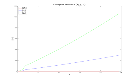
Figure 4.1: $\{(X_{k},y_{k},Z_{k})\}$ from Algorithm 3.1 typical behaviour; NO strict feasibility.

4.2 Jacobian Behaviour Near-Optimum and Degeneracy

In this section we study properties of the Jacobian of $F$ computed near an optimal point and relate its behaviour to the degeneracy status of the optimal point. In Section 4.2.1 we show that the degeneracy status of the optimal point characterizes the singularity of the Jacobian matrix. In Section 4.3 we study degeneracies of two classes of sets; the elliptope (the set of correlation matrices), and the vontope (feasible region of the SDP relaxation of the quadratic assignment problem, QAP). We exhibit the result from [39, Thm 3.4.2] that the elliptope has only nondegenerate points; however all vertices of the vontope are degenerate before FR, and some vertices of the vontope are degenerate even after FR.

4.2.1 Invertibility of Jacobian and Degeneracy

We extend the discussion of computing the Jacobian presented in Lemma 3.4 and elaborate the computational steps. Let $(\bar{X},\bar{y},\bar{Z})$ be an optimal triple that solves (3.3). We further assume that $\bar{X}$ and $\bar{Z}$ satisfy strict complementarity. Since $\bar{X}$ and $\bar{Z}$ are mutually orthogonally diagonalizable, we obtain

$$\bar{X}-\bar{Z}=W+{\mathcal{A}}^{*}(\bar{y})=\begin{bmatrix}V&\bar{V}\end{bmatrix}\begin{bmatrix}R&0\\ 0&-S\end{bmatrix}\begin{bmatrix}V&\bar{V}\end{bmatrix}^{T},\quad R\succ 0,\,S\succ 0,$$

where $\bar{X}=VRV^{T}$ and $\bar{Z}=\bar{V}S\bar{V}^{T}$.

Recall the steps for computing the Jacobian in Section 3.2.1. We now closely observe how the $(i,j)$-th element of the Jacobian in (3.11) is evaluated. Let $T_{j}$ be the matrix defined in (3.10). Then

$$\begin{array}[]{rcl}&&\tr(A_{i}\mathcal{R}_{\bar{X}}(T_{j}))\\ &=&\left\langle A_{i},\begin{bmatrix}V&\bar{V}\end{bmatrix}T_{j}\begin{bmatrix}V&\bar{V}\end{bmatrix}^{T}\right\rangle\\ &=&\left\langle\begin{bmatrix}V&\bar{V}\end{bmatrix}^{T}A_{i}\begin{bmatrix}V&\bar{V}\end{bmatrix},T_{j}\right\rangle\\ &=&\left\langle\begin{bmatrix}V^{T}A_{i}V&V^{T}A_{i}\bar{V}\\ \bar{V}^{T}A_{i}V&\bar{V}^{T}A_{i}\bar{V}\end{bmatrix},\begin{bmatrix}V^{T}A_{j}V&{\mathcal{B}}_{u}(\lambda(\bar{X}))\circ V^{T}A_{j}\bar{V}\\ \left({\mathcal{B}}_{u}(\lambda(\bar{X}))\circ V^{T}A_{j}\bar{V}\right)^{T}&0\end{bmatrix}\right\rangle\\ &=&\left\langle\begin{bmatrix}V^{T}A_{i}V&V^{T}A_{i}\bar{V}\\ \bar{V}^{T}A_{i}V&0\end{bmatrix},\begin{bmatrix}V^{T}A_{j}V&{\mathcal{B}}_{u}(\lambda(\bar{X}))\circ V^{T}A_{j}\bar{V}\\ \left({\mathcal{B}}_{u}(\lambda(\bar{X}))\circ V^{T}A_{j}\bar{V}\right)^{T}&0\end{bmatrix}\right\rangle.\end{array}$$ (4.3)

Note that the two arguments in the last trace inner product from (4.3) are identical up to the element-wise scaling. Lemma 4.5 below links the degeneracy of the optimal point $\bar{X}$ to the invertibility of the Jacobian at $\bar{X}$.

Lemma 4.5.

Let $D\in\mathbb{S}_{++}^{n}$ be a diagonal matrix, and let $\{x_{1},\ldots,x_{m}\}\subset\mathbb{R}^{n}$ be given. Let ${U}=\begin{bmatrix}x_{1}&x_{2}&\cdots&x_{m}\end{bmatrix}$. Then $\rank({U})=\rank({U}^{T}{U})=\rank({U}^{T}D{U})$.

Now we use (4.3), Lemma 4.5, and Lemma 2.12, to characterize the singularity of the Jacobian of $F$ evaluated at an optimal solution.

Theorem 4.6.

Let $\bar{X}$ be the optimal solution of the BAP (1.1). Then $\bar{X}$ is degenerate if, and only if, the Jacobian of $F$ at $\bar{X}$ is singular.

Proof.

Let $\bar{X}$ be the optimal point of (1.1). Let

$$D=\operatorname{{Diag}}\left(\operatorname{{svec}}\left(\begin{bmatrix}M&\frac{1}{\sqrt{2}}{\mathcal{B}}_{u}(\bar{X})\\ \frac{1}{\sqrt{2}}{\mathcal{B}}_{u}(\bar{X})^{T}&M\end{bmatrix}\right)\right)\in\mathbb{S}^{t(n)}_{++},$$

where $M=\frac{1}{\sqrt{2}}E+\left(1-\frac{1}{\sqrt{2}}\right)I$. Let $X_{i}:=\begin{bmatrix}V^{T}A_{i}V&V^{T}A_{i}\bar{V}\\ \bar{V}^{T}A_{i}V&0\end{bmatrix}$, and let $x_{i}:=\operatorname{{svec}}\left(X_{i}\right)$. We recall the definition of $T_{j}$ in (3.10) and note that

$$\operatorname{{svec}}\left(T_{j}\right)=Dx_{j}.$$

We then observe the last inner product in (4.3):

$$\left\langle X_{i},T_{j}\right\rangle=\left\langle\operatorname{{svec}}(X_{i}),\operatorname{{svec}}(T_{j})\right\rangle=\langle x_{i},Dx_{j}\rangle.$$

Now we form $U:=\begin{bmatrix}x_{1}&x_{2}&\cdots&x_{m}\end{bmatrix}\in\mathbb{R}^{t(n)\times m}$. Then, $\forall i,j$, we have

$$(U^{T}DU)_{i,j}=\left(\begin{bmatrix}x_{1}^{T}\\ \vdots\\ x_{m}^{T}\end{bmatrix}\begin{bmatrix}Dx_{1}\cdots Dx_{m}\end{bmatrix}\right)_{i,j}=x_{i}^{T}Dx_{j}=\tr(A_{i}\mathcal{R}_{\bar{X}}(T_{j})).$$

Therefore we conclude

$$\begin{array}[]{rcll}\bar{X}\text{ is degenerate }&\iff&\rank(U)<m&\text{by {(\ref{eq:RorateAis})}}\\ &\iff&U^{T}DU\text{ is singular }&\text{by \lx@cref{creftypecap~refnum}{lemma:JacodianReducedtoVec}}\\ &\iff&\text{Jacobian of $F$ at $\bar{X}$ is singular.}&\end{array}$$

 

Recall the sufficient conditions for producing a nondegenerate solution given in Propositions 2.18 and 2.17. Therefore, any projection point $\bar{X}$ that satisfies the conditions in Propositions 2.18 and 2.17 yields a nonsingular Jacobian.

4.3 Nondegeneracy of the Elliptope and Degeneracy of the Vontope

We now lead the discussion of degeneracy to the two classes of spectrahedra: the elliptope (the set of correlation matrices); and the vontope (the feasible set of the SDP relaxation of the quadratic assignment problem). For these two classes of problems, we illustrate how degeneracy interacts with the performance of Algorithm 3.1 in Section 5.2.

Example 4.7 (Elliptope, [47, Thm 3.4.2]).

We consider the problem of finding the nearest correlation matrix:

$$\min\left\{\frac{1}{2}\|X-W\|^{2}_{F}\,:\,\operatorname{{diag}}(X)=e,\,X\succeq 0\right\}.$$

The feasible region of the above problem is called the elliptope. Every point in the elliptope is nondegenerate.

Example 4.8 (Vontope, [49]).

Let $\Pi_{n}$ be the set of $n$-by-$n$ permutation matrices. For $X\in\Pi_{n}$, let

$$Y_{X}=y_{X}y_{X}^{T},\text{ where }y_{X}=\begin{pmatrix}1\cr\operatorname{{vec}}X\end{pmatrix}\in\mathbb{S}^{n^{2}+1}$$

be the lifted matrix. Here we index the rows and columns of a matrix starting from $0$. The lifting process gives rise to the following feasible region for the SDP relaxation:

$$\textit{${\mathcal{F}}_{\textbf{QAP}\,}$}:=\left\{Y\in\mathbb{S}^{n^{2}+1}_{+}:\begin{array}[]{l}G_{J}(Y)=E_{00},\operatorname{{b^{0}\operatorname{{diag}}}}(Y)=I_{n},\operatorname{{o^{0}\operatorname{{diag}}}}(Y)=I_{n},\\ Y_{0,j}=Y_{j,j},\forall j=1,\ldots,n^{2}+1\end{array}\right\}.$$ (4.4)

Here, $G_{J}$ is a linear map that chooses the elements in the index set $J$ that correspond to the off-diagonal elements of the $n$-by-$n$ diagonal blocks and the diagonal elements of the $n$-by-$n$ off-diagonal blocks; $\operatorname{{b^{0}\operatorname{{diag}}}}:\mathbb{S}^{n^{2}+1}\to\mathbb{S}^{n}$ and $\operatorname{{o^{0}\operatorname{{diag}}}}:\mathbb{S}^{n^{2}+1}\to\mathbb{S}^{n}$ are linear maps that sum the $n$-by-$n$ diagonal blocks and the $n$-by-$n$ off-diagonal blocks, respectively; see [49] for details on the construction of $G_{J},\operatorname{{b^{0}\operatorname{{diag}}}}$ and $\operatorname{{o^{0}\operatorname{{diag}}}}$. We remark that the expression in (4.4) contains redundant linear constraints.

It is well-known that the SDP relaxation of the QAP fails strict feasibility [49] and so we employ FR and work in a smaller space. Let

$$H=\begin{bmatrix}e^{T}\otimes I_{n}\cr I_{n}\otimes e^{T}\end{bmatrix}\in\mathbb{R}^{2n\times n^{2}},\ K=\begin{bmatrix}-e&H\end{bmatrix}\in\mathbb{R}^{2n\times(n^{2}+1)},$$

and let $\hat{V}\in\mathbb{R}^{(n^{2}+1)\times((n-1)^{2}+1)}$ be the matrix with orthonormal columns that spans $\operatorname{null}(K)$. FR leads to the following constraints:

$$\textit{${\mathcal{F}}^{\textbf{FR}\,}_{\textbf{QAP}\,}$}:=\{R\in\mathbb{S}^{(n-1)^{2}+1}:{\mathcal{G}}_{\hat{J}}(\hat{V}R\hat{V}^{T})=E_{00},\,R\succeq 0\},$$ (4.5)

where $G_{\hat{J}}$ a newly defined surjective linear map that chooses indices in $\hat{J}$ such that $\hat{J}\subsetneq J$. This aligns with the fact that FR reveals implicit redundant constraints. It is known that the number of equality constraints reduces to $n^{3}-2n^{2}+1$ after FR; see [49].

We now discuss the degeneracy of each lifted matrix $Y_{X}=y_{X}y_{X}^{T}=\hat{V}R_{X}\hat{V}^{T}$, $X\in\Pi_{n}$. Owing to the orthonormality of $\hat{V}$, we get

$$R_{X}=\hat{V}^{T}Y_{X}\hat{V}\in\mathbb{S}^{(n-1)^{2}+1}.$$

We note that $\rank(R_{X})=1$. We let $\{A_{i}\}_{i=1}^{n^{3}-2n^{2}+1}\subset\mathbb{S}^{(n-1)^{2}+1}$ be the set of matrices that realizes the affine constraints as the usual trace inner product. Hence the linear dependence of the matrices of the set (2.17) can be argued by their first columns; we observe that the vectors

$$\left\{\begin{pmatrix}V_{X}^{T}A_{i}V_{X}\\ \bar{V}_{X}^{T}A_{i}V_{X}\end{pmatrix}\right\}_{i=1}^{n^{3}-2n^{2}+1}\subseteq\mathbb{R}^{(n-1)^{2}+1},\quad{n^{3}-2n^{2}+1}>(n-1)^{2}+1,\ n\geq 3,$$

are linearly dependent, i.e., for $n\geq 3$. This proves that the rank-one vertices that arise from $\Pi_{n}$ are degenerate.

Remark 4.9.

If we replace $\mathbb{S}_{+}^{n}$ with $\mathbb{R}_{+}^{n}$, the set ${\mathcal{F}}$ reduces to a polyhedron and the discussion on the degeneracy simplifies. The degeneracy status of a point $x$ in a polyhedron can be confirmed by evaluating the rank of $A(:,\operatorname{{supp}}(x))$, where $\operatorname{{supp}}(x)$ denotes the support of $x$; see [47, Chapter 3]. The performance of the proposed algorithm in [10] is also affected by the degeneracy of the optimal point. Moreover every point of ${\mathcal{F}}$ as a polyhedron is degenerate in the absence of strict feasibility.

5 Numerical Experiments

To illustrate the effects on convergence and degeneracy, we now present multiple experiments using diverse spectahedra ${\mathcal{F}}$ with various ranges of values for the singularity degree, $\operatorname{sd}({\mathcal{F}})$, and for the implicit problem singularity, $\operatorname{{ips}}({\mathcal{F}})$. In our algorithm, dual feasibility and complementary slackness are satisfied exactly. Therefore, we use the following $\bm{\varepsilon}^{k}\in\mathbb{R}_{+}$ to denote the relative residual of the optimality conditions at iteration $k$:

$$\bm{\varepsilon}^{k}:=\min\left\{1,\frac{\|F(y^{k})\|}{1+\|b\|}\right\}=:\alpha_{k}10^{-t_{k}},\,1\leq\alpha_{k}<10.$$

We denote the condition number of the Jacobian of $F$ at $y^{k}$ as $\operatorname{{cond}}(J_{k})$, and let

$$\operatorname{{cond}}(J_{k})=\beta_{k}10^{s_{k}},\,1\leq\beta_{k}<10.$$

We stop Algorithm (3.1) once

$$(i)~{}~{}\bm{\varepsilon}^{k}\leq 10^{-13}\text{ or }(ii)~{}~{}s_{k}+t_{k}>16\text{ or }(iii)~{}~{}k>2000.$$

If condition (i) holds, then the we consider the BAP problem is solved. If condition (ii) holds, then we consider the optimal solution of the BAP problem as being degenerate. In our algorithm, if (ii) or (iii) hold, then we conclude that a small eigenvalue for the Jacobian exists and we assume that strict feasibility fails. And, by looking at the nonzero elements of an eigenvector associated to the smallest eigenvalue we get information on an exposing vector; and we identify constraints that give rise to the failure of strict feasibility. This solves an auxiliary system for a FR step, see Proposition 2.4. Using the information on the exposing vector, we then solve a reduced auxiliary system, using a Gauss–Newton approach. This results in a FR step. Following this, we remove the redundant constraints that arise from the FR step. We repeat until strict feasibility holds.

Numerical experiments are conducted with Matlab R2023b on a Windows 11 PC with Intel(R) Core(TM) i5-10210U CPU @ 1.60GHz, RAM 16.0GB.

5.1 Comparison With(out) Strict Feasibility

As expected, our tests in Table 5.1, show that Algorithm 3.1 performs exceptionally well for instances with strict feasibility but struggles when strict feasibility fails. In fact, we observe that Algorithm 3.1 achieves the relative precision of $10^{-7}$ in under $7$ iterations when strict feasibility holds. In contrast, when strict feasibility fails and Algorithm 3.1 converges, hundreds of iterations are needed to reach the desired precision. In Table 5.2, we repeat the same experiment setting a relative precision tolerance of $10^{-13}$ and allowing $2000$ iteration limit. Observe that, in this case, Algorithm 3.1 never reached the desired relative precision in under the maximum number of iterations when strict feasibility failed.

n	10	20	50	100
Slater	100%	100%	100%	100%
No Slater	55%	50%	50%	25%

Table 5.1: $20$ randomly generated problems 1.1; % converged $\bm{\varepsilon}^{k}\leq 10^{-8},k\leq 1000$.

n	10	20	50	100
Slater	100%	100%	100%	100%
No Slater	0%	0%	0%	0%

Table 5.2: $20$ randomly generated problems 1.1; % converged $\bm{\varepsilon}^{k}\leq 10^{-13},k\leq 2000$.

We now look at the case where the singularity degree $\operatorname{sd}({\mathcal{F}})=1$, while the implicit singularity $\operatorname{{ips}}({\mathcal{F}})$ varies.

5.1.1 $\operatorname{{ips}}({\mathcal{F}})=1$

We use a spectrahedra with singularity degree $1$ and $n=15,m=7$. The singularity degree is obtained by constructing an exposing vector as a linear combination of $5$ out of the $7$ constraints of the problem. Algorithm 3.1 is used to monitor the eigenvalues of the Jacobian of $F$ at every iteration $k$, see Figure 5.1. We observe that only one of the eigenvalues tends to $0$. After $452$ iterations the method reaches a relative residual of $9.9567\times 10^{-8}$, while the condition number of the Jacobian is $7.0236\times 10^{12}$. Therefore the algorithm stops and indicates which of the constraints are causing strict feasibility to fail. After applying FR and removing the single (implicit) redundant constraint found, the algorithm now succeeds and converges to a point with a relative residual of $1.0231\times 10^{-15}$ in only $8$ iterations, see Table 5.3.

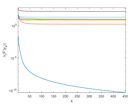
Figure 5.1: Changes in eigenvalues of Jacobian of $F$ for spectahedron in Section 5.1.1.

	$n$	$m$	$\bm{\varepsilon}^{k}$(rel. res.)	$\mathrm{cond}(F^{\prime}(y_{k}))$	$\lambda_{n}(y_{k})$	$k$
Before FR	15	7	9.9567e-08	7.0236e+12	-1.7238e-16	452
After FR	15	6	1.0231e-15	198.08	2.5515e-17	8

Table 5.3: spectahedron in Section 5.1.1; at final iteration $k$; before and after FR iters

5.1.2 $\operatorname{{ips}}({\mathcal{F}})>1$

In our second experiment, see Table 5.4, we work with data obtained from a SDP relaxation of the protein side-chain positioning problems, e.g., [9]. The spectahedra we are considering has singularity degree $1$, but the implicit problem singularity is greater than $1$, i.e., there are more than $1$ redundant constraints after applying FR . In particular, the dimension of the space is $n=35$ and the number of constraints is $m=75$. By running our algorithm, we observe that a large number of eigenvalues of the Jacobian tend to $0$ along the iterations (see Figure 5.2). After applying FR , we reduced the dimension of the problem to $n=10$ and the number of constraints to $m=22$. In the next run of the algorithm, only one eigenvalue of the Jacobian tends to $0$, but we detect that a second iteration of FR is needed. This time, we reduce $n$ to $9$ and we remove $6$ more redundant constraints, resulting in $m=16$. The next time we apply our algorithm, the method converges to the solution in $18$ iterations, see Table 5.4.

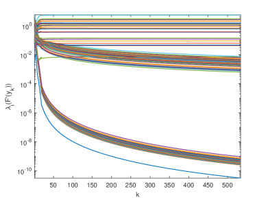
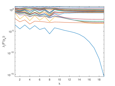
Figure 5.2: iterations $k$ vs eigenvalues; spectahedron in Section 5.1.2; before and after one FR iteration

	$n$	$m$	$\bm{\varepsilon}^{k}$(rel. res.)	$\mathrm{cond}(F^{\prime}(y_{k}))$	$\lambda_{n}(y_{k})$	$k$
Before FR	35	76	8.5351e-08	1.0060e+12	-1.6941e-15	534
After FR 1	10	22	7.6363e-04	1.8739e+16	-5.2097e-16	19
After FR 2	9	16	8.7202e-14	16103.37	-5.6900e-16	18

Table 5.4: spectahedron in Section 5.1.2; at final iteration $k$; before and after FR iters

5.2 Experiments with Elliptope and Vontope

In this section we address the importance of strict feasibility and degeneracy on the performance of Algorithm 3.1. We consider the elliptope and vontope cases. Furthermore we compare the performance of Algorithm 3.1 with the interior point solver SDPT3.

From Section 4.3 we recall that the MC problem satisfies strict feasibility and every point of the elliptope, the feasible set, is nondegenerate; see Example 4.7. The results from the MC problem are displayed in the line labelled ‘Elliptope’ in Table 5.5. As for the QAP, without FR, the SDP relaxation of QAP fails strict feasibility and all the feasible points are degenerate. Hence in our tests, we consider two models of the same set of instances: ${\mathcal{F}}_{\textbf{QAP}\,}$ obtained directly by the lifting of the variables (see (4.4)); and ${\mathcal{F}}^{\textbf{FR}\,}_{\textbf{QAP}\,}$ obtained after FR is applied to ${\mathcal{F}}_{\textbf{QAP}\,}$ (see (4.5)). In Table 5.5, QAP ($\textbf{QAP}_{\textbf{FR}}$, resp.) indicates the results obtained from ${\mathcal{F}}_{\textbf{QAP}\,}$ (${\mathcal{F}}^{\textbf{FR}}_{\textbf{QAP}}$, resp.).

We used two settings for the choice of $W$ in the objective function. The first setting for $W$ forces the optimal solution $\bar{X}$ to be rank $1$. Recall that rank-one optimal solutions for QAP  are degenerate and thus lead to ill-conditioned Jacobians as can be seen by the huge condition numbers in Table 5.5. The second setting chooses a random $W$.

For SDPT3 we provided the following second-order cone formulation of (1.1):

$$\min_{X,y,t}\left\{\ t\ :\operatorname{{svec}}(X)+y=\operatorname{{svec}}(W),\ ||y||_{2}\leq t,\ X\in{\mathcal{F}}\ \right\}.$$

The default settings for SDPT3 were used for the tests.

Each line of Table 5.5 reports on the average of $10$ instances, problem order $n=10$. The meaning of the header names used in Table 5.5 is as follows:

1. The headers pf, df and cs under Semi-Smooth Newton refer to the average of the primal feasibility, dual feasibility and complementarity, respectively, introduced in (2.11). The df includes both the linear dual feasibility and the violation of semidefiniteness. Both are essentially zero up to roundoff error of the arithmetic. Note that the values $e-15$ and smaller for pf and df are essentially zero (machine precision). The headers pf, df and cs under SPDT3 refer to the solver outputs, pinfeas, dinfeas and gap, respectively.

2. $k$ is the average number of iterations.

3. time is the average run time in cpu-seconds.

4. $\mathrm{cond}(F^{\prime}(y^{k}))$ is the average condition number of the Jacobian $(F^{\prime}(y^{k}))$; we only have this metric for the semi-smooth Newton method.

$W$ Generation	Problem	Semi-Smooth Newton						SDPT3
		pf	df	cs	$k$	time	$\mathrm{cond}(F^{\prime}(y^{k}))$	pf	df	cs	$k$	time
	Elliptope	9e-13	9e-16	2e-16	6.8	4e-02	3e+00	4e-12	6e-12	2e-07	15.5	2e-01
$W$, $\rank(\bar{X})=1$	$\textbf{QAP}_{\textbf{FR}\,}$	4e-07	2e-15	1e-16	7.5	7e+00	4e+15	5e-10	1e-09	9e-06	17.9	7e+01
	QAP	8e-09	3e-15	1e-16	8.6	2e+01	4e+14	5e-10	5e-09	1e-05	18.9	6e+01
	Elliptope	3e-12	1e-15	6e-17	6.3	1e-02	2e+00	1e-11	6e-12	3e-08	11.5	9e-02
random $W$	$\textbf{QAP}_{\textbf{FR}\,}$	2e-12	3e-15	7e-17	20.6	2e+01	3e+05	5e-10	5e-10	7e-07	13.9	5e+01
	QAP	1e-07	5e-13	3e-16	537.9	1e+03	6e+11	1e-08	2e-09	1e-06	17.3	7e+01

Table 5.5: Algorithm 3.1 and SDPT3 on: Elliptope and Vontope; $n=10$;

We now discuss the results in Table 5.5. We Start with the Semi-Smooth Newton, Algorithm 3.1. The pf column clearly shows that the degeneracy of the optimal point $\bar{X}$ plays an important role. Other than for random $W$ with $\textbf{QAP}_{\textbf{FR}}$, the pf values for the QAP problems are poor. This correlates with the condition number values; see also the discussion in Section 4. The condition numbers of the Jacobian near optimal points, $\operatorname{{cond}}(F^{\prime}(y^{k}))$, are ill-conditioned when strict feasibility fails and the optimal solution is degenerate. The good measures for df and cs of Semi-Smooth Newton method follow from the details of the construction of Algorithm 3.1.

SDPT3 displays an overall good performance on all instances, and this is typical for interior point methods. We note that the df and cs values under SDPT3 are weaker than for Semi-Smooth Newton due to the nature of interior point methods. The number of iterations is higher when the optimal solutions are set to be degenerate. The reason for the extremely high number of iterations for the case without FR is that a high accuracy is set but difficult to attain.

Algorithm 3.1 has a superior performance for MC problems as all components of the optimality conditions are satisfied with near machine accuracy. This confirms that the status of the optimal solution plays an important role when it comes to the performance of Algorithm 3.1. In addition, preprocessing the instances so that they satisfy strict feasibility is important as seen by problems failing strict feasibility only contain degenerate points; see Theorem 2.15.

6 Conclusions

We presented and analyzed a semi-smooth Newton method for the best approximation problem, the projection problem, for spectrahedra. We showed that nondegeneracy is needed for the semi-smooth Newton method to perform well. We used the unbounded dual optimal set in the absence of a regularity condition to explain the lack of good performance. Moreover, we showed that the absence of strict feasibility results in degeneracy and ill-conditioning of the Jacobian at optimality. Our empirics illustrate the importance of strict feasibility. In particular, we studied the degeneracy for the elliptope and vontope.

Though we concentrated on SDP, many current relaxations for hard problems involve the doubly nonnegative, DNN, cone, i.e., $\textbf{DNN}\,=\mathbb{S}_{+}^{n}\cap\mathbb{R}^{n\times n}_{+}$. In particular, splitting methods efficiently exploit this intersection of two cones and facial reduction often provides a natural efficient splitting, e.g., [36, 2, 22]. It seems that the results we obtained from the Newton method for the BAP would extend to applying splitting methods to feasible sets of the type ${\mathcal{L}}\cap\textbf{DNN}\,$.

6.1 Data Availability Statement

The results and data used in this paper is generated using our Matlab codes. These are publicly available at the link:
www.math.uwaterloo.ca%7EhwolkowihenryreportsCodesProjDegSingDegJul2024.d

6.2 Competing Interest Statement

Walaa M. Moursi is an associate editor of SVAA and is one of the authors of this paper. There is no other competing interest.

References

• [1] A. Alfakih, M. Anjos, V. Piccialli, and H. Wolkowicz, Euclidean distance matrices, semidefinite programming and sensor network localization, Port. Math., 68 (2011), pp. 53–102.
• [2] A. Alfakih, J. Cheng, W. L. Jung, W. M. Moursi, and H. Wolkowicz, Exact solutions for the np-hard Wasserstein barycenter problem using a doubly nonnegative relaxation and a splitting method, tech. rep., University of Waterloo, Waterloo, Ontario, 2023. 25 pages, research report.
• [3] A. Auslender and M. Teboulle, Asymptotic cones and functions in optimization and variational inequalities, Springer Monographs in Mathematics, Springer-Verlag, New York, 2003.
• [4] A. Barvinok, A remark on the rank of positive semidefinite matrices subject to affine constraints, Discrete Comput. Geom., 25 (2001), pp. 23–31.
• [5] H. Bauschke and V. Koch, Projection methods: Swiss army knives for solving feasibility and best approximation problems with halfspaces, in Infinite products of operators and their applications, vol. 636 of Contemp. Math., Amer. Math. Soc., Providence, RI, 2015, pp. 1–40.
• [6] R. Borsdorf and N. J. Higham, A preconditioned Newton algorithm for the nearest correlation matrix, IMA J. Numer. Anal., 30 (2010), pp. 94–107.
• [7] J. Borwein and H. Wolkowicz, Regularizing the abstract convex program, J. Math. Anal. Appl., 83 (1981), pp. 495–530.
• [8]  , A simple constraint qualification in infinite-dimensional programming, Math. Programming, 35 (1986), pp. 83–96.
• [9] F. Burkowski, H. Im, and H. Wolkowicz, A Peaceman-Rachford splitting method for the protein side-chain positioning problem, tech. rep., University of Waterloo, Waterloo, Ontario, 2022. arxiv.org/abs/2009.01450,21.
• [10] Y. Censor, , W. Moursi, T. Weames, and H. Wolkowicz, Regularized nonsmooth Newton algorithms for best approximation with applications, tech. rep., University of Waterloo, Waterloo, Ontario, 2022 submitted. 37 pages, research report.
• [11] Y. Censor, Weak and strong superiorization: between feasibility-seeking and minimization, An. Ştiinţ. Univ. “Ovidius” Constanţa Ser. Mat., 23 (2015), pp. 41–54.
• [12] M. de Carli Silva and L. Tunçel, Vertices of spectrahedra arising from the elliptope, the theta body, and their relatives, SIAM J. Optim., 25 (2015), pp. 295–316.
• [13] L. Ding and M. Udell, A strict complementarity approach to error bound and sensitivity of solution of conic programs, Optim. Lett., 17 (2023), pp. 1551–1574.
• [14] D. Drusvyatskiy, N. Krislock, Y.-L. C. Voronin, and H. Wolkowicz, Noisy Euclidean distance realization: robust facial reduction and the Pareto frontier, SIAM J. Optim., 27 (2017), pp. 2301–2331.
• [15] D. Drusvyatskiy, G. Li, and H. Wolkowicz, A note on alternating projections for ill-posed semidefinite feasibility problems, Math. Program., 162 (2017), pp. 537–548.
• [16] D. Drusvyatskiy and H. Wolkowicz, The many faces of degeneracy in conic optimization, Foundations and Trends® in Optimization, 3 (2017), pp. 77–170.
• [17] M. Dür, B. Jargalsaikhan, and G. Still, Genericity results in linear conic programming—a tour d’horizon, Math. Oper. Res., 42 (2017), pp. 77–94.
• [18] C. Eckart and G. Young, The approximation of one matrix by another of lower rank, Psychometrica, 1 (1936), pp. 211–218.
• [19] S. Friedland, Convex spectral functions, Linear and Multilinear Algebra, 9 (1980/81), pp. 299–316.
• [20] J. Gauvin, A necessary and sufficient regularity condition to have bounded multipliers in nonconvex programming, Math. Programming, 12 (1977), pp. 136–138.
• [21] P. Goulart, Y. Nakatsukasa, and N. Rontsis, Accuracy of approximate projection to the semidefinite cone, Linear Algebra and its Applications, 594 (2020), pp. 177–192.
• [22] N. Graham, H. Hu, H. Im, X. Li, and H. Wolkowicz, A restricted dual Peaceman-Rachford splitting method for a strengthened DNN relaxation for QAP, INFORMS J. Comput., 34 (2022), pp. 2125–2143.
• [23] D. Henrion and J. Malick, SDLS: a MATLAB package for solving conic least-squares problems, Tech. Rep. arXiv:0709.2556v1, LAAS,CVUT,LJK, 2007.
• [24] N. J. Higham, Computing the nearest correlation matrix—a problem from finance, IMA J. Numer. Anal., 22 (2002), pp. 329–343.
• [25] N. J. Higham and N. Strabić, Bounds for the distance to the nearest correlation matrix, SIAM J. Matrix Anal. Appl., 37 (2016), pp. 1088–1102.
• [26] H. Im, Implicit Loss of Surjectivity and Facial Reduction: Theory and Applications, PhD thesis, University of Waterloo, 2023.
• [27] H. Im, Implicit redundancy and degeneracy in conic program, tech. rep., arXiv, 2403.04171, 2024. arXiv, 2403.04171.
• [28] H. Im and H. Wolkowicz, A strengthened Barvinok-Pataki bound on SDP rank, Oper. Res. Lett., 49 (2021), pp. 837–841.
• [29]  , Revisiting degeneracy, strict feasibility, stability, in linear programming, European J. Oper. Res., 310 (2023), pp. 495–510. 35 pages, 10.48550/ARXIV.2203.02795.
• [30] A. Lewis, Convex analysis on the Hermitian matrices, SIAM J. Optim., 6 (1996), pp. 164–177.
• [31] J. Malick, A dual approach to semidefinite least-squares problems, SIAM J. Matrix Anal. Appl., 26 (2004), pp. 272–284 (electronic).
• [32] J. Malick and H. S. Sendov, Clarke generalized Jacobian of the projection onto the cone of positive semidefinite matrices, Set-Valued Anal., 14 (2006), pp. 273–293.
• [33] R. Mansour, New Algorithmic Structures for Feasibility-Seeking and for Best Approximation Problems and their Convergence Analyses, ProQuest LLC, Ann Arbor, MI, 2023. Thesis (Ph.D.)–University of Haifa (Israel).
• [34] C. Micchelli, P. Smith, J. Swetits, and J. Ward, Constrained $l_{p}$ approximation, Journal of Constructive Approximation, 1 (1985), pp. 93–102.
• [35] H. Ochiai, Y. Sekiguchi, and H. Waki, Analytic formulas for alternating projection sequences for the positive semidefinite cone and an application to convergence analysis, tech. rep., arXiv, 2024. 2401.15276, arXiv.
• [36] D. Oliveira, H. Wolkowicz, and Y. Xu, ADMM for the SDP relaxation of the QAP, Math. Program. Comput., 10 (2018), pp. 631–658.
• [37] N. Parikh and S. Boyd, Proximal algorithms, Foundations and Trends® in Optimization, 1 (2013), pp. 123–231.
• [38] G. Pataki, On the rank of extreme matrices in semidefinite programs and the multiplicity of optimal eigenvalues, Math. Oper. Res., 23 (1998), pp. 339–358.
• [39] G. Pataki, Geometry of Semidefinite Programming, in Handbook OF Semidefinite Programming: Theory, Algorithms, and Applications, H. Wolkowicz, R. Saigal, and L. Vandenberghe, eds., Kluwer Academic Publishers, Boston, MA, 2000.
• [40] M. Ramana, L. Tunçel, and H. Wolkowicz, Strong duality for semidefinite programming, SIAM J. Optim., 7 (1997), pp. 641–662.
• [41] S. Sremac, Error bounds and singularity degree in semidefinite programming, PhD thesis, University of Waterloo, 2019.
• [42] S. Sremac, H. Woerdeman, and H. Wolkowicz, Error bounds and singularity degree in semidefinite programming, SIAM J. Optim., 31 (2021), pp. 812–836.
• [43] J. Sturm, Error bounds for linear matrix inequalities, SIAM J. Optim., 10 (2000), pp. 1228–1248 (electronic).
• [44] D. Sun and J. Sun, Semismooth matrix-valued functions, Mathematics of Operations Research, 27 (2002), pp. 150–169.
• [45] K. Toh, M. Todd, and R. Tütüncü, SDPT3—a MATLAB software package for semidefinite programming, version 1.3, Optim. Methods Softw., 11/12 (1999), pp. 545–581. Interior point methods.
• [46] L. Tunçel and H. Wolkowicz, Strong duality and minimal representations for cone optimization, Comput. Optim. Appl., 53 (2012), pp. 619–648.
• [47] H. Wolkowicz, R. Saigal, and L. Vandenberghe, eds., Handbook of semidefinite programming, International Series in Operations Research & Management Science, 27, Kluwer Academic Publishers, Boston, MA, 2000. Theory, algorithms, and applications.
• [48] Y.-L. Yu, The proximity operator, in Semantic Scholar, 2014.
• [49] Q. Zhao, S. Karisch, F. Rendl, and H. Wolkowicz, Semidefinite programming relaxations for the quadratic assignment problem, J. Comb. Optim., 2 (1998), pp. 71–109. Semidefinite Programming and Interior-point Approaches for Combinatorial Optimization Problems (Fields Institute, Toronto, ON, 1996).