Enhanced Entanglement in Trion-Micropillars under Artificial Magnetic Fields

Abstract

We investigate quantum phenomena in a system of three coupled microcavities each supporting regime of strong coupling with exciton resonance. The possibility of observing polariton blockade in a dimer and triple micropillar configuration is discussed. We identify the resonance conditions corresponding to the onset of the photon blockade. The discovered quantum effects allow using these systems as versatile sources of individual polaritons. Various manifestations of the quantum blockade can be tuned with the use of the pumping laser frequency. We demonstrate that the presence of the cascade coupling between pillars enhances manifestations of sub-Poissonian statistics. Application of the effective gauge field in the triangle configuration allows for manifestation of a collective antibunching effect. In particular, we identify conditions of a multimode blockade – a phenomenon consisting in blocking of excitation of the state with $n$ particles distributed over multiple coupled modes. A new effect of quantum entanglement of a non-Hermitian dimer with a micropillar in an artificial magnetic field has been discovered, associated with the simultaneous manifestation of antibunching on the dimer, the micropillar associated with it, and the triple-micropillar.

I introduction

Quantum correlations reflect the non-classical nature of quantum states - the impossibility of representing the whole as a sum (Cartesian product) of its parts. Many-particle interactions in multimode bosonic systems provide an opportunity to implement quantum topological materials [1, 2] and multimode entanglement [3]. Multimode photon blockade can be utilized to execute universal operations on qubits and qudits in various bosonic modes within coupled microcavity systems [4]. Qubits in coupled micropillar system are realized on top of exciton-polariton condensates by utilizing quantum weak perturbation of the mean-field value [5]. The exploration of the quantum statistical properties of nonlinear light-matter systems is highly valuable due to its applications in the field of quantum information [6, 7, 5] and the development of single-photon sources [8, 9, 10, 11].

The quantum nature of light is reflected in its statistical properties such as sub-Poisson statistics and in the violation of classical inequalities (of Cauchy-Schwartz type) on correlation functions. The interaction of a photon with a nonlinear system prevents interaction with further photons, resulting in the emission of a single photon. This effect allows systems to suppress the emission of photons in the form of pairs ($g^{(2)}(0)=0$), and lead to sub-Poissonian statistic of radiation [12]. This is an effect of photon blockade [10, 16, 13, 15, 14] that allows the conversion of coherent laser light into a stream of individual photons in the Fock state [17], when autocorrelations arise in the photon count. The quantum anticorrelations of the radiation emitted by the nonlinear systems typically originates from the spectrum anharmonicity [10, 18]. The anharmonicity leads to the fact that the first excited state of an oscillator is not resonant with the second excited state. So, the appearance of two photons at the same frequency is unlikely (but becomes possible in the presence of the dissipation-induced broadening). Usually, a pronounced photon blockade effect requires an inter-particle interaction strength $U$ comparable to the net loss rate $\gamma$. In contrast, the unconventional photon blockade (UPB) can occur in weakly nonlinear systems with $U<\gamma$, which is a typical condition in condensed matter physics [16, 19, 20, 21]. To maintain stationary population of optical modes, resonators are usually used. A typical system for studying interaction of light and matter is low-dimensional systems - quantum wells [22] or quantum dots [23] embedded in a microcavity.

Semiconductor Bragg resonators can concentrate optical radiation in a small volume on a micrometers scale [24]. These structures also have high $Q$-factors, allowing for a control of a photon signal unattainable in other types of resonators. They are manufactured using molecular beam epitaxy, with flat resonators being the most popular configuration, resembling a quantum well between two Bragg mirrors [25]. Chemical etching enables control over the resonator’s shape. This approach achieves high optical radiation concentration in the in-plane direction. An example is resonators with circular cross-section, which are microscopic columns - pillar microcavities (MP) [26, 27, 28, 29] with typical for this system weak nonlinearity [30] $U\approx 0.01\gamma$. Such micropillar systems enable creation of highly bright sources of single photons with $g^{(2)}$ reaching $0.05$ [31, 32]. The sub-Poisson statistics of radiation from MPs, including those supporting strong coupling between exciton and photon modes, was predicted theoretically for weak [33, 34] and strong pumping [35].

The physical basis for studying many-body interactions can be arrays of micropillars interacting through tunneling photons arranged in a graph configuration and described by the Bose-Hubbard model on such a graph. The topological properties of such systems were studied in the works [37, 36]. It is known that cyclic connections in the graph violate gauge invariance to the artificial magnetic field [38]. In this work, a triangle of micropillars is considered and its non-trivial statistical properties are investigated.

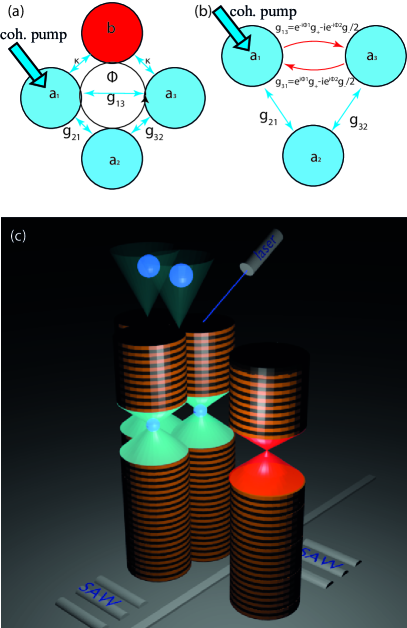
Figure 1: (a) A sketch of a polariton quadruplet which can be reduced to the non-reciprocal triple-micropillar (see appendix C) by adiabatic elimination of a rapidly decaying mode $b$ (empty MP, i.e. having no active medium). (b) Sketch of a triangular connection diagram of MP with Hermitian coupling; (c) Schematic sample design of non-hermitain trion+empty MP. The device consists of an trion MPs with cavity are excited via laser and modulated cavity of MP use surface acoustic wave (SAW).

The article has the following structure: in the first section, a general model of a polariton trion see 1b consisted of three closely placed MPs is introduced. In the second section, we consider the statistics of the polariton dimer, and then move on to the section devoted to the polariton triple-micropillar. Third section obtain condition for multimode quantum blockade for the polariton triple-micropillar.

II Model

Consider the following model of four tunnel-connected [39] micropillars (MPs) see fig.1(a) which are modeled as four non-linear quantum oscillators in the presence of a drive field of the following form (in the rotating wave approximation):

$$\begin{array}[]{l}{\hat{H}=\sum_{i=1}^{3}\Delta_{i}\hat{a}^{{\dagger}}_{i}\hat{a}_{i}+\sum_{i\neq j}^{3}g_{ij}\hat{a}^{{\dagger}}_{i}\hat{a}_{j}}+\\ +{\sum_{i=1}^{3}F_{i}(\hat{a}_{i}^{{\dagger}}+\hat{a}_{i})+U_{i}\hat{a}^{{\dagger}}_{i}\hat{a}^{{\dagger}}_{i}\hat{a}_{i}\hat{a}_{i}}+\\ +{(\omega_{b}-\omega_{L})\hat{b}^{{\dagger}}\hat{b}+\kappa(\hat{a}_{1}^{{\dagger}}+\hat{a}_{2}^{{\dagger}})\hat{b}+\kappa\hat{b}^{{\dagger}}(\hat{a}_{1}+\hat{a}_{2})},\end{array}$$ (1)

Here $\hat{a}_{i}$($\hat{a}_{i}^{{\dagger}}$) being a polariton annihilation (creation) operator (Bose) in the $i^{\rm th}$ MP while $U_{i}$ quantifies the strength of the interparticle interaction inside the $i^{\rm th}$ MP [40]; $\Delta_{i}=\omega_{i}-\omega_{L}$ is the detuning of the $i^{\rm th}$ cavity from the frequency $\omega_{L}$ of the coherent driving field $F_{i}$ which is injected into $i^{\rm th}$ MP, $g_{ij}$ is the coupling amplitude between $i^{\rm th}$ and $j^{\rm th}$ MPs.

For the description of the open quantum system we use a general master equation for the density matrix:

$$\begin{array}[]{l}i\frac{\partial\rho}{\partial t}=\left[\hat{H},\rho\right]+i\sum_{j=1}^{3}{\gamma_{j}\mathbf{D}[\hat{a}_{j};\rho]}+i\gamma_{b}\mathbf{D}[\hat{b};\rho]\end{array},$$ (2)

where we define the dissipator super-operator $\mathbf{D}[a;\rho]=\hat{a}\rho\hat{a}^{{\dagger}}-\frac{1}{2}\{\hat{a}^{{\dagger}}\hat{a},\rho\}$ which describes interaction with the environment with the rates $\gamma_{1,2,3}$ for the first three MPs and $\gamma_{b}>\gamma_{1,2,3}$ - is the dissipation parameter of the fourth MP $"b"$. Here $\{.,.\}$ stands for the anticommutator.

Adiabatically eliminating empty fast decay MP $"b"$ [38], – see appendix A, we obtain an effective the triple-micropillar system shown in Fig. 1b with the following non-Hermitain Hamiltonian:

$$\begin{array}[]{l}{\hat{H}_{t}=\mathbf{\hat{a}^{{\dagger}}}\mathbf{G}\mathbf{\hat{a}}+F_{1}(\hat{a}_{1}^{{\dagger}}+\hat{a}_{1})+\sum_{i}{U_{i}\hat{a}^{{\dagger}}_{i}\hat{a}^{{\dagger}}_{i}\hat{a}_{i}\hat{a}_{i}}},\end{array}$$ (3)

Here $\mathbf{\hat{a}}=\left(\hat{a}_{1},\hat{a}_{2},\hat{a}_{3}\right)^{\intercal}$, $\mathbf{\hat{a}^{{\dagger}}}=\left(\hat{a}_{1}^{{\dagger}},\hat{a}_{2}^{{\dagger}},\hat{a}_{3}^{{\dagger}}\right)^{\intercal}$ is a vector of annihilation and creation operators.

The following matrix was introduced in (3):

$$\mathbf{G}=\begin{bmatrix}\Delta_{1}&g_{12}&e^{-i\Phi_{1}}g_{+}-\frac{i}{2}e^{-i\Phi_{2}}g_{-}\\ g_{21}&\Delta_{2}&g_{23}\\ e^{i\Phi_{1}}g_{+}-\frac{i}{2}e^{i\Phi_{2}}g_{-}&g_{32}&\Delta_{3}\end{bmatrix},$$ (4)

where $g_{\pm}$ – are Hermitian and non-Hermitian coupling strength, see appendix A.

We can rewrite master equation (2) as:

$$\begin{array}[]{l}i\frac{\partial\rho}{\partial t}=\left[\hat{H}_{t}^{+},\rho\right]+\{\hat{H}_{t}^{-},\rho\}+i\sum_{j=1}^{3}{\gamma_{j}D[\hat{a}_{j}]}+ig_{d}D[\hat{a}_{1}+\hat{a}_{3}]\end{array},$$ (5)

where $\hat{H}_{t}^{\pm}$ are the Hermitian and non-Hermitian parts of the full Hamiltonian (3), see appendix A.

The concept of representing the field as a collection of interconnected ”balls”, using a connectivity matrix to describe their coupling coefficients, and incorporating a deformation tensor to account for changes in these couplings, provides a framework for understanding the dynamic nature of field interactions. In the context of the general theory of relativity, space-time is characterized by curvature, a product of the mass and energy distribution within it. This curvature caused by the mass and energy distribution can lead to the generation of magnetic fields through the motion of charged particles.

The consideration of three coupled oscillators as the simplest configuration stems from its gauge invariance with respect to an artificially introduced magnetic field [38]. This artificial magnetic field is introduced in (4) via an invariant phases $\Phi_{1},\Phi_{2}$ in the coupling strength, as detailed in appendix B. The two circuits give two invariant phases, see Appendix C, but it can be shown, see Appendix C, that these two phases can be reduced to a single phase $\Phi(\Phi_{1},\Phi_{2})$. This phases can be obtained surface acoustic wave modulated eignfrequency of MPs [41], see fig.1(c).

The master equation (5) is the most accurate description of quantum processes of quantum systems separated from their environment. However, if we neglect quantum jumps $a_{i}\rho a_{j}^{{\dagger}}$ (where $i,j=1,2,3$ and $i\neq j$), we can rewrite the matrix (4):

$$\mathbf{G_{eff}}=\begin{bmatrix}\tilde{\Delta_{1}}&g_{12}&(e^{-i\Phi_{1}}g_{+}-\frac{i}{2}e^{-i\Phi_{2}}g_{-})\\ g_{21}&\tilde{\Delta_{2}}&g_{23}\\ (e^{i\Phi_{1}}g_{+}-\frac{i}{2}e^{i\Phi_{2}}g_{-})&g_{32}&\tilde{\Delta_{3}}\end{bmatrix},$$ (6)

here we take in account non-Hermicity through changing settings to the complex manifold $\Delta_{i}\Rightarrow\tilde{\Delta_{1,3}}=\Delta_{1,3}-i\gamma_{1,3}/2-ig_{-}/2,\tilde{\Delta_{2}}=\Delta_{2}-i\gamma_{2}/2$.

The we rewrite the Hamiltonian (3) using (6):

$$\begin{array}[]{l}{\hat{H}_{eff}=\mathbf{\hat{a}^{{\dagger}}}\mathbf{G_{eff}}\mathbf{\hat{a}}+\sum_{i}{F_{i}(\hat{a}_{i}^{{\dagger}}+\hat{a}_{i})}+\sum_{i}{U_{i}\hat{a}^{{\dagger}}_{i}\hat{a}^{{\dagger}}_{i}\hat{a}_{i}\hat{a}_{i}}}\end{array}.$$ (7)

The corresponding wave function of the system can be written as a ket vector in the Fock-space basis:

$$|\psi\rangle=\sum_{i+j+k<=M}c_{ijk}(t)|ijk\rangle,$$ (8)

where $M$ is a size of the truncated Hilbert space which corresponds to the maximum number of photons in the system. This function is governed by the Schrödinger equation

$$i\frac{d}{dt}|\psi\rangle=H_{eff}|\psi\rangle,$$ (9)

which obeys the matrix elements to satisfy the following equations

$$\begin{array}[]{l}{\frac{idc_{ijk}}{dt}=\sum_{l}(\Delta_{l}n_{l}+U_{l}n_{l}(n_{l}-1))c_{ijk}+}\\ {+F_{1}\sqrt{n_{1}+1}c_{(i+1)jk}+F_{2}\sqrt{n_{1}}c_{(i-1)jk}+}\\ {+g_{12}\sqrt{n_{1}(n_{2}+1)}c_{(i-1)(j+1)k}+g_{21}\sqrt{n_{2}(n_{1}+1)}c_{(i+1)(j-1)k}+}\\ {+g_{13}\sqrt{n_{1}(n_{3}+1)}c_{(i-1)j(k+1)}+g_{31}\sqrt{n_{2}(n_{1}+1)}c_{(i+1)j(k-1)}+}\\ {+g_{23}\sqrt{n_{2}(n_{3}+1)}c_{i(j-1)(k+1)}+g_{32}\sqrt{n_{3}(n_{2}+1)}c_{i(j+1)(k-1)}}.\end{array}$$ (10)

Here $c_{ijk}$ - the amplitude of the probability of the system being in one of the states $|i,j,k>$.

We can rewrite Eq. (10) as a sum of $n-$particles states [42]:

$$|\psi\rangle=\sum_{n<=M}|\psi^{(n)}\rangle,$$ (11)

here we introduce state with $n$-particle quantum state:

$$|\psi^{(n)}\rangle=\sum_{i+j+k=n}c_{ijk}|ijk\rangle,$$ (12)

where $i+j+k=n$ is total number of particles in the state $|ijk\rangle$, which denotes a state with $i$ particles in the first mode, $j$ particles in the second mode and $k$ particles in the third mode.

Rewrite the effective Hamiltonian (7) as a block-matrix consistent from $n$-particle Hamiltonians as (see appendix C)

$$H_{eff}\approx\mathbf{\hat{a}^{{\dagger}}}diag(G_{eff},G^{(2)},...,G^{(n)})\mathbf{\hat{a}}+\sum_{i}{F_{i}\hat{a}_{i}^{{\dagger}}}$$ (13)

the notation $diag(a_{1},a_{2},...)$ represents a diagonal matrix using the provided elements $a_{1},a_{2},...$ and so on. The first part of the Hamiltonian is a block one and consists of Hamiltonians acting on $n$-particle states with matrices $G^{(n)}$ with rank n(1+n)/2, these can be represented as tensor networks of a certain rank. The second part of the Hamiltonian takes the system from a lower rank tensor network to a higher one.

The non-classical effects can be detected by measuring the second (or higher) order correlation or cross-correlation functions. The second-order correlation function for the $i^{\rm th}$ microcavity is defined as:

$$\begin{array}[]{l}{{g^{\left(2\right)}_{i}\left(0\right)=\frac{\left\langle\hat{a}^{{\dagger}2}_{i}\hat{a}^{2}_{i}\right\rangle}{\left\langle\hat{a}^{{\dagger}}_{i}\hat{a}_{i}\right\rangle^{2}}}}\end{array}.$$ (14)

III Methods

The task was to find the optimal parameters when the blockade effect occurs. To do this, the stationary Schrödinger equation with the effective Hamiltonian $\eqref{Eq15_}$ was solved, see Appendix C. Next, the master equation $\eqref{Eq5_}$ was solved numerically using the QuTiP package version 4.7.1, a Quantum Toolbox in Python [43] with the found parameters. Codes are available upon request by email thomasheisenberg@mail.ru.

IV Results

IV.1 Dimer

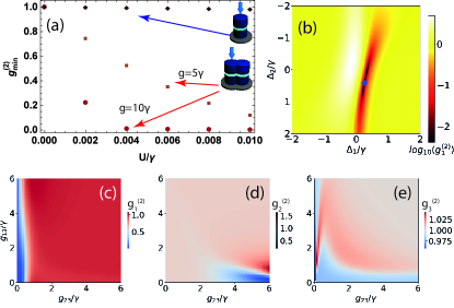
Figure 2: (a) The minimum value of the second order correlation function for the first micropillar (which are pump) $g^{(2)}_{2}$ for different values of the coupling amplitude: blue squared – two coupled micropillars with the coupling constant $g=5\gamma$ and the green dots with the coupling amplitude $g=10\gamma$ and red diamonds denote one micropillar. Other parameters are: [44]: $U_{1}=U_{2}=U_{3}=U_{LP}=0.01\gamma_{1},\gamma_{1}=\gamma_{2}=\gamma_{3}=\gamma,F_{1}=\gamma_{1},F_{2}=0,F_{3}=0,\hbar\gamma=0.0274$ meV. (b) The $g^{2}_{1}$ - correlation function map for the first micropillar. The blue disk (with coordinates $\Delta_{1}/\gamma=0.3,\Delta_{2}/\gamma=0.1$) on the map corresponds to the minimum value of the function $g^{(2)}_{1}$ for the optimal coupling constant $g=6.2\gamma$ obtained using (15). (c-e) The $g^{(2)}$-correlation function map for the first, second and third micropillars for Hermitian triple micropillar as functions of the coupling amplitudes between the second and the third micropillars for parameters (c-e panels) $\Delta_{1}/\gamma=0.4,\Delta_{2}/\gamma=0.3,\Delta_{3}/\gamma=0.4,F_{1}=0.1\gamma,F_{2,3}=0,g_{12}=g_{21}=5\gamma$.

With a dimer, sub-Poissonian statistics can be observed at small nonlinearities via unconventional scenario while a single pillar exhibits only weakly non-classical behavior, see fig.2a in this regime. The optimal conditions for the minimum $g^{(2)}_{1}$ have been found; for the quantum blockade regime, see fig. 2b.

For a dimer the conditions of quantum blockade by coupling [21] (for resonance condition):

$$g_{opt}/\gamma\approx\sqrt{\frac{2}{27}}\sqrt{\sqrt{3+4\left(\frac{U}{\gamma}\right)^{2}}\left(\frac{U}{\gamma}+3\frac{\gamma}{U}\right)-2\left(\frac{U}{\gamma}\right)^{2}}$$ (15)

When the third micropillar is connected to the dimer, the antibunching effect observed on the first micropillar remains relatively constant and shows a weak correlation with the connection strength $g_{13}$ between the first and third micropillars (Fig. 2c). However, when the connection strength $g_{23}$ between the second and third micropillars is increased, the antibunching effect vanishes, as illustrated in Fig.2c. In such a scenario, the statistics for the second micropillar, with a strong coupling represented by $g_{23}$, exhibit non-classical behavior with the onset of the antibunching effect shown in Fig. 2d. The antibunching effect transitions to the second micropillar as the connection with the third micropillar is enhanced, while there is minimal impact on the statistical behavior of the third micropillar, as depicted in Fig. 2e. By introducing the third micropillar, additional pathways for quantum blockade interference are established, enabling quantum destructive interference with the blockade of higher states - a phenomenon that is exclusive to the micropillar under excitation. Notably, if both coupling parameters $g_{13}$ and $g_{23}$ are simultaneously increased, the antibunching effect disappears.

IV.2 Trion

Analysis of the quantum statistics of the Hermitian triple micropillar revealed the disappearance of the effect of quantum blockade. In $PT$-symmetry non-Hermitian system, the quantum blocked effects within use non-reciprocal coupling were discovered [45]. For obtained non-reciprocal coupling, we added a fourth fast-decaying micropillar $\gamma_{b}>\gamma_{i}$ without a quantum dot coupled with fist and third MPs with a coupling coefficient $~{}\kappa$, see Fig.1a. Then this MP was adiabatically excluded, see Appendix A, and an effective nonlinear three-mode system was obtained - a triple micropillar with non-Hermitain coupling between the first and the third MPs with Hamiltonian (3).

When we do not distinguish from which MP the photon came (assuming equal radiation frequencies), we can consider three or two MPs as a single source of photons, wherein the optical mode’s radiation pattern should remain consistent regardless of polarization, so as to prevent any ’which-path’ information are obtained from angle radiation [46].

If someone blocks the signal from any micropillar, the radiation statistics of a collective emission of the triple micropillar changes significantly. The output mixed second order for the first and the third MPs (non-reciprocal polariton dimer) is defined as:

$$\begin{array}[]{l}{g_{1+3}^{\left(2\right)}(0)=\frac{\left\langle\hat{a}_{1+3}^{{\dagger}2}\hat{a}_{1+3}^{2}\right\rangle}{\left\langle\hat{a}_{1+3}^{{\dagger}}\hat{a}_{1+3}\right\rangle^{2}}\approx}\\ {\approx 2\mathcal{N}\frac{|c_{200}+c_{002}+\sqrt{2}c_{101}|^{2}}{|c_{100}+c_{001}|^{4}}}\end{array}$$ (16)

This way, the output mixed second order for the signal from the whole triple-micropillar structure is:

$$\begin{array}[]{l}{g_{1+2+3}^{\left(2\right)}(0)=\frac{\left\langle\hat{a}_{1+2+3}^{{\dagger}2}\hat{a}_{1+2+3}^{2}\right\rangle}{\left\langle\hat{a}_{1+2+3}^{{\dagger}}\hat{a}_{1+2+3}\right\rangle^{2}}\approx}\\ {\approx 2\mathcal{N}\frac{|c_{200}+\sqrt{2}c_{110}+c_{020}+\sqrt{2}c_{101}+c_{002}+\sqrt{2}c_{011}|^{2}}{|c_{100}+c_{010}+c_{001}|^{4}}}\end{array}$$ (17)

where $\mathcal{N}=\sum_{n=0}^{M}{\sum_{i+j+k=n}{|c_{ijk}^{(n)}|^{2}}}$ - is normalization constant. Also we introduced the following notation $a_{\sum{i}}=\sum{a_{i}}$ is the collective output mode subspace of the multimode space state [47]. Also here the approximation of the truncated wave function (11) on two particles is used.

We find the following optimal parameters from steady state solution (9) with effective Hamiltonian (13): $\gamma=0.1ps^{-1},\gamma_{1}=0.128\gamma,\gamma_{2}=\gamma,\gamma_{3}=0.28\gamma,U_{1}=U_{2}=U_{3}=0.01\gamma,F_{1}=0.1\gamma,F_{2}=0,F_{3}=0,g_{12}=g_{21}=g_{23}=g_{32}=g=0.39\gamma,g_{+}=4.86\gamma,g_{-}=4.97\gamma$ and $\Phi_{1}=7\pi/20,\Phi_{2}=7\pi/10,\Delta_{1,2,3}=\Delta=0$.

Radiation from whole triple micropillar is almost coherent $g_{1+2+3}^{(2)}(0)=0.969$. However, if we block the light from the second micropillar which is connected to the non-reciprocal polariton dimer, then the radiation from the triple micropillar becomes more ordered than the coherent radiation. An antibunching effect will occur with minimum value $g_{1+3}^{(2)}(0)=0.058$. Figure 3a,b demonstrate this correlation functions in the dependency of the detuning $\Delta$. Note that for individual MPs $g_{1,2}^{(2)}(0)\approx 1$, $g_{3}^{(2)}(0)\approx 0.8$.

Let’s adjust the pump frequency by $\Delta_{1,2,3}=1.8\gamma$ and find the phases values $\Phi_{1}=9\pi/20,\Phi_{2}=11\pi/10$. Then we have ${g^{(2)}_{1+2+3}}_{min}=0.057$,${g^{(2)}_{1+3}}_{min}=0.202$. How the correlation functions change for this case are shown in the figures 3c,d. Let’s adjust the pump frequency by $\Delta_{1,2,3}=1.8\gamma$ and find the phase values $\Phi_{1}=9\pi/20,\Phi_{2}=11\pi/10$. Then we have antibunching for full triple micropillar ${g^{(2)}_{1+2+3}}_{min}=0.057$ and ${g^{(2)}_{1+3}}_{min}=$0.202. Changes in the correlation functions when varying the detuning from the optimal value are shown in Figures 3c, d.

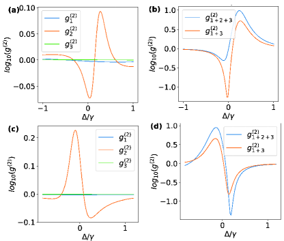
Figure 3: (a,c) Correlation characteristics for individual MPs, (b,d) mixed correlation function $\eqref{Eq16a_}$,$\eqref{Eq16b_}$ of $\Delta$. Parameters are: $\gamma=0.1ps^{-1},\gamma_{1}=0.128\gamma,\gamma_{2}=\gamma,\gamma_{3}=0.28\gamma,U_{1}=U_{2}=U_{3}=0.01\gamma,F_{1}=0.1\gamma,F_{2}=0,F_{3}=0,g_{12}=g_{21}=g_{23}=g_{32}=g=0.39\gamma,g_{+}=4.86\gamma,g_{-}=4.97\gamma$ (a,b) $\Phi_{1}=7\pi/20,\Phi_{2}=7\pi/10$ and (c,d) $\Phi_{1}=9\pi/20,\Phi_{2}=11\pi/10$. These results were obtained from the solution of the master equation (5) using the QuTiP package version 4.7.1, a Quantum Toolbox in Python [43].

The conditions for multimode blockade are achieved if the sum of the amplitudes of the corresponding probabilities is equal to zero, otherwise if the amplitudes are represented as vectors, then the blockade condition is reduced to the condition of the closedness of the polygon of state vectors, see Fig. 4c.

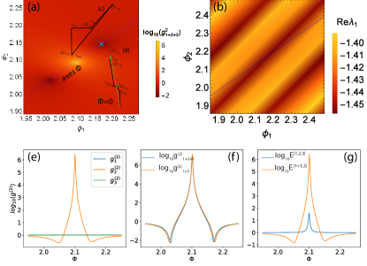
Figure 4: (a). The heat map of output mixed second order for the signal from the whole triple-micropillar structure in dependency artificial magnetic fields $\phi_{1,2}$; (b) first eigenvalue of matrix $G^{(2)}$; (c) Graphic representation of the summation amplitude of probability for blockade case (blue cross on panel (a)) and (d) not collective blockade $\Phi=0$; (e) The second order correlation function for each MP; (f) The output mixed second order correlation function from whole structure and non-hermitian coupled MP depending on the magnetic field $\Phi(\phi_{1},\phi_{2})=k\phi_{2}+b$ along the dashed line in panel (a), here $k=0.69,b=0.67$; (g) Entanglement criterion. Parameters are: $g_{+}=g_{-}=5\gamma,g=0.4\gamma,\Delta=-4.76\gamma$.

Quantum blockade of the sum mode of a triple micropillar occurs in the presence of an artificial magnetic field, while in the non-Hermitian triple micropillar there are two phases (see Appendix C), the effects of bunching and antibunching appear along the dashed line shown $\Phi(\phi_{1},\phi_{2}),$see fig. 4a, it passes at an angle to the spectrum of the matrix $G^{(2)}$, see fig. 4b. In this magnetic field, a region with a giant bunching effect appears, on both sides of which there are two regions with a strong antibunching effect with $g^{(2)}_{1+2+3}=0.006$.

For the polariton blockade effect to occur, it is necessary that the probability amplitudes of two-particle (with certain multipliers) states add up to zero, i.e. If you imagine this graphically, they were closed, see fig. 4c. In particular, if, with these parameters, the phase is removed from the Hermitian coupling, then there will be no short circuit - see the green arrow on fig. 4d.

When blockade is simultaneously present on the triple-micropillar fig. 4f on a non-Hermitian dimer fig. 4f and antibunching is observed on the second micropillar fig. 4e (attached), then quantum entanglement between the dimer and the micropillar is observed in the system, while there is no three-mode quantum entanglement throughout the entire triple-micropillar, see fig. 4g.

We can use Hillery-Zubairi two mode entanglement criteria [47, 48] for one mode ”2” and sum mode ”1+3”:

$$E^{(1+3,2)}=\frac{\left\langle(\hat{a}_{1}^{{\dagger}}+\hat{a}_{3}^{{\dagger}})(\hat{a}_{1}+\hat{a}_{3})\hat{a}_{2}^{{\dagger}}\hat{a}_{2}\right\rangle}{|\left\langle\hat{a}_{2}^{{\dagger}}(\hat{a}_{1}+\hat{a}_{3})\right\rangle|^{2}}\stackrel{{\scriptstyle\text{ent}}}{{<}}1,$$ (18)

and for three mode [47, 48]:

$$E^{(1,2,3)}=\frac{\langle\hat{a}_{1}^{{\dagger}}\hat{a}_{1}\hat{a}_{2}^{{\dagger}}\hat{a}_{2}\hat{a}_{3}^{{\dagger}}\hat{a}_{3}\rangle}{|\langle a_{1}^{{\dagger}}a_{2}a_{3}\rangle|^{2}}\stackrel{{\scriptstyle\text{ent}}}{{<}}1$$ (19)

Let us present simple considerations of the connection between quantum blockade of collective modes and quantum entanglement, with simultaneous blockade on the entire trion and on the non-Hermitian dimer, we obtain from the numerator $\eqref{Eq16b_}$ that $c_{020}+\sqrt{2}(c_{110}+c_{011})\approx 0$, and since $E^{(1+3,2)}\sim|c_{110}+c_{011}|^{2}$, then if $c_{020}\approx 0$, therefore $c_{110}+c_{011}\approx 0$ and numerator of $E^{(1+3,2)}\approx 0$.

V Conclusion

The study demonstrates that quantum blockade occurs of the sum mode of a triple micropillar in the presence of an artificial magnetic field, and the effects of bunching and antibunching are observed along a specific magnetic line. For the polariton blockade effect to manifest, it is necessary for the probability amplitudes of two-particle states to sum to zero, and quantum entanglement is observed between the dimer and the micropillar while being absent in the three-mode entanglement not have. It is known that for indistinguishable bosons, the probability of occupying a single state increases with the population. Interparticle interactions can prevent such population and lead to the effect of quantum unconventional blockade. Unlike the Pauli exclusion principle (which are fundamental law), such blockade occurs only under certain conditions of system parameters. The study identified conditions under which multimode blockade is observed in several micropillars connected in a triangular configuration.

VI Acknowledgment

The research was carried out within the state assignment in the field of scientific activity of the Ministry of Science and Higher Education of the Russian Federation (theme FZUN-2024-0018, state assignment of the VlSU).

VII Appendix

VII.1 The master equation for dissipative coupled system

Let’s consider the circuit from the work [38] - two coupled harmonic oscillators (or odes) with frequencies $\omega_{1}-i\gamma_{1}/2$ and $\omega_{2}-i\gamma_{2}/2$, which are connected by a Hermitian coupling $g_{3}$ and each of which is associated with the rapidly decaying mode $b$ with the coupling coefficient $\kappa$ with the dissipation parameter $\gamma_{b}$, which are $\gamma_{b}\gg\gamma_{1,3}$, see fig5.

We can write the follow system equation for complex amplitude:

$$\begin{array}[]{l}{\frac{da_{1}}{dt}=-i(\omega_{1}-i\gamma_{1}/2)a_{1}-i\kappa b-ig_{3}a_{3},}\\ {\frac{db}{dt}=-i(\omega_{b}-\gamma_{b})b-i\kappa(a_{1}+a_{3})}\\ {\frac{da_{3}}{dt}=-i(\omega_{3}-i\gamma_{3}/2)a_{3}-i\kappa b-ig_{3}a_{1}.}\end{array}$$ (20)

Adiabatic eliminate the mode $"b"$, as $\frac{db}{dt}=0$, we obtained the equation for two modes:

$$\begin{array}[]{l}{i\frac{da_{1}}{dt}=((\tilde{\omega}_{1}-i\gamma_{1}/2)-\Gamma)a_{1}-(g_{3}-i\Gamma)a_{3},}\\ {i\frac{da_{3}}{dt}=((\tilde{\omega}_{3}-i\gamma_{3}/2)-\Gamma)a_{3}-(g_{3}-i\Gamma)a_{1}},\end{array}$$ (21)

here $\Gamma=|\kappa|^{2}/\gamma_{b}$. The dissipator of ”$b$”-mode ae the follow form

$$D_{b}[b]\approx|\kappa|^{2}D[a_{1}+a_{3}].$$ (22)

in our notation $g_{d}=|\kappa|^{2}$, $\gamma_{1,3}=\gamma_{LP1,3}-i\Gamma$, $g_{+}=g_{3},g_{-}=\Gamma$.

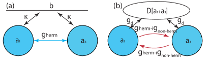
Figure 5: (a) The scheme of trion (three connected micropillar) with a rapidly decaying polariton ”b”, we transformation this trion to to the non-hermitian dimer (b) with dissipative coupling [38].

VII.2 Invariant phase $\Phi$

The Hamiltonian of the cyclic triangle circuit with (see fig. 5c) with the natural frequency of harmonic oscillators $\omega_{i}$ modulated (example, acoustic modulated) at frequency $\omega_{i}$.

$$\begin{array}[]{l}{H=\sum_{i=1}^{3}{\left(\omega_{i}+A_{i}\cos\left(w_{i}t+\varphi_{i}\right)\right){\widehat{a}}_{i}^{{\dagger}}{\widehat{a}}_{i}}+}\\ {+\sum_{i\neq j}^{3}{g_{ij}{\widehat{a}}_{i}^{{\dagger}}{\widehat{a}}_{j}+h.c.}+\sum_{i=1}^{3}{\frac{U}{2}{\widehat{a}}_{i}^{{\dagger}}{\widehat{a}}_{i}^{{\dagger}}{\widehat{a}}_{i}{\widehat{a}}_{i}}}\end{array}$$ (23)

Let’s transform Hamiltonian (23) using the unitary matrix

$$U(t)=\exp\left\{\sum_{i=1}^{N}{\left(\omega_{i}t+A_{i}\sin\left(w_{i}t+\varphi_{i}\right)\right){\widehat{a}}_{i}^{{\dagger}}{\widehat{a}}_{i}}\right\}$$ (24)

Then using the transformation

$$H^{{}^{\prime}}=UHU^{{\dagger}}+i\frac{dU}{dt}U^{{\dagger}}$$ (25)

We get the following Hamiltonian

$$H^{{}^{\prime}}=\sum_{i\neq j}^{N}{g_{ij}e^{i{\overline{\mathrm{\Delta}}}_{ij}(t)}{\widehat{a}}_{i}^{{\dagger}}{\widehat{a}}_{j}+h.c.}+\sum_{i=1}^{N}{\frac{U}{2}{\widehat{a}}_{i}^{{\dagger}}{\widehat{a}}_{i}^{{\dagger}}{\widehat{a}}_{i}{\widehat{a}}_{i}}$$ (26)

where ${\overline{\mathrm{\Delta}}}_{ij}(t)=\left(\omega_{i}-\omega_{j}\right)t+A_{i}\sin\left(w_{i}t+\varphi_{i}\right)-A_{j}\sin\left(w_{j}t+\varphi_{j}\right)=\mathrm{\Delta}_{ij}t+A\sin\left({\mathrm{\Delta}w}_{ij}t+{\mathrm{\Delta}\varphi}_{ij}\right)$; here $\mathrm{\Delta}_{ij}=\left(\omega_{i}-\omega_{j}\right),{\mathrm{\Delta}w}_{ij}=\frac{\left(w_{i}-w_{j}\right)}{2},{\mathrm{\Delta}\varphi}_{ij}=\frac{\left(\varphi_{i}-\varphi_{j}\right)}{2},$ and $\cos\left(\frac{\left(w_{i}+w_{j}\right)}{2}t+\frac{\left(\varphi_{i}+\varphi_{j}\right)}{2}\right)\approx\frac{1}{2}$; we consider it a slow variable, we also assumed that $A_{i}=A_{j}=A$.

The nonlinear part of the Hamiltonian (23) does not change in (26), since it commutes with the unitary operator (26), we can expand the exponential in a series in Bessel functions

$$e^{i{\overline{\mathrm{\Delta}}}_{ij}(t)}=e^{i\mathrm{\Delta}_{ij}t}\sum_{n=-\infty}^{\infty}{J_{n}(-A)e^{-in{\mathrm{\Delta}w}_{ij}t}e^{-in{\mathrm{\Delta}\varphi}_{ij}}}.$$ (27)

Take only the first term in the expression 27 and ${\mathrm{\Delta}w}_{ij}=$ $\mathrm{\Delta}_{ij}$, then the linear part of Hamiltonian 23 takes the form

$${H^{{}^{\prime}}}_{l}=\sum_{i\neq j}^{3}{{g^{{}^{\prime}}}_{ij}e^{-i{\mathrm{\Delta}\varphi}_{ij}}{\widehat{a}}_{i}^{{\dagger}}{\widehat{a}}_{j}+h.c.}$$ (28)

It can be easily shown that such a Hamiltonian is invariant to the gauge transformation $a\rightarrow ae^{i\phi}$ only if it is not closed in a cycle.

VII.3 Schrodinger equation for trion

Following [11] and neglecting quantum jumps, we can write the equation governing for the time dependency n-particles state $|\psi^{(n)}(t)\rangle$ for the non-Hermitian Hamiltonian:

$$i\frac{d}{dt}|\psi^{(n)}(t)\rangle\approx H_{0}|\psi^{(n)}(t)\rangle+H_{+}|\psi^{(n-1)}(t)\rangle,$$ (29)

Here we introduce the Hamiltonian that does not change the number of particles $H_{0}=\hat{a}^{+}\mathbf{G_{eff}}\hat{a}+\sum_{i}{U_{i}\hat{a}^{+}_{i}\hat{a}^{+}_{i}\hat{a}_{i}\hat{a}_{i}}$ and increases the number of particles by one $H_{+}=\sum_{i}{F_{i}\hat{a}_{i}^{+}}$ and neglecting the annihilation part of the pump Hamiltonian for weak pump limit due to sub-leading ordered $c^{(n+1)}\ll c^{(n)}$ [11].

We can obtained the recursive system equations for the $n$-state amplitude vector $c^{(n)}=(c_{n,0,0},c_{n-1,1,0},c_{n-1,0,1},...,c_{n-i,i,0},c_{n-i,i-1,1},...,c_{n-i,i-j,j},\\ ...,c_{n-i,0,i},...,c_{0,0,n})^{T}$ (which are contain $T_{n+1}$ elements, where $T_{n}=\frac{(1+n)n}{2}$ triangular numbers) by projection of Schrödinger equation (29) on bra-vector $\langle\psi^{(n)}(t)|$,

$$c^{(n)}=(-1)^{n}\prod\limits_{i=n}^{1}G^{{(i)}^{-1}}f^{(i)}$$ (30)

Where we introduce the matrix $f^{(n)}$ size $T_{n}$ by $T_{n+1}$ and the follow matrix elements

$$\begin{array}[]{l}{f^{(n)}_{s,s^{\prime}}=F_{1}\sqrt{n-m_{1}}\delta_{s_{1},s^{\prime}}+F_{2}\sqrt{m_{1}-m_{2}}\delta_{s_{2},s^{\prime}}+}\\ {+F_{3}\sqrt{m_{2}}\delta_{s_{3},s^{\prime}}}\end{array}$$ (31)

And the matrix $G^{(n)}$ size $T_{n+1}$ by $T_{n+1}$ with the follow matrix elements

$$\begin{array}[]{l}{G^{(n)}_{s,s^{\prime}}=\sum_{i=1,2,3}{(\tilde{\Delta_{i}}n_{i}+U_{i}n_{i}(n_{i}-1))\delta_{s,s^{\prime}}}}\\ {+g_{i,j}\sqrt{n_{i}(n_{j}-1)}\delta_{s_{ij},s^{\prime}}},\end{array}$$ (32)

where

$$\begin{array}[]{l}{s_{12}=1+k+\frac{1}{2}(1-n_{1}+n)(2-n_{1}+n),}\\ {s_{21}=1+k+\frac{1}{2}(n_{1}-n)(1+n_{1}-n),}\\ {s_{23}=2+k+\frac{1}{2}(n-n_{1})(1-n_{1}+n),}\\ {s_{32}=k+\frac{1}{2}(n-n_{1})(1-n_{1}+n),}\\ {s_{31}=k+\frac{1}{2}(n_{1}-n)(1+n_{1}-n),}\\ {s_{13}=2+k+\frac{1}{2}(1-n_{1}+n)(2-n_{1}+n),}\\ {s_{1}=1+k+\frac{1}{2}(n-n_{1})(1-n_{1}+n),}\\ {s_{2}=1+k+\frac{1}{2}(n-1-n_{1})(n-n_{1}),}\\ {s_{3}=k+\frac{1}{2}(n-1-n_{1})(n-n_{1}),}\\ {n_{1}=n-m_{1},}\\ {n_{2}=m_{1}-m_{2},}\\ {n_{3}=m_{2}.}\end{array}$$ (33)

here $m_{1}=[\frac{1}{2}(-1+\sqrt{8s-7})],m_{2}=[\frac{1}{2}(-1+\sqrt{8s-7-4m_{1}(m_{1}+1)})]$, where $[.]$ stands for the integer part of number in notation of Iverson.

Example,

$$f^{(2)}=\begin{bmatrix}\sqrt{2}F_{1}&0&0\\ F_{2}&F_{1}&0\\ F_{3}&0&F_{1}\\ 0&\sqrt{2}F_{2}&0\\ 0&F_{3}&F_{2}\\ 0&0&\sqrt{2}F_{3}\end{bmatrix},$$ (34)

$$G^{(2)}=\begin{bmatrix}2U+2\Delta_{1}&\sqrt{2}g_{12}&\sqrt{2}g_{13}&0&0&0\\ \sqrt{2}g_{21}&\Delta_{1}+\Delta_{2}&g_{23}&\sqrt{2}g_{12}&g_{13}&0\\ \sqrt{2}g_{31}&g_{32}&\Delta_{1}+\Delta_{3}&0&g_{12}&\sqrt{2}g_{13}\\ 0&\sqrt{2}g_{21}&0&2U+2\Delta_{2}&\sqrt{2}g_{23}&0\\ 0&g_{31}&g_{21}&\sqrt{2}g_{32}&\Delta_{2}+\Delta_{3}&0\\ 0&0&\sqrt{2}g_{31}&0&\sqrt{2}g_{32}&2U+2\Delta_{3}\end{bmatrix}$$ (35)

VII.4 Number of invariant phases on the graph

Imagine the Hamiltonian cycle

$$H=\sum_{|j-i|=1}^{N}g_{ij}e^{-i\phi_{ij}}\hat{a}_{i}^{\dagger}\hat{a}_{j}+h.c.$$ (36)

where $\phi_{ij}$ - is a phase coupling.

The invariant gauge $a_{i}\rightarrow a_{i}e^{is_{i}}$ cannot eliminate the phase coupling if the determinant of the graph’s adjacency matrix is zero. The determinant of the adjacency matrix of a closed graph is zero.

By calibration, all phases can be grouped into one phase $\Phi=\sum_{|j-i|=1}^{N}\phi_{ij}$ via the follow procedure:

$$s_{1}=-\phi_{N},s_{2}=s_{1}-\phi_{1},s_{3}=s_{2}-\phi_{2},...s_{N-1}=s_{N-2}-\phi_{N-2},s_{N}=0.$$ (37)

where $\phi_{ii-1}\equiv\phi_{i}$ is independent phase.

Let’s connect two arbitrary non-adjacent nodes $1$ and $j$ in a cyclic graph - we get two cyclic graphs. The sum of the phases on each of them may differ, for first subset 1,…,j with $\Phi_{1}=\sum_{i=1}^{j-1}\phi_{i}+\phi_{N+1}$ and second subset j+1,…,N with $\Phi_{2}=\sum_{i=j-1}^{N}\phi_{i}+\phi_{N+1}$. It can be shown that it is possible to calibrate the phases to different edges for each graph, but it is impossible to calibrate to a common edge. Let’s carry out the $\eqref{Eq19_}$ procedure for the first graph and obtain for common vertices (for the second graph): $s_{1}=-\phi_{N+1},s_{j}=0$. The same result will be obtained if we apply $\eqref{C9_}$ to the second graph, see fig. 2a. Therefore, the $\eqref{C9_}$ procedure works for calibrations of this type and no contradictions arise.

If we assume a phase on a common edge, see fig. 2b, we get the follow systems equations:

$$\begin{array}[]{l}{s_{2}-s_{1}+\phi_{1}=0}\\ {s_{3}-s_{2}+\phi_{2}=0}\\ {...}\\ {s_{j}-s_{j-1}+\phi_{j}=0}\\ {s_{1}-s_{j}+\phi_{N+1}=\Phi}\end{array}$$ (38)

and

$$\begin{array}[]{l}{s_{N}-s_{1}+\phi_{N}=0}\\ {s_{N-1}-s_{N}+\phi_{N-1}=0}\\ {...}\\ {s_{j}-s_{j+1}+\phi_{j+1}=0}\\ {s_{1}-s_{j}+\phi_{N+1}=\Phi},\end{array}$$ (39)

adding equations in each the systems $\eqref{C10_}$ and $\eqref{C11_}$ and equating them, obtain:

$$\sum_{i=1}^{j-1}\phi_{i}=\sum_{i=j-1}^{N}\phi_{i},$$ (40)

which contradicts the independence of the phases.

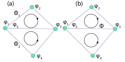
Figure 6: graph scheme (a) different invariant phases and (b) common phase.

References

- [1] T. Chanda, L. Barbiero, M. Lewenstein, M. J. Mark, and J. Zakrzewski, arXiv:2405.07775 (2024).
- [2] R. B. Wu, B. Chu, D. H. Owens, and H. Rabitz, Phys. Rev. A 97, 042122 (2018).
- [3] T. C. H. Liew and V. Savona, Phys. Rev. Lett. 104, 183601 (2010).
- [4] Chakram, S. et al. Phys. Rev. Lett. 127, 107701 (2021).
- [5] S. Ghosh and T. C. H. Liew, npj Quantum Information 6 (2020), 10.1038/s41534-020-0244-x.
- [6] F. Arute, K. Arya, R. Babbush, D. Bacon, J. C. Bardin, R. Barends, R. Biswas, S. Boixo, F. G. Brandao, D. A. Buell,et al., Nature 574.7779 (2019): 505-510.
- [7] A. Blais, S. M. Girvin, and W. D. Oliver, Nature Physics 16, 247 (2020).
- [8] K.O. Greulich and E. Thiel, Single Mol. 2, 5 (2001).
- [9] H. Wang, Y. M. He, T. H. Chung, H. Hu, Y. Yu, S. Chen, X. Ding, M. C. Chen, J. Qin, X. Yang, et al., Nature Photonics 13, 770 (2019).
- [10] A. J. Bennett, D. C. Unitt, P. Atkinson, D. A. Ritchie, and A. J. Shields, Opt. Express 13, 50 (2005).
- [11] Y. Wang, W. Verstraelen, B. Zhang, T. C. H. Liew, and Y. D. Chong, Phys. Rev. Lett. 127, 240402 (2021).
- [12] D. N. Klyshko, Usp. Fiz. Nauk 166, 613 (1996)
- [13] D. Sanvitto, F. Laussy, and D. Gerace, Nature Mater. 18, 200 (2019).
- [14] A. Miranowicz, M. Paprzycka, Y. X. Liu, J. Bajer, and F. Nori, Phys. Rev. A 87, 023809 (2013).
- [15] Rabl P. Phys. Rev. Lett. 107, 063601 (2011)
- [16] E. Zubizarreta Casalengua, J. C. López Carreño, F. P Laussy, and E. del Valle, Laser Photon. Rev. 1900279 (2020), 10.1002/lpor.201900279.
- [17] Flayac, H. and Savona, V. Unconventional Photon Blockade. Phys. Rev. A 96, 053810 (2017).
- [18] H. Paul, “Photon antibunching,” Rev. Mod. Phys. 54, 1061–1102 (1982).
- [19] H. Z. Shen, Y. H. Zhou, and X. X. Yi., Phys. Rev. A 90, 023849 (2014).
- [20] H. J. Snijders, J. A. Frey, J. Norman, H. Flayac, V. Savona, A. C. Gossard, J. E. Bowers, M. P. van Exter, D. Bouwmeester, and W. Löffler, Phys. Rev. Lett. 121, 043601 (2018).
- [21] Flayac, H. and Savona, V. Phys. Rev. A 96, 053810 (2017).
- [22] ] C. Schneider, M. M. Glazov, T. Korn, S. Höfling, and B. Urbaszek, Nat. Communs. 9, 2695 (2018).
- [23] F. P. Laussy, E. del Valle, and C. Tejedor, Phys. Rev. Lett. 101, 083601 (2008).
- [24] G. Börk, S. Machida, Y. Yamamoto, and K. Igeta, Phys. Rev. A 44, 669 (1991).
- [25] U. Oesterle, R. P. Stanley, R. Houdr´e, M. Gailhanou, and M. Ilegems, J. Cryst. Growth, vol. 150, pp. 1313–1317, (1995).
- [26] A. S. Brichkin, S. I. Novikov, A. V. Larionov, V. D. Kulakovskii, M. M. Glazov, C. Schneider, S. Höfling, M. Kamp, and A. Forchel, Phys. Rev. B 84, 195301 (2011).
- [27] Lukoshkin, V. A., V. K. Kalevich, M. M. Afanasiev, K. V. Kavokin, Z. Hatzopoulos, P. G. Savvidis, E. S. Sedov, and A. V. Kavokin, Phys. Rev. B 97, 195149 (2018).
- [28] B. Zhang, Z. Wang, S. Brodbeck, C. Schneider, M. Kamp, S. Höfling, and H. Deng, Light Sci. Appl. 3, e135 (2014).
- [29] S. Reitzenstein and A. Forchel, Journal of Physics D-Applied Physics 43, 033001 (2010).
- [30] M. Galbiati, L. Ferrier, D. D. Solnyshkov, D. Tanese, E. Wertz, A. Amo, M. Abbarchi, P. Senellart, I. Sagnes, A. Lemaître, E. Galopin, G. Malpuech, and J. Bloch, Phys. Rev. Lett. 108, 126403 (2012).
- [31] O. Gazzano, S. M. de Vasconcellos, C. Arnold, A. Nowak, E. Galopin, I. Sagnes, L. Lanco, A. Lemaître, and P. Senellart, Nat. Commun. 4, 1425 (2013).
- [32] N. Somaschi, V. Giesz, L. De Santis, J. C. Loredo, M. P. Almeida, G. Hornecker, S. L. Portalupi, T. Grange, C. Anton, J. Demory, C. Gomez, I. Sagnes, N. D. Lanzillotti Kimura, A. Lemaitre, A. Auffeves, A. G. White, L. Lanco, P. Senellart, Nat. Photonics 10, 340 (2016).
- [33] A. Verger, C. Ciuti, I. Carusotto, Phys Rev. B, 73, 193306 (2006).
- [34] H. Eleuch, J. Phys. B 41, 055502 (2008).
- [35] T. A. Khudaiberganov, I. Yu. Chestnov, and S. M. Arakelian, Appl. Phys. B 128, 117 (2022).
- [36] S. Klembt, T. H. Harder, O. A. Egorov, K. Winkler, R. Ge, M. A. Bandres, M. Emmerling, L. Worschech, T. C. H. Liew, M. Segev, C. Schneider, and S. Höfling, Nature (London) 562, 552 (2018).
- [37] A.V. Nalitov, D.D. Solnyshkov, and G. Malpuech Phys. Rev. Lett. 114, 116401 (2015).
- [38] A. A. Clerk, SciPost Phys. Lect. Notes, 44 (2022). 10.21468/SciPostPhysLectNotes.44
- [39] S. Michaelis de Vasconcellos et al., Appl. Phys. Lett. 99, 101103 (2011).
- [40] M. M. Glazov, H. Ouerdane, L. Pilozzi, G. Malpuech, A. V. Kavokin, and A. D’Andrea, Phys. Rev. B 80, 155306 (2009).
- [41] B. Villa, A. J. Bennett, D. J. P. Ellis, J. P. Lee, J. SkibaSzymanska, T. A. Mitchell, J. P. Griffiths, I. Farrer, D. A. Ritchie, C. J. B. Ford, and A. J. Shields, Appl. Phys. Lett. 111, 011103 (2017).
- [42] Holevo, A. S. ”Statistical structure of quantum theory.” Springer Science and Business Media (2001).
- [43] J. Johansson, P. Nation, and F. Nori, Comput. Phys. Commun. 184, 1234 (2013).
- [44] M. Vladimirova, S. Cronenberger, D. Scalbert, K. V. Kavokin, A. Miard, A. Lemaître, J. Bloch, D. Solnyshkov, G. Malpuech, and A. V. Kavokin, Phys. Rev. B 82, 075301 (2010).
- [45] R. Huang, A. Miranowicz, J. Q. Liao, F. Nori, and H. Jing, Nonreciprocal Photon Blockade, Phys. Rev. Lett. 121, 153601 (2018).
- [46] A. Dousse, J. Suffczynski, A. Beveratos, O. Krebs, A. Lemaître, I. Sagnes, J. Bloch, P. Voisin, and P. Senellart, Nature 466, 217 (2010).
- [47] A. Miranowicz, M. Bartkowiak, X. Wang, Y. X. Liu, and F. Nori, Phys. Rev. A 82, 013824 (2010).
- [48] M. Hillery and M. S. Zubairy, Phys. Rev. Lett. 96, 050503 (2006).