The Most Sensitive Radio Recombination Line Measurements Ever Made of the Galactic Warm Ionized Medium
Abstract
Diffuse ionized gas pervades the disk of the Milky Way. We detect extremely faint emission from this Galactic Warm Ionized Medium (WIM) using the Green Bank Telescope to make radio recombination line (RRL) observations toward two Milky Way sight lines: G20, =, and G45, =. We stack 18 consecutive Hn transitions between 4.3–7.1 GHz to derive spectra that are sensitive to RRL emission from plasmas with emission measures EM 10 . Each sight line has two Gaussian shaped spectral components with emission measures that range between 100 and 300 . Because there is no detectable RRL emission at negative LSR velocities the emitting plasma must be located interior to the Solar orbit. The G20 and G45 emission measures imply RMS densities of 0.15 and 0.18, respectively, if these sight lines are filled with homogeneous plasma. The observed / line ratios are consistent with LTE excitation for the strongest components. The high velocity component of G20 has a narrow line width, 13.5, that sets an upper limit of 4,000 K for the plasma electron temperature. This is inconsistent with the ansatz of a canonically pervasive, low density, 10,000 K WIM plasma.
1 The Milky Way Warm Ionized Medium
Hoyle & Ellis (1963) were the first to suggest the existence of a layer of ionized gas along the Galactic plane with an electron density of and an electron temperature of . This was based on their Hobart, Tasmania discovery of free-free absorption at frequencies less than 10 against the synchrotron background observed at very low radio frequencies (Ellis et al., 1962; Reber & Ellis, 1956). They estimated that the ionizing radiation necessary to produce the observed free-free absorption was consistent with flux from OB stars. The dispersion of radio waves from pulsars (Tanenbaum et al., 1968) and the observation of optical emission lines (Reynolds et al., 1973) from the interstellar medium (ISM) confirmed the existence of a warm ionized medium (WIM) in the Milky Way. Detection of H emission from the diffuse ionized gas (DIG) in the edge-on spiral galaxy NGC 891 showed that other galaxies had similar warm plasmas (Dettmar, 1990; Rand et al., 1990). Here, we follow the convention of using the term “WIM” to refer to the warm ionized medium in the Milky Way and “DIG” to refer to the diffuse ionized gas in external galaxies (Haffner et al., 2009).
The WIM has been extensively studied with optical emission lines. H maps of the Galaxy show emission from almost every direction (e.g., Dennison et al., 1998; Gaustad et al., 2001; Haffner et al., 2003) with a volume filling factor larger than 0.2 (Reynolds, 1991a). Sensitive observations of two emission lines from nitrogen indicate that the WIM is about 2,000 warmer than H ii regions (Reynolds et al., 2001). Models of escaping radiation from H ii regions indicate a harder spectrum for photons capable of ionizing hydrogen but a suppression of He-ionizing photons (Wood & Mathis, 2004), consistent with observations of helium in the WIM (e.g., Reynolds & Tufte, 1995).
Although known for 60 years now, a detailed understanding of the WIM’s origin, distribution, and physical properties remains to be crafted. Because of attenuation by dust, studies of the WIM using H are mostly limited to regions near to the Sun or at high Galactic latitudes. Moreover, the relatively low spatial and spectral resolution of most H surveys cannot separate emission from the WIM with that from discrete, OB-star excited H ii regions. This is particularly a problem in the inner Galactic disk.
Two recent radio recombination line (RRL) surveys overcome these limitations. The Green Bank Telescope (GBT) Diffuse Ionized Gas Survey (GDIGS; Anderson et al., 2021) is a 4-8 RRL survey of the Milky Way disk that probes the distribution and properties of the WIM in the inner Galaxy (). GDIGS has a angular resolution of and a spectral resolution of 0.5. A complimentary survey was completed with the Five-hundred-meter Aperture Spherical radio Telescope (FAST) using RRL transitions spanning frequencies between 1–1.5 for the Galactic zone (Hou et al., 2022). FAST has an angular resolution of 3′ and a spectral resolution of 2.2. Both surveys employ line-stacking of multiple RRL transitions observed simultaneously to increase the signal to noise ratio.
Using GDIGS data, Luisi et al. (2020) created a WIM-only RRL map of the W43 star formation complex that is devoid of emission from H ii regions. Employing an empirical model that only accounts for the H ii region locations, angular sizes, and RRL intensities, they were able to reproduce the observed WIM emission (also see Belfiore et al., 2022). This supports the notion that UV photons leaking from the H ii regions surrounding O and B-type stars are the primary source of the ionization of the WIM.
The main limitation of these new RRL surveys is sensitivity. For example, GDIGS is sensitive to emission measures, EM , whereas most H surveys are several orders of magnitude more sensitive. GDIGS detects RRL emission from most directions but not at all possible velocities where H i gas exists. This may just be a sensitivity issue. For example, the GDIGS spectrum toward G20 shows no RRL emission (see discussion below).
Here, we use the GBT to search for faint RRL emission from two first Galactic quadrant sight lines: G20 and G45. These directions, at = , and = respectively, were chosen because they contain no detected discrete H ii regions, show extremely weak radio continuum emission, and have infrared emission morphologies that do not indicate any incipient star formation. Any RRL emission detected for these lines of sight would thus stem from the WIM.
2 Observations and Data Analysis
Using the GBT, we made the RRL observations during a series of sessions held between June and August of 2020 (project GBT/20A–483). Measurements were made using the C-band (4-8) receiver and the Versatile GBT Astronomical Spectrometer (VEGAS) back end. Full details of data acquisition protocols, VEGAS tuning configuration, and calibration are described in our GDIGS paper (Anderson et al., 2021). GDIGS survey data were acquired using On the Fly Mapping. Here, however, we employ total power position switching by observing an off source (Off) position for 6 minutes and then the target (On) position for 6 minutes, for a total time of 12 minutes per scan. The Off position lies well outside the Galactic plane because the WIM is expected to be distributed throughout the Galactic disk with a large volume filling factor. The Off position is offset from the On by .
We tuned VEGAS to 64 different frequencies with two orthogonal linear polarizations each. A single 12 min OffOn spectral pair thus simultaneously produces 128 independent 8192 channel spectra, each spanning a 23.4375 bandwidth. The VEGAS tuning consisted of an assortment of hydrogen RRL transitions that lie in the 4-8 bandpass of the C-band receiver. These included and transitions, where is the transition principal quantum number. For RRL transitions the frequency extremes of this tuning are H97 (7.09541 rest frequency) and H115 (4.26814 rest frequency). This large frequency range produces significant differences in the GBT beam size (the half-power beam width, HPBW) and spectral resolution. The beam size increases from 107″ for H97 to 177″ for H115 and the spectral velocity resolution decreases from 0.12 per channel for H97 to 0.20 per channel for H115.
After acquisition, the telescope data were converted into SDFITS format and then ported to the TMBIDL single dish data analysis software package (Bania et al., 2016). All subsequent data analysis reported here is done in the TMBIDL environment.
The intensity scale is determined by injecting signals from a noise diode into the signal path every other second during observations. The flux density scale is then established after data acquisition using observations of the quasar 3C 286 which is a primary flux calibrator. For the GBT at C-band frequencies this quasar is a point source whose intensity has varied by less than 1% over decades (Ott et al., 1994; Peng et al., 2000). Because the GBT gain at C-band is 2/ Jy (Ghigo et al., 2001), the 3C 286 observations allow us to determine the noise diode fluxes. Overall, this procedure establishes the intensity scale of our spectra to 5% accuracy.
To maximize our spectral sensitivity, we derive for each target sight line a single RRL spectrum for each transition, and . We do this by averaging together all the observed, usable RRL transitions for a given . We call this procedure “stacking” and the result of this averaging is a “stacked” spectrum: , , and . The RRL transitions we use to craft these stacked spectra are compiled in Appendix Table 6. Listed there for both targets are the transition, the rest frequency, and the system temperatures, , for both linear polarizations (XX and YY).
Stacking is possible because RRLs involve high- level transitions wherein adjacent levels have nearly the same energy. For example, our usable transitions span the range from H97 to H115. In LTE the expected RRL intensities would differ by a factor of 1.66 between these two transitions. The expected line profiles, and hence the spectral line widths, should, however, be similar for all these transitions. Since the primary goal here is to detect RRL emission, all usable RRL transitions can therefore be averaged together to increase the signal-to-noise ratio, producing the , , and stacked spectra.
Stacking is not a simple average of the different transitions weighted by their individual integration times and system temperatures, although of course that must be part of the procedure. Stacking must correct for several other effects: (1) each transition has a unique rest frequency and spectral velocity resolution; (2) each transition’s spectrum has a slightly different center velocity due to our VEGAS tuning; and (3) only one of the RRL transitions is Doppler tracked due to the limitations of the GBT IF system hardware. Using the procedure described below we have successfully stacked RRL spectra taken with the Arecibo telescope/“Interim Correlator” spectrometer (Roshi et al., 2005) as well as the GBT X-band receiver/ACS spectrometer (Balser, 2006).
To derive the stacked spectra reported here we: (1) inspect for each transition all the individual OffOn total power pairs and eliminate bad data; (2) calculate for each transition an average spectrum weighted by integration time and system temperature; (3) establish a common spectral velocity resolution for each transition by using a interpolation (Roshi et al., 2005) referenced to our poorest resolution, H97, spectrum; (4) align all the transitions in velocity referenced to the Doppler tracked H103 spectrum; and (5) obtain a stacked spectrum by averaging all the individual transition spectra processed in this way weighted by integration time and system temperature.
| Source | # RRLs | RMS | ||||
|---|---|---|---|---|---|---|
| (deg) | (deg) | (hrs) | (mK) | |||
| G20 | 20.0 | 0.0 | 1: | 18 | 243.1 | 0.312 |
| G20 | … | … | 2: | 22 | 302.4 | 0.288 |
| G20 | … | … | 3: | 7 | 91.0 | 0.483 |
| G45 | 45.0 | 0.0 | 1: | 18 | 207.0 | 0.343 |
| G45 | … | … | 2: | 22 | 270.8 | 0.314 |
| G45 | … | … | 3: | 7 | 79.6 | 0.518 |
The properties of the stacked spectra for the G20 and G45 sight lines are summarized in Table 1. Listed are the source name, the Galactic position, , the RRL transition order, , the number of transitions used to derive the stacked spectrum, the total integration time of the stacked spectrum, , and the root mean square (RMS) noise of the stacked spectrum after smoothing to 1 resolution. The integration times for the spectra exceed 200 hrs and the spectral RMS noise attained thereby is 300. We believe these to be the most sensitive measurements of WIM RRL emission ever made.
3 RRL Emission from WIM Plasma
3.1 The G20 and G45 Lines of Sight
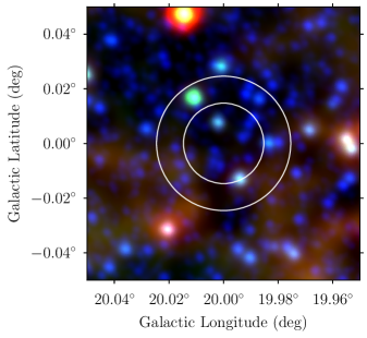
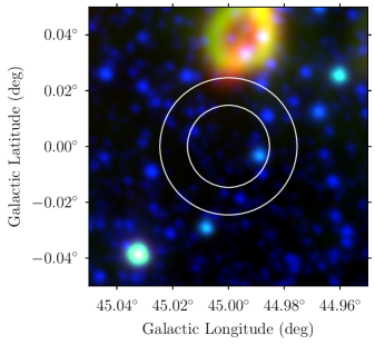
We detect weak RRL emission from both first Galactic quadrant sight lines: G20 and G45. Images of the mid-infrared emission seen toward these lines of sight by the Wide-Field Infrared Survey Explorer (Wright et al., 2010, WISE) satellite are shown in Figure 1. There is clearly no extended IR emission in these directions consistent with either protostellar activity or high mass star formation. Accordingly, the WISE Catalog of Galactic H ii Regions (Anderson et al., 2014a, hereafter “The WISE Catalog”) lists no OB-type star excited, discrete H ii regions in these fields. (The doughnut shaped object seen toward (44.99,+0.04) is a latent image from the overexposure of a saturated bright star located beyond the field of view shown in Figure 1.)
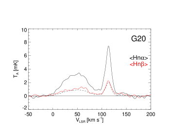
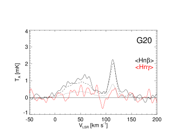
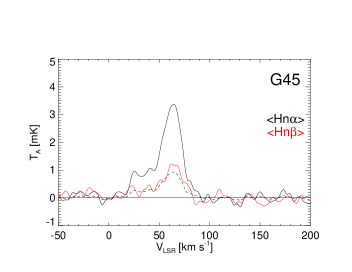
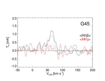
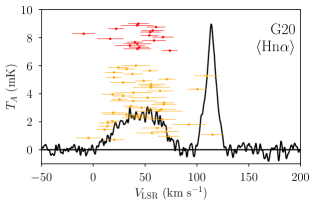
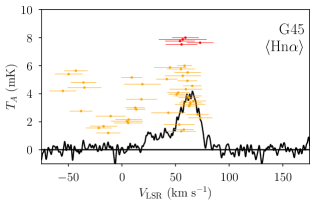
The stacked spectra we derive for G20 and G45 are shown in Figure 2. Both sight lines show two components of RRL emission from WIM plasma. In each direction the higher LSR velocity component has the stronger peak intensity and narrower line width. The G20 components are twice as strong as their corresponding G45 components. We fit Gaussian functions to these components in order to quantify their spectral line properties. Table 2 compiles the results of these fits. Listed for each spectral component are the fit values and fit errors for the LSR velocity, , peak antenna temperature at the line center, , the full width at half maximum, FWHM, line width, , the area under the component, , and an estimate of the emission measure, EM. The errors cited for peak intensity, line area, and emission measure include the 5 % uncertainty in the intensity scale.
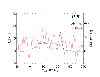
How do these spectra compare with the corresponding GDIGS and FAST measurements? Figure 3 shows that for G20 our deep integration is much more sensitive than GDIGS. GDIGS did not observe the G45 sight line but FAST did. FAST is more EM sensitive than GDIGS. Inspection of their Figure 5, however, also reveals no RRL emission. The strongest emission component that we measure toward either of our targets is therefore below the GDIGS and FAST sensitivity limits.


3.2 RRL Stacked Spectra
For both G20 and G45 RRL emission can be seen at nearly all LSR velocities between 0 and the terminal velocity produced by Galactic rotation. The lack of any detected RRL emission at LSR velocities below 0 means that in these directions any RRL emission from WIM plasma located beyond the Solar orbit about the Galactic Center must be below the sensitivity limits of our GBT observations.
| () | () | () | () | () | () | () | () | () | () | |
|---|---|---|---|---|---|---|---|---|---|---|
| G20 | 47.68 | 0.22 | 3.32 | 0.33 | 60.1 | 0.60 | 212.2 | 21.2 | 245.5 | 24.5 |
| G20 | 113.35 | 0.05 | 7.43 | 0.36 | 13.5 | 0.12 | 107.0 | 5.3 | 123.8 | 6.2 |
| G45 | 34.54 | 0.87 | 0.94 | 0.37 | 28.8 | 2.63 | 28.8 | 11.7 | 112.4 | 45.7 |
| G45 | 63.29 | 0.20 | 3.44 | 0.39 | 20.3 | 0.42 | 74.4 | 8.6 | 290.3 | 33.5 |
We use the observed RRL emission components to estimate the emission measure. Assuming that the WIM plasma is extended and always fills the GBT beam, the brightness temperature at the line center of optically thin transitions in LTE, , is [Gordon & Sorochenko (2002), Wilson et al. (2009, equation 14.28 in the 5th edition), Wenger et al. (2019, equation 16), and Anderson et al. (2021, equation A4)]:
| (1) |
where is the plasma electron temperature, is the rest frequency, and is the oscillator strength of the transition between and . We consider only transitions and adopt the average rest frequency and oscillator strength of our stacked spectra. Using these values, Equation 1 yields for the emission measure:
| (2) |
Here, [], is the spectral area of an emission component. For a Gaussian line shape, = 1.064 .
The RRL intensity values cited in all tables, however, list antenna temperature, , the directly measured quantity, rather than the brightness temperature, . Converting between antenna temperature to brightness temperature depends on the coupling between the characteristic angular size, , of the RRL emitting plasma with the GBT beam. The stacked spectra stem from frequencies spanning the 4–8 instantaneous bandwidth of the C band receiver. For this experiment, the GBT HPBW beam size, , thus ranges between 177″ for H115 to 107″ for H97. Here, we assume that the RRL emitting plasma is spatially extended and fills the GBT C band beam(s): always. For this case the brightness temperature is where the beam efficiency of the GBT at 5.7578 GHz is (Ghigo et al., 2001; Maddalena, 2010; Balser et al., 2016).
Assuming an electron temperature and FWHM line width, the observed line antenna temperature, , gives an EM of:
| (3) |
Here, we use the line peak antenna temperature, , for ease of interpreting the intensities shown in the spectra and listed in the tables. The needed conversion to brightness temperature has been absorbed into Equation 3’s numerical constant. The EM axes in Figures 2 and 3 and the values cited in Table 2 stem from Equation 3 using the observed and together with an assumed value for the plasma .
Although the electron temperature can be derived from the RRL line-to-continuum ratio, we did not measure the radio continuum for G20 and G45 and so cannot estimate from our GBT observations. Studies of the WIM/DIG in the Milky Way and other galaxies using , [N II], [S II], and [O III] find that the electron temperature ranges between 6,000 and 11,000 (Haffner et al., 2009). Here, we use the observed line widths, , to constrain . Interpreting the observed line width as being due solely to thermal broadening, = , sets a firm upper limit on the plasma electron temperature:
| (4) |
where is Boltzmann’s constant and is the mass of hydrogen. The high LSR velocity RRL components seen toward G20 and G45 have the smallest line width for each sight line. These line widths give upper limits of 4,000 and 9,000 for G20 and G45, respectively. These are the values used for the EM axes in Figures 2 and 3 and for the values cited in Table 2.
The WIM spectra we derive for G20 and G45 are very deep integrations. The four emission components that we detect toward G20 and G45 yield emission measures ranging between 100 and 300 (via Equation 2 and Table 2). All these EM values stem from smoothing the native VEGAS velocity resolution per channel to 1 . The RMS noise cited in Table 1 is for this velocity resolution. The Figure 2 spectra are thus sensitive to emission measures 20 (the 3 limit via Equation 3). Below, when we consider LTE excitation or compare RRL models to our spectra, we smooth the per channel velocity resolution to 5. At this resolution these spectra have a 3 sensitivity EM 10. Nonetheless, even then the spectra show no hint of additional emission components toward G20 and G45, especially at negative LSR velocities.
3.3 Properties of the Stacked Spectra
Before conducting further analyses of these stacked spectra, we explore how the RRL emission component line parameters vary as a function of frequency. After all, the stacked spectra are averages of many RRL transitions spanning a significant range of rest frequencies. To do this, we create “triad” spectra by stacking three consecutive Hn RRL transitions together and smoothing the resulting spectrum to 5 velocity resolution. Because our stacked spectra are comprised of 18 Hn RRL transitions, there are six of these triad spectra for each sight line and they have rest frequencies spanning the entire bandwidth of the C-band receiver. These triad spectra have the sensitivity to enable Gaussian fits for three of the four RRL emission components present in our sight lines. Only the weaker, lower velocity component of G45 cannot be analyzed this way.
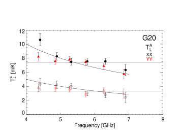
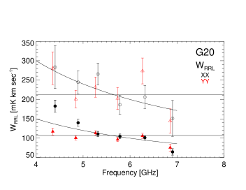
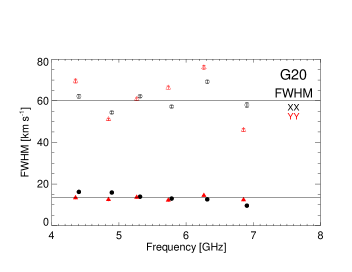
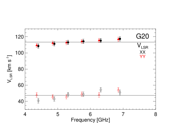
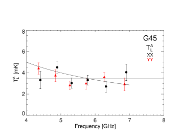
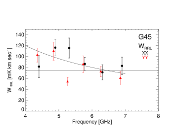
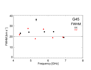
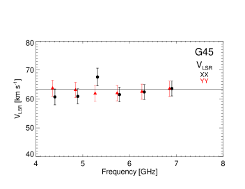
This exploration is summarized in Figure 4 for G20 and Figure 5 for G45. These figures show how the RRL emission component line parameters vary as a function of frequency. Filled symbols denote the high velocity, stronger component; open symbols show the low velocity, weaker component. For clarity, in these plots the frequency of these components has been dithered by 30. Horizontal lines flag the component parameters derived from Gaussian fits to the spectrum (Table 2).
The triad analysis shown in these figures does not reveal any issues that might compromise the stacking process. Overall, the triad data are consistent with the Table 2 Gaussian fits to the stacked spectra. Furthermore, none of the RRL emission component FWHM line widths show any systematic change with frequency. The strongest G20 emission component does have a significant LSR velocity gradient as a function of frequency. This is probably due to the changing GBT beam size sampling different volumes of plasma. Neither the weaker G20 component nor the G45 sight line component show any LSR velocity gradient.
For both sight lines, however, the triad component and values exhibit significant trends with frequency. The curves shown for and are not fits to the data, rather they are notional curves that show the frequency dependence expected for plasma in LTE and a source that fills the telescope beam (see Equation 1).
3.4 Are the G20 and G45 Plasmas in LTE?
Are the , , and stacked spectra consistent with LTE excitation? Here, we summarize our analysis of this question. The quantum mechanical details are provided in Appendix B where it shown that for our stacked spectra the expected LTE and line intensity ratios should be 0.27565 and 0.10672, respectively (see Table 8). We assess whether LTE excitation holds for our targets in two ways: (1) we scale the spectrum by the Table 8 expected LTE ratios for and RRLs and compare this in Figure 6 to our stacked and spectra; and (2) we fit Gaussian functions to the RRL emission components found in the , , and spectra and compare these in Table 3 with the expected LTE ratios. In both cases all the stacked spectra are smoothed to a velocity resolution of 5 to improve spectral sensitivity.
The first assessment of LTE is shown in Figure 6 where the left hand plots compare the and spectra for G20 and G45 with the expected LTE spectrum. The right hand plots compare the and spectra with the expected LTE intensities. Both sight lines show RRL emission that is slightly stronger than what is predicted by LTE. Although the G45 35 component matches the LTE prediction, this component is only a 1 signal. Compared with the other transitions the spectra are not very sensitive (see Table 3). Only the 50 emission component for G20 has any hint of emission and this is only a signal. For all other components we can only provide upper limits for the LTE ratio.
The second evaluation of LTE uses Gaussian fits to the individual emission components found in the stacked , , and spectra. To make the LTE assessment that is summarized in Table 3, we use the observed integrated intensity of each component, . (The slight differences in the reported fits for components that are seen when comparing Tables 2 and 3 stem from the different velocity resolutions of the spectra.)
The “LTE?” column in Table 3 gives the ratio between the observed RRL transition ratios and the expected LTE ratio. In LTE the value of this ratio of ratios would be unity. For the strongest WIM components — 113.4 for G20 and 63.3 for G45 — this ratio is and , respectively. We thus find that, within the errors, our / ratios are consistent with LTE excitation for both these emission components. The lower velocity components in these directions, however, have / ratios that are significantly larger than unity and thus are not consistent with LTE. Moreover, all ratios involving the spectra are compromised by the much poorer sensitivity of these spectra (see Appendix B).
| Source | n | LTE?aa Ratio between observed and LTE ratio (Table 8); a plasma in LTE has value unity here. | |||||||||||
|---|---|---|---|---|---|---|---|---|---|---|---|---|---|
| () | () | () | () | () | |||||||||
| G20 | 1: | 47.8 | 0.10 | 3.33 | 0.17 | 59.4 | 2.97 | 210.4 | 14.9 | 1.00 | … | … | … |
| 2: | 48.5 | 0.21 | 1.17 | 0.06 | 62.4 | 3.12 | 77.8 | 5.5 | 0.37 | 0.04 | 1.34 | 0.13 | |
| 3: | 55.3 | 0.74 | 0.74 | 0.37 | 42.0 | 2.10 | 33.1 | 16.6 | 0.16 | 0.08 | 1.48 | 0.75 | |
| G20 | 1: | 113.4 | 0.02 | 6.90 | 0.35 | 14.8 | 0.74 | 108.8 | 2.4 | 1.00 | … | … | … |
| 2: | 113.7 | 0.06 | 2.11 | 0.11 | 14.8 | 0.74 | 33.3 | 2.4 | 0.31 | 0.03 | 1.11 | 0.11 | |
| 3: | 115.8 | 0.33 | 0.54 | 0.03 | 11.4 | 0.57 | 6.5 | … | 0.06 | … | 0.56 | … | |
| G45 | 1: | 34.1 | 0.32 | 0.93 | 0.05 | 27.5 | 1.38 | 27.2 | 1.9 | 1.00 | … | … | … |
| 2: | 37.6 | 2.34 | 0.32 | 0.02 | 42.8 | 6.41 | 14.6 | 2.3 | 0.54 | 0.09 | 1.95 | 0.34 | |
| 3: | … | … | 0.50 | … | … | … | 14.9 | … | 0.55 | … | 5.14 | … | |
| G45 | 1: | 63.3 | 0.08 | 3.35 | 0.17 | 21.2 | 1.06 | 75.8 | 5.4 | 1.00 | … | … | … |
| 2: | 65.3 | 0.18 | 1.09 | 0.02 | 19.4 | 1.16 | 22.5 | 1.8 | 0.30 | 0.03 | 1.08 | 0.11 | |
| 3: | … | … | 0.20 | … | … | … | 4.5 | … | 0.06 | … | 0.56 | … |
3.5 WIM Ionization from Leakage Radiation?
WIM plasma halos envelope the PDRs that surround H ii regions ionized by OB-type stars. Case studies of individual H ii regions using RRL measurements, e.g. RCW 120 (Anderson et al., 2015) and NGC 7538 (Luisi et al., 2016), find that WIM halos are produced by stellar UV photons leaking through the PDRs and that the fraction of the leaking radio continuum emission escaping into the WIM is 25% and 15%, respectively. Furthermore, optical H studies also suggest that if OB stars are the source of the WIM ionization, then the ISM OB-type star excited H ii region distribution must allow at least 15–25% of the H-ionizing Lyman continuum photons emitted by the stars to travel hundreds of parsecs within the Galactic disk (Reynolds, 1991b).
Here, we assess whether the RRL emitting WIM plasma we find toward G20 and G45 is being ionized by leakage radiation from nearby, discrete H ii regions. The Galactic context of our sight lines is provided by the top panels of Figure 7 which show the locations and LSR velocities of all OB-type star excited H ii regions in the zone of the plots. Because we chose our targets to be devoid of obvious sources of ionizing radiation, as expected, neither sight line coincides in -space with any major concentration of H ii regions. This is especially the case for the 115 component of G20 and the 35 component of G45: neither is located on the sky near any significant number of Galactic H ii regions having their LSR velocities.
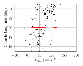
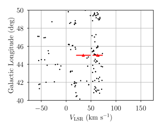
The middle panels of Figure 7 confirm that there are few Galactic H ii regions that are near both in sky location and LSR velocity to the G20 115 and G45 35 RRL emission components. These plots show the and FWHM of WISE Catalog H ii regions that are located on the sky within 100′ of the G20 and G45 sight lines plotted as a function of increasing angular separation of the nebular location from the G20 and G45 sight lines.
The nearest H ii region has the largest y-axis value. The remaining H ii regions are plotted in separation sequence with the largest separation having the smallest y-axis value. (Other than providing a co-ordinate for plotting the angular separation sequence, these y-axis values have no physical meaning.) Red points in Figure 7 are sources located within 30′ of each sight line. There are 17 and 5 WISE Catalog H ii regions located on the sky within 30′ of the G20 and G45 sight lines, respectively. Only 3 nebulae are within 10′ of our sight lines (2 for G20 and 1 for G45) and the closest H ii region lies 9′ from G45.
Some properties of these H ii regions are compiled in Appendix Table 9. Listed for each nebula is the angular separation from the fiducial line of sight (LOS), the IR radius, the Galactic position, the RRL parameters (RRL intensity, LSR velocity, and FWHM line width), together with the measurement errors. Again, the G20 115 and G45 35 components show very little correlation with known Galactic H ii regions and there are no H ii regions at these velocities within 30′ of these sight lines.
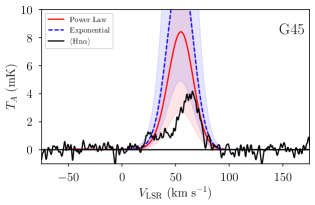
Although there are few H ii regions in close proximity to our sight lines, we may nonetheless be sensitive to extended WIM halos surrounding these nebulae. Luisi et al. (2020) develop empirical plasma halo models for the H ii region complex W43. These models reproduce the observed RRL properties of maps of the WIM surrounding W43. The models assume that the WIM RRL intensity depends only on (1) the RRL intensity of nearby H ii regions and (2) the angular distance to those H ii regions from the fiducial LOS relative to the angular size of each nebulae. For the W43 complex, they explore both an exponential and a power law WIM emission distribution model, and they find that the power law model is better able to reproduce the integrated WIM RRL intensity.
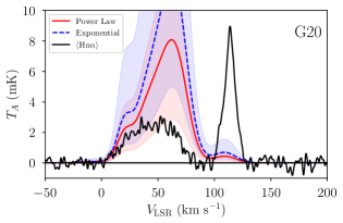
We apply the Luisi et al. (2020) models to our sight lines in order to explore the possibility that ionized halos around H ii regions can explain the WIM emission in these directions. The bottom panels of Figure 7 show the predicted RRL emission due to WIM halos around all H ii regions within 100′ of each sight line. The red solid lines show the power law model prediction,
| (5) |
and the blue dashed lines show the exponential model prediction,
| (6) |
where is the H ii region RRL spectrum, is the angular separation between the sight line and the nominal H ii region position, is the angular IR radius of the H ii region, and and are the free parameters. The H ii region RRL spectrum is evaluated from the RRL parameters in Appendix Table 9. The sum is taken over all H ii regions within 100′ of each sight line for which there is a RRL intensity measurement listed in the table. We adopt and for the power law model and and for the exponential model as determined by Luisi et al. (2020) for the W43 complex.
We note, however, two important differences between Luisi et al. (2020) and our analysis: (1) they fit their model to the integrated RRL intensity rather than the RRL spectra, and (2) they parameterize their model in terms of the average integrated RRL intensity over the H ii region rather than the “peak” RRL spectrum at the nominal H ii region position. For nebulae comparable in size to the telescope beam, the “peak” intensity is equal to the average intensity, but for angularly large nebulae the difference will depend on the emission morphology. The shaded regions in the bottom panels of Figure 7 represent the 95% confidence intervals determined by Monte Carlo resampling the H ii region RRL parameters and the model parameters and .
These empirical models, fit to the W43 complex, may not be applicable to every Galactic H ii region. By applying such models here, we inherently assume that the relative distribution of WIM emission around every H ii region is the same as that around nebulae in the W43 complex. Luisi et al. (2019) find significant variations in the radial distribution of RRL emission around several H ii regions. The magnitude of this variation is far greater than the statistical uncertainties shown in the bottom panels of Figure 7. Furthermore, the model scaling factor, , is likely related to the fraction of ionizing photons that leak into the WIM; thus probably varies from H ii region to H ii region depending on the environment.
It is thus not surprising that the bottom panels of Figure 7 show clearly that Luisi et al. (2020) models with and parameter values derived for the W43 complex do not account for the WIM RRL intensities seen toward G20 and G45. The model intensities are too high by factors of 4 and 2, respectively, for G20 and G45. These sight lines were purposely chosen not to thread through environments even remotely like those found in massive star forming regions such as W43.
Finally, it is clear from Figure 7 that the component toward G20 cannot be due to H ii region leakage radiation. No nearby H ii region is sufficiently bright or has a sufficiently narrow line width to explain this feature, as demonstrated by the Luisi et al. (2020) models and Appendix Table 9. We conclude it to be unlikely that this feature is due to extended ionized gas halos around H ii regions. It may instead constitute a heretofore unrecognized phase of the WIM (see Section 5.1). To make further progress in the exploration of the nature of plasma halos around H ii regions and this narrow RRL feature we will need sensitive RRL maps of the WIM surrounding G20 and G45. Such maps will allow us to fit Luisi et al. (2020) type models to these data.
3.6 Galactic ISM Context
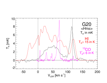
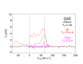
Here, we assess the Galactic context of our G20 and G45 sight lines by comparing spectra for all phases of ISM hydrogen: H+, H i, and H2. This is done in Figure 8 which shows for each sight line spectra for , 21 H i, and (10) which is a proxy for H2. These spectra were taken by different telescopes over a large range of frequencies so their beam sizes sample different LOS volumes. The WIM RRL spectra have a HPBW of . For G20 the H i spectrum is from the HI4PI all sky survey (HI4PI Collaboration et al., 2016, HPBW=). The G45 H i spectrum stems from the Boston University–Arecibo Observatory H i survey (Kuchar, 1992, HPBW=). The spectra come from the Boston University–Five College Radio Observatory Galactic Ring Survey (Jackson et al., 2006, HPBW=42″). Despite their different angular resolutions, comparing these spectra can nonetheless provide useful insights. For example, the terminal velocity, , flagged in Figure 8 is calculated for each sight line using the Clemens (1985) rotation curve. For both sight lines the H+, H i, and spectra all have emission components at or near the terminal velocity.
Our sight lines probe two important loci in the first quadrant of the Galaxy. Some key properties of these sight lines, based on an assumed Sun to Galactic Center distance, , of 8.5, are summarized in Table 4. (Other choices for would not alter the conclusions we reach here anent the spatial distribution of the WIM plasma.) Listed in Table 4 for each LOS are the minimum Galactocentric radius, = sin(), tangent point distance from the Sun, = cos(), and total path length inside the Solar orbit about the Galactic Center (GC), =2 cos().
| () | () | () | |
|---|---|---|---|
| G20 | 2.9 | 8.0 | 16.0 |
| G45 | 6.0 | 6.0 | 12.0 |
Note. — = 8.5.
Atomic hydrogen gas is ubiquitously distributed throughout the Galactic ISM. Because of this, for any line of sight 21 H i spectra show emission at all LSR velocities permitted by Galactic rotation. The velocity span of these H i spectra defines the maximum velocity spread permitted by Galactic rotation. For our first quadrant targets, gas at negative velocities is located in the Outer Galaxy beyond the Solar orbit about the Galactic Center. The Figure 8 H i spectra have emission at negative LSR velocities that extends to and for G20 and G45, respectively. In contrast, neither of our target sight lines shows any RRL emission at negative LSR velocities at the sensitivity level achieved here. G20 shows emission at all velocities between 0 and the terminal velocity whereas G45 only shows RRL emission between +20 and the terminal velocity. Assuming perfect circular rotation and no streaming motions, all of the RRL emitting gas we see toward G20 and G45 must therefore be located in the Inner Galaxy, inside the Solar orbit. This plasma must reside somewhere along the line of sight paths, , summarized in Table 4.
Unlike H i, molecular gas in the Milky Way is found in comparatively dense, discrete clouds. This means that H2/CO spectra will not have molecular emission spanning all available LSR velocities. As Figure 8 clearly shows, the molecular gas seen toward our target directions is concentrated into a few discrete emission components. At the sensitivity of the GRS, G20 shows 5 molecular clouds and G45 has but one. For both sight lines there are emission components that match the LSR velocities of the highest velocity RRL components in the spectra, albeit the 114 G20 component is extremely weak. The GRS spectrometer could not detect emission at negative LSR velocities so these spectra provide no Outer Galaxy information about molecular clouds toward these sight lines.
Cold H i embedded in a molecular cloud produces the absorption dips seen in the G20 H i spectrum at = , , and 70. These H i dips are matched by emission components. We suspect that all the components produce H i absorption but cannot definitively prove this due to a combination of mismatched angular resolution, insufficient spectral sensitivity, and the complex structure of Galactic H i spectra.
4 WIM RRL Emission Models
Here, using the emission seen from our targets, we seek to derive constraints on the line of sight density and temperature distributions of the RRL emitting plasmas. Complete details of the modeling are provided in Appendix D. Models for RRL emission from LOS plasmas must specify the electron density, , temperature, , and velocity dispersion, , at every point along the . Each model is comprised of one or more plasma “clouds” distributed along the LOS. All clouds are homogeneous, isothermal plasmas in LTE. Each cloud’s properties are specified at input. A cloud is defined by: location along the LOS, , LOS path length size (aka the cloud diameter), , electron density, electron temperature, and velocity dispersion. We use the numerical code described in Appendix D to compute synthetic spectra for H109 RRL emission from the model plasmas. After these model () RRL spectra are calculated, we compare them to spectra that are converted to brightness temperature and smoothed to 5 resolution.
We emphasize that the models are only intended to provide estimates of these quantities so we do not attempt to fully explore a large grid of parameter choices. Moreover, we do not apply any rigorous numerical metric to evaluate the “goodness of fit” between a model and the spectrum. We judge a model’s fit by eye because we can only set limits on the electron temperature.
From the observed span of these spectra we know, assuming circular rotation, that the RRL emitting plasma must be located within the Solar orbit. The simplest assumption is that a constant density isothermal plasma fills the entire in each sight line (see Table 4). For this case, the observed EM provides an estimate for the rms electron density, :
| (7) |
Table 2 shows that the total EM from the G20 and G45 emission components is 369.3 and 402.7 , respectively. This gives from Equation 7 an of 0.15 and 0.18, respectively, for these sight lines. These estimates, however, do not account for gas clumping: there may be significant gaps and/or density fluctuations in the plasma distribution along each LOS. Many different LOS distributions can produce identical values.
Due to the first Galactic quadrant distance ambiguity, we cannot know a priori where the RRL emitting plasma is located vis a vis the LOS near/far locations. A series of models seeking to find cloud parameters that produce a synthetic spectrum matching the observations confirms that there is no unique solution. A plethora of models can reproduce the spectra. Because of this, models for our target’s emission at LSR velocities having LOS distance ambiguities provide no meaningful limits for the plasma density and distribution along the LOS.
| LOS | Model | ||||||||
|---|---|---|---|---|---|---|---|---|---|
| () | () | () | () | () | () | () | () | ||
| G20 | A | 2.9 | 8.0 | 2.0 | 0.38 | 4000 | 5.7 | 289 | 1520 |
| B | 2.9 | 8.0 | 2.0 | 0.29 | 2800 | 5.7 | 168 | 812 | |
| RMS | 2.9 | 8.0 | 16.0 | 0.15 | 4000 | 5.7 | 360 | 600 | |
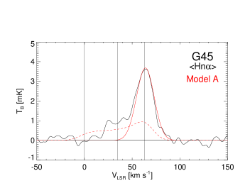
| G45 | A | 6.0 | 6.0 | 4.0 | 0.40 | 9000 | 8.6 | 640 | 3600 |
| B | 6.0 | 6.0 | 4.0 | 0.31 | 6400 | 8.6 | 384 | 1984 | |
| RMS | 6.0 | 6.0 | 12.0 | 0.18 | 9000 | 8.6 | 389 | 1620 |
4.1 LOS Tangent Point Models
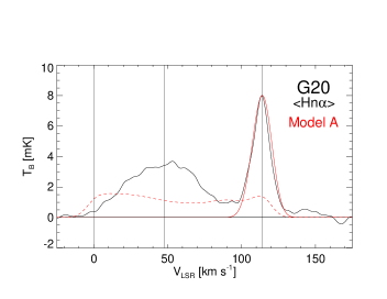
Models for RRL emitting gas located at the LOS tangent point distance, however, can provide useful constraints for the plasma physical properties. Gas is unambiguously located at the tangent point if it is emitting at the LSR terminal velocity produced by Galactic rotation for a particular first quadrant sight line. The high velocity components seen toward G20 and G45 emit at their terminal velocities and are hence located at their respective tangent point distances from the Sun.
We model the RRL emission from these components using a single cloud each for G20 and G45. Each plasma cloud is specified by its LOS distance, , cloud size, electron density, , electron temperature, , and the velocity dispersion of the emission component, . Each cloud is located at the tangent point distance (see Table 4). The velocity dispersion is set by the observed line width (see Table 2 where = /2.355 for a Gaussian line shape).
We use the observed RRL line width, , to set the model plasma electron temperature. This line width stems from a combination of mechanisms including thermal, , and non-thermal broadening, . In addition, velocity shear along the line of sight produced by Galactic rotation, , can also broaden the line emission, . (Quantum mechanical natural broadening is insignificant compared with these mechanisms.) The broadening processes add in quadrature to produce the observed line width: . By definition the line of sight LSR velocity gradient at any Galactic tangent point distance, , is . Thus, for plasma located at the tangent point, spectral broadening due to Galactic rotation, , is negligible. The WIM plasma is turbulent, however, so even at the tangent point the observed RRL line width is an unknown combination of thermal and non-thermal, supersonic turbulent broadening: .
We estimate in two ways, leading to two models each for G20 and G45. Model A sets to be the upper limit derived using Equation 4 and assuming that is entirely due to thermal broadening: =. Because the plasma is turbulent, this is a robust upper limit for . For Model A, is 4,000 and 9,000 for G20 and G45, respectively. Model B explores the effect of turbulent broadening by assuming that the thermal and turbulent contributions to the line width are equal: =. The thermal contribution to the observed line width is then =/. For Model B, is 2,800 and 6,400 for G20, and G45, respectively.
Here, we seek to reproduce both the intensity and line shape of the tangent point emission components. The model cloud parameters that are yet to be determined are the electron density and cloud size. For an isothermal plasma the RRL intensity scales linearly with emission measure so . The model spectral intensities are very sensitive to . We find that changing by 0.01 produces significant differences in the model peak intensity. The cloud size is constrained by the line shape: if the cloud is too large, Galactic rotation produces a distinctly non-Gaussian line profile.
To craft the final model parameters we explored a range of choices for and . The models are summarized in Table 5 which lists for each cloud the minimum LOS Galactocentric distance, , location along the LOS, , LOS path length size (i.e., the cloud diameter), , electron density, , electron temperature, , velocity dispersion, , emission measure, EM, and the plasma pressure, . The Model A spectra for G20 and G45 are compared in Figure 9 with the observed emission. The Model B spectra are not shown because their has been adjusted to fit the observed and so they are indistinguishable from Model A.
The dashed red curve models in Figure 9 have plasma filling the entire LOS inside the solar orbit with the rms electron density from Equation 7 (see model “RMS” in Table 5). As expected these models are poor fits to the observed spectra because the plasma is surely not homogeneous and isothermal throughout the path length. The models do, however, show the LSR velocity span produced by plasma that fills the entire . For both sight lines these models produce larger intensities for ’s between 0 and 20 than what is observed. This may indicate that the plasma density is rather low near the Sun for both directions.
5 Discussion
Here, we compare our results for G20 and G45 with other studies of the WIM. This is challenging because there is no universally accepted definition of the WIM. The plasma has been investigated using a variety of spectral observations over a range of frequencies. The WIM has been studied in the optical, far infrared (FIR), and radio. Interpreting these spectra requires many different techniques and assumptions before one derives physical properties such as density and temperature. Furthermore, because of dust extinction and differing angular resolutions, these three spectral regimes probe different volumes of the Milky Way.
Historically, the distribution and physical properties of the WIM in the Milky Way have primarily been characterized by observations of optical spectral lines. H emission studies conclude that the WIM accounts for % of the ionized gas in the ISM with a scale height of (e.g., Reynolds, 1989; Hill et al., 2008). Dispersion measures from pulsars with known distances, together with H emission measures, estimate the range of the average electron density to be 0.03-0.10 with a filling factor, 0.4-0.2 (e.g., Reynolds, 1991a; Taylor & Cordes, 1993; Berkhuijsen et al., 2006; Gaensler et al., 2008). The ratio of [N ii] 5755 and [N ii] 6583 provides a direct measure of the electron temperature and indicates the WIM is about 2,000 warmer than H ii regions (Reynolds et al., 2001). For a typical H ii region with , this corresponds to an electron temperature of .
Most of the ionized gas in the Milky Way, however, is located in the inner Galaxy which is not probed by optical emission lines because of extinction by dust. Far-infrared collisionally excited lines are less affected by dust and offer an alternative method to sample the WIM. In particular, [N ii] 122 µm and [N ii] 205 µm are excellent diagnostics of the WIM since nitrogen has an ionization potential of 14.5 eV, similar to hydrogen (13.6 eV), and will thus be associated with H ii.
Using the HIFI instrument on Herschel, Persson et al. (2014) observed [N ii] 205 µm toward four H ii regions. They detected absorption of [N ii] from foreground gas toward W31C and W49N. This absorbing gas must be located within the Solar orbit due to the velocity range of the spectral components. Assuming a N/H abundance ratio and filling factor they estimate mean electron densities of . These results, together with modeling of N+ with RADEX, are consistent with the optically derived WIM properties, albeit with somewhat higher electron densities.
Observations of RRLs offer an extinction-free probe of the WIM. Early RRL observations made with single-dish telescopes toward directions away from OB-type star excited H ii regions detected weak RRL emission (e.g., Gottesman & Gordon, 1970; Lockman, 1976; Mezger, 1978; Heiles et al., 1996; Roshi & Anantharamaiah, 2000). This emission was interpreted by Mezger (1978) as being associated with the envelopes of H ii regions and called the “extended low density” (ELD) H ii. Because of their poor angular resolution, however, all these observations suffer from confusion with the known population of H ii regions (Anderson et al., 2014b) so any quantitative interpretation of these data is problematic.
The more recent RRL surveys with the GBT and FAST, however, have sufficient angular resolution to avoid emission from H ii regions and in principle produce WIM-only images (Anderson et al., 2021). But there are several reasons why these WIM-only images may still contain ELD H ii emission and thus not be truly representative of WIM gas: (1) GDIGS is only sensitive to plasmas with mean electron densities (for a path length of 1) and this is 100 times larger than the density expected for the WIM (see the Figure 3 sensitivity comparison); (2) since H studies imply that the WIM fills 70% of the ISM’s volume, this semi-ubiquitously distributed plasma ought to emit over the entire range of velocities that are allowed by Galactic rotation yet for typical sight lines the GDIGS detected RRL spectra have gaps with no emission at allowed LSR velocities; and (3) the RRL emission appears to be correlated with the location of H ii regions (Luisi et al., 2020) and therefore may be part of the ELD H ii.
For the high sensitivity RRL observations toward G20 and G45, we estimate rms electron densities of over a wide range of velocities. For a filling factor of this corresponds to mean electron densities of . These electron densities are somewhat higher than expected from the WIM based on optical data. These higher values may not be surprising since Figure 7 suggests that some of the emission detected toward both G20 and G25 might be associated with OB-type star H ii regions. But the figure also shows that the G20 RRL emission above 100 and the G45 emission below 50 have no association with any nearby H ii regions and are probably tracing the WIM.
5.1 G20
The narrow, 13.5, line width from plasma located at the G20 tangent point distance sets a strong upper limit of 4,000 K on the electron temperature. At this , Model A with a density of =0.38 replicates the observed intensity and line shape of this emission component. The Model A pressure is 1,520 . Models A and B together span between 0.38–0.29 and between 4,000–2,800 resulting in WIM pressures ranging from 1,500 to 800 .
Measuring the pressure in the WIM is challenging because there do not seem to be any observables from which one can derive both the density and temperature without bias. Combining the pulsar/H91 density determinations with the FIR derived electron temperature yields a nominal pressure, , of 500 to 1,000 for the WIM plasma. But combining these and determinations may be problematic. For example, these estimates for the WIM plasma’s physical parameters are not probing the same gas volumes. In lieu of robust observational constraints for the WIM , we can seek insight from simulations. The TIGRESS-NCR simulation of the Galactic ISM (Kim et al., 2023) predicts a WIM pressure ranging between and , with a mean value close to .
Here, we show that a combination of RRL observations with models for the emission together provide an alternative approach to deriving the WIM pressure. Using the observed RRL line width to constrain and models to estimate , we find that the pressure derived here for the G20 tangent point emission is generally consistent with other determinations of the WIM pressure that are based on observations. The low limit, however, is not. Too, the electron density is at the high end for values typically derived for WIM plasma. Altogether, the G20 model for the tangent point emission challenges our understanding of the WIM as a canonically pervasive, low density, 0.1 , 10,000 plasma.
5.2 G45
The line width, 20.3, for the G45 tangent point emission component also sets a strong upper limit for the plasma electron temperature of 9,000 . Model A adopts this limit and with a density of =0.40 replicates the observed intensity and line shape of this emission component. Models A and B together span between 0.40–0.31 and between 9,000–6,400 resulting in WIM pressures ranging from 3,600 to 2,000 .
These model pressures are also consistent with other determinations of the WIM pressure and are more in line with the TIGRESS-NCR simulation results. Again, the density is at the high end of values reported for the WIM, but overall this G45 tangent point emission component’s physical properties are consistent with WIM plasma.
In sum, the result of these efforts is that the WIM spans a range of densities. Almost any density up to a few may be consistent with the WIM. Optical studies derive 0.03–0.1 (Haffner et al., 2009). FIR observations of fine structure transitions infer 0.1–0.3 (Persson et al., 2014). Our G20 and G45 analysis gives 0.3–0.4. Finally, there is evidence from low frequency RRL observations for a more or less continuous distribution of plasma densities. Several studies have found volume filling factors inversely proportional to density, so the higher densities subsume an increasingly smaller fraction of the ISM volume (e.g., Anantharamaiah, 1985, 1986; Roshi & Anantharamaiah, 2001).
6 Summary
Studies of the Milky Way’s WIM that use H emission can only probe the Galactic disk out to distances limited to a few from the Sun due to extinction. Because the ISM is optically thin at cm wavelengths radio recombination lines probe the WIM emission at transgalactic path lengths. Here, we use RRL emission to study two Galactic sight lines located in the plane that are devoid of any OB-star produced H ii regions and show no indication of nearby star formation.
-
•
GBT observations of the WIM made toward Galactic sight lines G20 and G45 show four Gaussian-shaped emission features in the stacked RRL spectra. The emission measures of these spectral components range between 100 and 300.
-
•
For both sight lines, RRL emission can be seen at nearly all LSR velocities between 0 and the terminal velocity produced by Galactic rotation. The lack of any significant RRL emission at LSR velocities below 0 means that in these directions RRL emission from any WIM plasma located beyond the Solar orbit is below the EM 10 (3 limit for 5 resolution) sensitivity limit of our GBT observations. For G20 and G45, the line of sight path lengths with RRL emitting WIM plasma, , must thus be no larger than 12 and 16 , respectively.
-
•
The observed / intensity ratios are consistent with LTE excitation for the stronger, higher velocity components seen toward both sight lines at LSR velocities of 113 and 63 for G20 and G45, respectively. The weaker, lower velocity components at 48 and 35 , however, show some evidence for non-LTE excitation.
-
•
Although our sight lines show no H ii regions in their fields, the WIM emission we observe might originate in extended WIM halos around H ii regions. Some of the emission detected toward both G20 and G45 occurs at LSR velocities shared with nearby H ii regions. Empirical models for WIM emission near H ii regions predict comparable emission to what is seen (see Figure 7), although the model uncertainties preclude us from making any definitive conclusions. Despite these uncertainties, it seems unlikely that the G20 RRL emission above 100 is associated with nearby known H ii regions.
-
•
Cloud models with plasma located at the G20 and G45 tangent points reproduce the observed RRL emission components at the tangent point velocities for these sight lines. These models have densities = 0.29– 0.40 , temperatures = 2,800– 9,000 , and pressures 800– 3,600 .
-
•
The pressure derived for the G20 tangent point emission is consistent with other determinations of the WIM pressure. The low, 4,000 limit, however, is not. The G20 model for the tangent point emission challenges our understanding of the WIM as a canonically pervasive, low density, 0.1 , 10,000 plasma.
Appendix A RRL Transitions used for Stacked Spectra
Instrumental effects caused by the C-band receiver, the GBT IF system, and VEGAS spectrometer compromise some of the transitions we observe. These effects include unacceptable frequency structure in the spectral baselines and loss of sensitivity due to high system temperatures. High system temperatures mostly occur when the C-band receiver performance deteriorates at both the high and low frequency extremes of the 4 bandwidth. We inspected each RRL tuning to evaluate overall quality. The usable RRL transitions are summarized in Table 6. Listed for the G20 and G45 targets are the transition, the rest frequency, and the average system temperatures for both linear polarizations: and . For these acceptable tunings system temperatures typically range between 20 and 40.
| Line | Transition | Frequency | TXX | TYY | TXX | TYY |
|---|---|---|---|---|---|---|
| (GHz) | (K) | (K) | (K) | (K) | ||
| H97 | 98 97 | 7.09541 | 38.6 | 38.3 | 38.0 | 37.4 |
| H98 | 99 98 | 6.88149 | 35.4 | 33.4 | 34.6 | 31.9 |
| H99 | 100 99 | 6.67607 | 35.8 | 27.6 | 35.1 | 26.5 |
| H100 | 101 100 | 6.47876 | 24.6 | 25.1 | 23.9 | 24.1 |
| H101 | 102 101 | 6.28914 | 29.8 | 21.1 | 28.5 | 20.2 |
| H102 | 103 102 | 6.10685 | 28.5 | 21.7 | 27.6 | 20.8 |
| H103 | 104 103 | 5.93154 | 26.9 | 22.8 | 25.8 | 21.8 |
| H104 | 105 104 | 5.76288 | 24.2 | 23.4 | 23.0 | 22.4 |
| H105 | 106 105 | 5.60055 | 23.8 | 24.0 | 22.5 | 22.8 |
| H106 | 107 106 | 5.44426 | 21.2 | 24.2 | 20.1 | 23.1 |
| H107 | 108 107 | 5.29373 | 27.1 | 23.7 | 25.6 | 22.5 |
| H108 | 109 108 | 5.14870 | 24.6 | 26.4 | 23.1 | 25.1 |
| H109 | 110 109 | 5.00892 | 25.8 | 24.1 | 24.0 | 22.8 |
| H110 | 111 110 | 4.87416 | 26.0 | 24.0 | 24.2 | 22.8 |
| H111 | 112 111 | 4.74418 | 27.0 | 23.7 | 24.9 | 22.5 |
| H112 | 113 112 | 4.61879 | 27.1 | 25.2 | 25.2 | 24.0 |
| H114 | 115 114 | 4.38095 | 30.2 | 32.4 | 27.6 | 30.7 |
| H115 | 116 115 | 4.26814 | 38.9 | 39.1 | 36.0 | 36.0 |
| H122 | 124 122 | 7.06872 | 34.1 | 35.0 | 33.3 | 34.8 |
| H123 | 125 123 | 6.89905 | 34.6 | 32.9 | 33.7 | 31.8 |
| H124 | 126 124 | 6.73479 | 34.0 | 31.3 | 33.1 | 29.9 |
| H125 | 127 125 | 6.57570 | 27.7 | 26.4 | 26.7 | 25.1 |
| H126 | 128 126 | 6.42158 | 24.5 | 29.8 | 23.7 | 28.6 |
| H127 | 129 127 | 6.27223 | 30.3 | 22.4 | 29.2 | 21.4 |
| H128 | 130 128 | 6.12748 | 31.0 | 22.2 | 29.4 | 21.2 |
| H129 | 131 129 | 5.98714 | 28.8 | 22.5 | 27.6 | 21.5 |
| H130 | 132 130 | 5.85107 | 25.5 | 22.6 | 24.3 | 21.5 |
| H131 | 133 131 | 5.71909 | 24.3 | 23.1 | 23.1 | 21.9 |
| H132 | 134 132 | 5.59105 | 24.3 | 23.9 | 23.2 | 22.8 |
| H133 | 135 133 | 5.46680 | 22.5 | 23.3 | 21.2 | 22.0 |
| H134 | 136 134 | 5.34619 | 21.7 | 25.7 | 20.5 | 24.3 |
| H135 | 137 135 | 5.22913 | 25.6 | 17.3 | 23.8 | 16.3 |
| H136 | 138 136 | 5.11544 | 26.4 | 22.9 | 24.8 | 21.8 |
| H137 | 139 137 | 5.00502 | 25.4 | 24.1 | 23.8 | 22.8 |
| H138 | 140 138 | 4.89778 | 25.9 | 24.2 | 24.0 | 23.0 |
| H139 | 141 139 | 4.79357 | 26.3 | 23.7 | 24.4 | 22.5 |
| H140 | 142 140 | 4.69229 | 28.2 | 24.8 | 25.9 | 23.3 |
| H141 | 143 141 | 4.59384 | 30.0 | 23.5 | 27.5 | 22.2 |
| H143 | 145 143 | 4.40508 | 29.9 | 30.5 | 27.4 | 28.7 |
| H145 | 147 145 | 4.22650 | 42.4 | 32.8 | 38.3 | 30.8 |
| H139 | 142 139 | 7.11476 | 40.8 | 42.4 | 39.9 | 41.4 |
| H140 | 143 140 | 6.96495 | 34.1 | 32.3 | 33.5 | 31.5 |
| H141 | 144 141 | 6.81933 | 38.5 | 32.8 | 37.5 | 31.6 |
| H143 | 146 143 | 6.54004 | 26.5 | 26.2 | 25.6 | 25.1 |
| H144 | 147 144 | 6.40609 | 23.2 | 28.7 | 22.5 | 27.6 |
| H146 | 149 146 | 6.14898 | 23.9 | 23.5 | 22.9 | 22.4 |
| H147 | 150 147 | 6.02558 | 27.6 | 23.2 | 26.4 | 22.2 |
Appendix B Radio Recombination Line Excitation Analysis
B.1 LTE Excitation
Are the , , and stacked spectra consistent with LTE excitation? To make this assessment we need to know the expected LTE ratio between a specific transition and a fiducial transition. Here, we use as the fiducial transition and calculate the LTE ratios expected for and . First we calculate the statistical weights, , and oscillator strengths, , for each RRL transition listed in Appendix Table 6. Since these transitions were used to craft the stacked spectra, we use the average statistical weight, , and average oscillator strength, , for , , and to derive the expected LTE ratios.
| Transition | ||||
|---|---|---|---|---|
| H97 | 97 | 1 | 18818 | 18.79132765 |
| H98 | 98 | 1 | 19208 | 18.98210255 |
| H99 | 99 | 1 | 19602 | 19.17287745 |
| H100 | 100 | 1 | 20000 | 19.36365235 |
| H101 | 101 | 1 | 20402 | 19.55442725 |
| H102 | 102 | 1 | 20808 | 19.74520215 |
| H103 | 103 | 1 | 21208 | 19.93597705 |
| H104 | 104 | 1 | 21632 | 20.12675195 |
| H105 | 105 | 1 | 22050 | 20.31752685 |
| H106 | 106 | 1 | 22472 | 20.50830175 |
| H107 | 107 | 1 | 22898 | 20.69907665 |
| H108 | 108 | 1 | 23328 | 20.88985155 |
| H109 | 109 | 1 | 23762 | 21.08062645 |
| H110 | 110 | 1 | 24200 | 21.27140135 |
| H111 | 111 | 1 | 24642 | 21.46217625 |
| H112 | 112 | 1 | 25088 | 21.65295115 |
| H114 | 114 | 1 | 25992 | 22.03450095 |
| H115 | 115 | 1 | 26450 | 22.22527585 |
| H122 | 122 | 2 | 29768 | 3.29151250 |
| H123 | 123 | 2 | 30258 | 3.31784460 |
| H124 | 124 | 2 | 30752 | 3.34417670 |
| H125 | 125 | 2 | 31250 | 3.37050880 |
| H126 | 126 | 2 | 31752 | 3.39684090 |
| H127 | 127 | 2 | 32258 | 3.42317300 |
| H128 | 128 | 2 | 32768 | 3.44950510 |
| H129 | 129 | 2 | 33282 | 3.47583720 |
| H130 | 130 | 2 | 33800 | 3.50216930 |
| H131 | 131 | 2 | 34322 | 3.52850140 |
| H132 | 132 | 2 | 34848 | 3.55483350 |
| H133 | 133 | 2 | 35378 | 3.58116560 |
| H134 | 134 | 2 | 35912 | 3.60749770 |
| H135 | 135 | 2 | 36450 | 3.63382980 |
| H136 | 136 | 2 | 36992 | 3.66016190 |
| H137 | 137 | 2 | 37538 | 3.68649400 |
| H138 | 138 | 2 | 38088 | 3.71282610 |
| H139 | 139 | 2 | 38642 | 3.73915820 |
| H140 | 140 | 2 | 39200 | 3.76549030 |
| H141 | 141 | 2 | 39762 | 3.79182240 |
| H143 | 143 | 2 | 40898 | 3.84448660 |
| H145 | 145 | 2 | 42050 | 3.89715080 |
| H139 | 139 | 3 | 38642 | 1.16315647 |
| H140 | 140 | 3 | 39200 | 1.17126209 |
| H141 | 141 | 3 | 39762 | 1.17936771 |
| H143 | 143 | 3 | 40898 | 1.19557895 |
| H144 | 144 | 3 | 41472 | 1.20368457 |
| H146 | 146 | 3 | 42632 | 1.21989581 |
| H147 | 147 | 3 | 43218 | 1.22800143 |
The quantum properties of the Table 6 transitions are compiled in Table 7. Listed are the transition, the principle quantum number, , the order of the transition, , the statistical weight, , and oscillator strength, . The statistical weight is and we use the prescription in Menzel (1968) to derive the oscillator strengths, , for recombination transitions between principle quantum numbers .
The LTE RRL intensity ratio between two optically thin transitions is given by the ratio of their oscillator strengths, , and their statistical weights, :
| (B1) |
Here, and refer to the fiducial transition, , and the angle brackets denote the average of the quantum properties of the transitions used to derive the stacked spectra. The average quantum properties for the , , and stacked spectra are summarized in Table 8 which lists , , and . The last column of Table 8 gives the LTE intensity ratios for and relative to .
The “LTE?” column in Table 3 gives the ratio between the observed RRL transition ratios and the expected LTE ratio. In LTE this ratio of ratios would be unity. For the strongest WIM components — 113.4 for G20 and 63.3 for G45 — this ratio is and , respectively. We thus find that, within the errors, our / ratios are consistent with LTE excitation for both sight lines.
The lower velocity components in these directions, however, give values for the “LTE?” parameter that are significantly larger than one: and for G20 and G45, respectively. Moreover, all ratios involving the spectra are compromised by the much poorer sensitivity of these spectra due to their comparatively small integration times compared with the and data. These spectra can only provide upper limits and these limits are not significant.
B.2 Non-LTE Excitation
We thus find that the lower velocity components seen in the G20 and G45 spectra show some evidence for non-LTE excitation in the WIM gas. These non-LTE effects can be described by the use of departure coefficients, . Departure coefficients relate the true level population, , to the population level under LTE, , where . Non-LTE effects can alter the RRL intensities in the following way (see Equation 14.52 in Wilson et al., 2009):
| (B2) |
where is the observed line intensity, is the LTE intensity, and is the continuum optical depth. Here, is a measure of the gradient of with respect to (see Equation 14.40 in Wilson et al., 2009):
| (B3) |
The first term in Equation B2 accounts for the effect of non-LTE line formation whereas the second describes non-LTE line transfer effects which can include maser amplification of the line radiation. When becomes negative, , maser amplification occurs and the resulting RRL intensities will depend on radiative transfer details.
For the low densities expected in the WIM, however, the continuum opacity should be small at cm-wavelengths and thus . The main non-LTE effect will therefore be departures in the level populations and so the non-LTE line intensity is the LTE intensity times : .
As the principle quantum number , approaches unity. Since increases with for RRLs at the same frequency —e.g., H102, H129, and H147 have nearly identical rest frequencies — we expect the Hn transitions to be closer to LTE than the Hn transitions. The observed intensities should thus be larger than expected when in LTE, consistent with the results in Figure 6 and Table 3.
In sum, we find that for the strongest WIM components seen in G20 and G45 the / ratios are consistent with LTE excitation. The weaker components, however, show some evidence for non-LTE excitation. The intensity can be weaker than the LTE value because collisions are less effective due the size of the H atom compared with the larger size of the nearby (in frequency) transition. For the larger atom collisions are more effective in establishing LTE level populations and the deviation from LTE is smaller. As a consequence the / ratio can exceed the LTE value.
Appendix C H II Regions Located Near the G20 and G45 Sight Lines
Properties of WISE Catalog H ii regions located within 100′ of the G20 and G45 sight lines are compiled in Table 9. Listed for each nebula are the galactic co-ordinates, , and angular separation from the sight line, together with the IR radius, , RRL intensity, , LSR velocity, , FWHM line width, , and their measurement errors. Some of the entries in the WISE Catalog refer to nebulae that reside within the same telescope beam. In those cases the Catalog lists identical and values (see Anderson et al., 2014b). When such confusion within the beam occurs we only list here (and use in Figure 7) a single nebula, choosing the one with the smallest separation from its fiducial sight line. Some WISE H ii region spectra have emission at multiple velocities. Because we have no reason to choose otherwise, in these cases we plot all the velocities in Figure 7.
| H ii Region | Separation | |||||||||
|---|---|---|---|---|---|---|---|---|---|---|
| (arcmin) | (arcmin) | (deg) | (deg) | (mK) | (mK) | () | () | () | () | |
| G020.09800.123 | 9.44 | 0.7 | 20.10 | 0.123 | 32.3 | 0.3 | 43.4 | 0.1 | 20.3 | 0.2 |
| G020.08300.135 | 9.48 | 0.5 | 20.08 | 0.134 | 31.0 | 2.8 | 42.2 | 1.4 | 31.7 | 3.3 |
| G019.818+00.010 | 10.92 | 1.9 | 19.82 | +0.010 | 26.1 | 0.4 | 60.4 | 0.1 | 18.2 | 0.3 |
| G020.227+00.110 | 15.13 | 1.2 | 20.23 | +0.110 | 10.5 | 0.2 | 22.1 | 0.2 | 14.9 | 0.4 |
| G019.72800.113 | 17.67 | 0.7 | 19.73 | 0.113 | 15.4 | 0.4 | 57.3 | 0.3 | 21.7 | 0.7 |
| G019.67700.134 | 20.96 | 1.0 | 19.68 | 0.133 | 48.0 | 5.8 | 55.0 | 1.2 | 20.0 | 2.8 |
| G019.780+00.286 | 21.65 | 1.9 | 19.78 | +0.287 | 21.3 | 0.3 | 9.3 | 0.2 | 21.7 | 0.4 |
| G020.36300.014 | 21.80 | 0.7 | 20.36 | 0.014 | 21.8 | 0.5 | 54.1 | 0.2 | 16.6 | 0.4 |
| G020.15000.335 | 22.03 | 9.4 | 20.15 | 0.335 | 19.0 | 2.9 | 67.3 | 1.5 | 20.3 | 3.6 |
| G019.741+00.280 | 22.89 | 0.7 | 19.74 | +0.280 | 32.2 | 0.4 | 16.3 | 0.1 | 25.5 | 0.3 |
| G019.62900.095 | 22.96 | 5.5 | 19.63 | 0.094 | 54.0 | 3.7 | 58.6 | 0.8 | 22.8 | 1.8 |
| G019.71600.261 | 23.11 | 1.0 | 19.72 | 0.261 | 29.6 | 0.5 | 40.1 | 0.1 | 15.2 | 0.3 |
| G019.67500.226 | 23.69 | 3.5 | 19.68 | 0.225 | 168.5 | 1.7 | 42.5 | 0.1 | 26.5 | 0.4 |
| G019.594+00.024 | 24.40 | 0.7 | 19.59 | +0.024 | 12.8 | 0.3 | 35.3 | 0.4 | 29.0 | 1.0 |
| G019.66600.309 | 27.25 | 1.2 | 19.67 | 0.308 | 33.9 | 0.8 | 44.3 | 0.2 | 19.2 | 0.5 |
| G019.60900.239 | 27.46 | 1.4 | 19.61 | 0.238 | 168.5 | 1.7 | 42.5 | 0.1 | 26.5 | 0.4 |
| G020.457+00.021 | 27.48 | 1.7 | 20.46 | +0.022 | 66.7 | 1.1 | 73.8 | 0.1 | 15.0 | 0.3 |
| G019.55400.248 | 30.60 | 3.2 | 19.55 | 0.248 | 131.0 | 7.4 | 41.0 | 0.8 | 27.7 | 1.8 |
| G020.481+00.168 | 30.63 | 2.6 | 20.48 | +0.169 | 24.0 | 2.3 | 24.1 | 1.0 | 20.5 | 2.2 |
| G019.49400.150 | 31.65 | 1.9 | 19.49 | 0.149 | 34.3 | 0.4 | 32.1 | 0.1 | 16.8 | 0.3 |
| G019.49400.150 | 31.65 | 1.9 | 19.49 | 0.149 | 20.5 | 0.4 | 54.6 | 0.2 | 15.1 | 0.5 |
| G019.489+00.135 | 31.68 | 0.9 | 19.49 | +0.135 | 56.0 | 3.4 | 19.8 | 0.5 | 17.5 | 1.2 |
| G019.50400.193 | 31.88 | 0.9 | 19.50 | 0.193 | 45.4 | 0.4 | 37.8 | 0.1 | 19.9 | 0.2 |
| G019.466+00.168 | 33.58 | 4.8 | 19.47 | +0.168 | 45.0 | 0.5 | 109.3 | 0.1 | 23.2 | 0.3 |
| G019.466+00.168 | 33.58 | 4.8 | 19.47 | +0.168 | 145.0 | 0.6 | 19.9 | 0.0 | 14.9 | 0.1 |
| G019.466+00.168 | 33.58 | 4.8 | 19.47 | +0.168 | 8.2 | 0.6 | 70.8 | 0.6 | 16.3 | 1.4 |
| G020.54200.179 | 34.24 | 3.0 | 20.54 | 0.179 | 40.5 | 0.6 | 48.6 | 0.1 | 16.2 | 0.3 |
| G020.576+00.103 | 35.13 | 1.6 | 20.58 | +0.104 | 12.8 | 0.3 | 28.8 | 0.3 | 25.2 | 0.9 |
| G020.72800.105 | 44.18 | 6.6 | 20.73 | 0.104 | 141.0 | 0.5 | 56.0 | 0.0 | 26.5 | 0.1 |
| G020.72700.259 | 46.34 | 4.1 | 20.73 | 0.259 | 97.8 | 0.3 | 55.2 | 0.0 | 20.4 | 0.1 |
| G019.12200.263 | 54.94 | 1.1 | 19.12 | 0.262 | 32.3 | 0.4 | 56.0 | 0.2 | 35.3 | 0.5 |
| G019.12200.263 | 54.94 | 1.1 | 19.12 | 0.262 | 27.2 | 0.5 | 100.4 | 0.2 | 18.1 | 0.4 |
| G019.06400.282 | 58.63 | 1.3 | 19.06 | 0.282 | 164.8 | 1.8 | 64.4 | 0.1 | 25.2 | 0.3 |
| G019.60400.905 | 59.24 | 1.0 | 19.60 | 0.905 | … | … | 38.7 | 1.2 | 36.7 | 2.8 |
| G020.988+00.092 | 59.54 | 2.2 | 20.99 | +0.092 | 47.0 | 5.6 | 18.6 | 1.3 | 21.4 | 2.9 |
| G021.00400.056 | 60.33 | 0.7 | 21.00 | 0.056 | 18.0 | 0.2 | 28.8 | 0.1 | 19.6 | 0.3 |
| G018.978+00.030 | 61.35 | 4.6 | 18.98 | +0.031 | 26.0 | 2.5 | 52.3 | 1.7 | 36.1 | 3.9 |
| G019.030+00.423 | 63.47 | 1.3 | 19.03 | +0.424 | 8.1 | 0.8 | 25.4 | 0.7 | 14.8 | 1.6 |
| G020.96600.455 | 64.10 | 15.4 | 20.97 | 0.455 | 10.0 | 1.1 | 38.5 | 2.5 | 45.5 | 6.0 |
| G019.04500.588 | 67.27 | 2.0 | 19.05 | 0.588 | 36.0 | 3.7 | 68.2 | 1.0 | 18.6 | 2.2 |
| G018.91400.329 | 68.08 | 12.9 | 18.91 | 0.329 | 217.9 | 0.8 | 68.0 | 0.1 | 23.8 | 0.1 |
| G018.91400.329 | 68.08 | 12.9 | 18.91 | 0.329 | 12.5 | 1.1 | 36.2 | 0.6 | 14.3 | 1.5 |
| G018.83200.300 | 72.35 | 0.7 | 18.83 | 0.300 | 46.1 | 0.4 | 46.4 | 0.1 | 30.0 | 0.3 |
| G018.88100.493 | 73.37 | 1.8 | 18.88 | 0.493 | 92.0 | 5.3 | 65.5 | 0.8 | 27.1 | 1.8 |
| G018.72500.046 | 76.52 | 12.5 | 18.73 | 0.045 | 22.0 | 2.4 | 63.5 | 2.4 | 45.4 | 6.0 |
| G018.741+00.250 | 77.01 | 1.1 | 18.74 | +0.251 | 29.1 | 0.5 | 19.1 | 0.2 | 22.1 | 0.5 |
| G018.710+00.000 | 77.36 | 0.8 | 18.71 | +0.000 | 16.6 | 0.3 | 31.8 | 0.3 | 44.5 | 0.8 |
| G018.67700.236 | 80.63 | 1.2 | 18.68 | 0.236 | 57.0 | 11.3 | 42.6 | 0.6 | 23.2 | 1.3 |
| G018.65700.057 | 80.64 | 1.4 | 18.66 | 0.056 | … | … | 44.1 | 0.9 | 32.4 | 2.2 |
| G018.75000.535 | 81.57 | 1.1 | 18.75 | 0.535 | 18.5 | 0.6 | 66.5 | 0.4 | 25.9 | 1.0 |
| G018.632+00.256 | 83.49 | 1.1 | 18.63 | +0.256 | 22.8 | 0.7 | 18.4 | 0.2 | 12.9 | 0.4 |
| G018.630+00.309 | 84.26 | 0.7 | 18.63 | +0.309 | 25.3 | 0.4 | 14.0 | 0.1 | 17.5 | 0.3 |
| G021.38600.255 | 84.54 | 1.0 | 21.39 | 0.254 | … | … | 92.1 | 1.1 | 32.3 | 2.7 |
| G018.594+00.321 | 86.51 | 3.1 | 18.59 | +0.322 | 44.3 | 0.2 | 13.4 | 0.0 | 17.1 | 0.1 |
| G018.63100.492 | 87.23 | 3.2 | 18.63 | 0.492 | 31.2 | 0.2 | 61.6 | 0.1 | 30.3 | 0.2 |
| G018.584+00.344 | 87.43 | 0.7 | 18.58 | +0.344 | 28.0 | 0.6 | 10.8 | 0.2 | 16.7 | 0.4 |
| G021.42600.546 | 91.64 | 1.0 | 21.43 | 0.546 | … | … | 70.2 | 0.6 | 25.3 | 1.8 |
| G018.46100.003 | 92.33 | 0.5 | 18.46 | 0.003 | … | … | 56.5 | 0.4 | 30.3 | 1.0 |
| G021.56000.108 | 93.84 | 2.9 | 21.56 | 0.108 | 24.9 | 0.3 | 115.1 | 0.2 | 23.0 | 0.5 |
| G021.45000.590 | 93.95 | 2.0 | 21.45 | 0.590 | 38.3 | 0.3 | 72.7 | 0.1 | 20.5 | 0.2 |
| G021.60300.169 | 96.72 | 0.5 | 21.60 | 0.169 | 8.2 | 0.4 | 4.7 | 0.6 | 23.0 | 1.5 |
| G021.63400.003 | 98.05 | 1.9 | 21.63 | 0.002 | 24.5 | 0.3 | 20.2 | 0.1 | 19.8 | 0.3 |
| G045.070+00.132 | 8.99 | 1.0 | 45.07 | +0.132 | … | … | 59.2 | 0.8 | 24.8 | 2.1 |
| G045.121+00.133 | 10.83 | 1.7 | 45.12 | +0.133 | … | … | 56.7 | 0.5 | 44.5 | 1.6 |
| G045.453+00.044 | 27.31 | 4.1 | 45.45 | +0.045 | 742.9 | 1.6 | 54.2 | 0.0 | 27.6 | 0.1 |
| G045.19500.439 | 28.82 | 1.3 | 45.20 | 0.439 | 18.9 | 0.4 | 72.9 | 0.2 | 25.1 | 0.6 |
| G045.475+00.130 | 29.55 | 2.4 | 45.48 | +0.130 | … | … | 55.6 | 0.1 | 29.5 | 0.3 |
| G044.55200.239 | 30.42 | 3.8 | 44.55 | 0.239 | 12.8 | 0.4 | 58.4 | 0.2 | 13.6 | 0.5 |
| G044.81100.492 | 31.59 | 4.6 | 44.81 | 0.492 | 17.0 | 2.5 | 44.8 | 4.0 | 30.0 | 5.5 |
| G045.54200.006 | 32.52 | 0.7 | 45.54 | 0.006 | 42.3 | 0.3 | 55.0 | 0.1 | 26.2 | 0.2 |
| G044.501+00.332 | 35.97 | 0.8 | 44.50 | +0.332 | 48.5 | 0.2 | 43.0 | 0.1 | 22.0 | 0.1 |
| G045.00200.611 | 36.62 | 5.8 | 45.00 | 0.610 | 8.7 | 0.3 | 61.3 | 0.4 | 24.6 | 0.9 |
| G044.521+00.385 | 36.87 | 0.7 | 44.52 | +0.385 | 18.1 | 0.2 | 49.7 | 0.1 | 25.9 | 0.3 |
| G044.37500.076 | 37.76 | 4.2 | 44.38 | 0.076 | 11.4 | 0.1 | 56.7 | 0.1 | 33.5 | 0.3 |
| G045.63400.016 | 38.08 | 1.8 | 45.63 | 0.016 | 3.6 | 0.2 | 9.2 | 0.6 | 19.6 | 1.6 |
| G044.68900.579 | 39.42 | 2.1 | 44.69 | 0.579 | 6.8 | 0.2 | 41.9 | 0.4 | 19.6 | 0.9 |
| G044.37900.327 | 42.11 | 5.0 | 44.38 | 0.327 | 22.8 | 0.5 | 61.1 | 0.2 | 18.6 | 0.5 |
| G045.503+00.495 | 42.38 | 1.9 | 45.50 | +0.496 | 7.4 | 0.4 | 35.9 | 0.7 | 23.8 | 1.9 |
| G045.68900.235 | 43.70 | 4.0 | 45.69 | 0.235 | 8.4 | 0.3 | 19.1 | 0.5 | 34.0 | 1.3 |
| G044.90400.733 | 44.30 | 2.2 | 44.90 | 0.732 | 15.7 | 0.3 | 65.6 | 0.2 | 17.2 | 0.4 |
| G045.197+00.740 | 45.96 | 1.3 | 45.20 | +0.740 | 18.7 | 0.2 | 35.0 | 0.2 | 31.4 | 0.4 |
| G044.224+00.085 | 46.79 | 5.3 | 44.22 | +0.085 | 21.0 | 2.8 | 59.6 | 3.4 | 30.4 | 4.7 |
| G044.418+00.535 | 47.43 | 1.4 | 44.42 | +0.536 | 13.1 | 0.2 | 55.1 | 0.2 | 25.0 | 0.4 |
| G045.39100.725 | 49.39 | 3.2 | 45.39 | 0.724 | 53.0 | 0.5 | 52.5 | 0.1 | 20.6 | 0.2 |
| G045.77300.378 | 51.62 | 1.4 | 45.77 | 0.377 | 11.7 | 0.6 | 51.0 | 0.4 | 15.1 | 0.9 |
| G045.82500.291 | 52.47 | 1.2 | 45.83 | 0.290 | … | … | 61.2 | 0.2 | 26.3 | 0.5 |
| G045.88200.088 | 53.23 | 4.8 | 45.88 | 0.087 | 13.2 | 0.1 | 62.4 | 0.1 | 19.1 | 0.2 |
| G045.88200.088 | 53.23 | 4.8 | 45.88 | 0.087 | 2.2 | 0.1 | 18.2 | 0.5 | 28.9 | 1.3 |
| G044.09400.015 | 54.31 | 1.8 | 44.09 | 0.014 | 12.6 | 0.3 | 66.6 | 0.3 | 23.6 | 0.8 |
| G045.93300.403 | 60.98 | 1.0 | 45.93 | 0.402 | … | … | 63.9 | 0.5 | 21.1 | 1.3 |
| G046.03300.097 | 62.28 | 3.1 | 46.03 | 0.096 | 8.0 | 0.1 | 63.5 | 0.2 | 28.5 | 0.6 |
| G044.33100.837 | 64.26 | 2.8 | 44.33 | 0.837 | 13.9 | 0.4 | 62.5 | 0.2 | 17.0 | 0.6 |
| G046.069+00.216 | 65.47 | 1.1 | 46.07 | +0.216 | 6.2 | 0.3 | 12.4 | 0.4 | 17.6 | 0.9 |
| G046.088+00.254 | 67.05 | 0.4 | 46.09 | +0.255 | 7.6 | 0.3 | 13.4 | 0.4 | 17.0 | 0.9 |
| G043.894+00.197 | 67.37 | 2.8 | 43.89 | +0.198 | 5.7 | 0.2 | 38.1 | 0.4 | 21.3 | 1.0 |
| G043.79400.129 | 72.74 | 0.6 | 43.79 | 0.129 | … | … | 43.3 | 1.1 | 31.9 | 3.0 |
| G043.774+00.057 | 73.64 | 2.5 | 43.77 | +0.058 | 33.1 | 0.3 | 70.5 | 0.1 | 20.8 | 0.2 |
| G043.818+00.395 | 74.78 | 1.8 | 43.82 | +0.395 | 29.6 | 0.2 | 10.5 | 0.1 | 27.6 | 0.2 |
| G043.730+00.114 | 76.49 | 2.1 | 43.73 | +0.115 | 8.3 | 0.3 | 73.1 | 0.4 | 22.4 | 0.9 |
| G046.173+00.533 | 77.36 | 1.0 | 46.17 | +0.533 | 10.2 | 0.2 | 6.3 | 0.2 | 24.8 | 0.6 |
| G046.203+00.532 | 78.95 | 0.7 | 46.20 | +0.532 | 5.5 | 0.2 | 4.6 | 0.6 | 29.9 | 1.4 |
| G046.213+00.547 | 79.88 | 0.6 | 46.21 | +0.548 | 5.5 | 0.2 | 5.8 | 0.6 | 26.3 | 1.3 |
| G043.89000.780 | 81.40 | 1.0 | 43.89 | 0.780 | … | … | 53.4 | 0.4 | 28.4 | 1.0 |
| G043.999+00.978 | 83.97 | 2.3 | 44.00 | +0.979 | 4.4 | 0.2 | 17.1 | 0.6 | 25.4 | 1.5 |
| G043.968+00.993 | 85.92 | 0.8 | 43.97 | +0.993 | 11.1 | 0.5 | 21.6 | 0.6 | 23.8 | 1.5 |
| G046.49500.241 | 90.85 | 5.0 | 46.49 | 0.240 | 257.8 | 1.1 | 57.7 | 0.0 | 18.3 | 0.1 |
| G043.52300.648 | 96.75 | 1.5 | 43.52 | 0.648 | 4.4 | 0.4 | 55.4 | 1.1 | 26.8 | 2.7 |
| G043.432+00.516 | 99.04 | 1.2 | 43.43 | +0.517 | 22.5 | 0.3 | 12.8 | 0.2 | 22.7 | 0.3 |
Appendix D Numerical Modeling of RRL Emission from WIM Plasmas
Models for WIM RRL emission from LOS plasmas must specify the plasma electron density, , temperature, , and velocity dispersion, , at every point along the . We use a numerical code to craft synthetic RRL emission spectra for G20 and G45. TMBIDL already includes code, MODEL_HI, that calculates 21 H i spectra for any Galactic LOS direction and distribution of physical properties. The radiative transfer calculation is one-dimensional: the LOS is modeled as a series of slabs of thickness, , with some total LOS path length. The LOS can have any arbitrary distribution of density, excitation temperature, and velocity dispersion.
We modified the TMBIDL MODEL_HI code to calculate instead the LOS radiative transfer for a pure hydrogen plasma in LTE. The models compute spectra for the H109 transition whose 5.00 rest frequency is the average for the spectra. We follow the Balser et al. (2021) technique. Assuming the Rayleigh-Jeans limit, , the brightness temperature as a function of frequency, , is given by
| (D1) |
where is the optical depth, , and is the plasma electron temperature. Here is the absorption coefficient and is the path length through the ionized gas.
The RRL absorption coefficient (Condon & Ransom, 2016) is:
| (D2) |
where is the speed of light, is the frequency of the RRL transition, () is the ratio of statistical weights for the upper and lower levels, is the number density in the lower state, is the spontaneous emission rate from the upper to lower state, is Planck’s constant, is Boltzmann’s constant, and is the normalized line shape. The statistical weights for hydrogen are . The spontaneous emission rate from the upper to the lower state, , can be approximated (Condon & Ransom, 2016) as:
| (D3) |
where is the electron mass, is the electric charge, and is the principal quantum number. We assume a Gaussian line profile, :
| (D4) |
In order to compare model spectra with the observations we must calculate a () model spectrum. To do this each slab must be assigned an LSR velocity derived from the Galactic LOS direction, , location along the LOS, , and an assumed Galactic rotation curve model. Once this vs relation is established, we use the Doppler equation at the H109 rest frequency to transform to (). TMBIDL has several Galactic rotation curve choices available. The conclusions we reach here about the WIM do not depend the choice of any particular rotation curve. Here, for all our models we adopt the Clemens (1985) rotation curve scaled to =8.5.
Each model is comprised of one or more plasma “clouds” distributed along the LOS. All clouds are homogeneous, isothermal and in LTE. Each cloud’s properties are specified at input. A cloud is defined by: location along the LOS, , LOS path length size (aka the cloud diameter), , electron density, , plasma electron temperature, , and velocity dispersion, .
References
- Anantharamaiah (1985) Anantharamaiah, K. R. 1985, Journal of Astrophysics and Astronomy, 6, 203, doi: 10.1007/BF02715006
- Anantharamaiah (1986) —. 1986, Journal of Astrophysics and Astronomy, 7, 131, doi: 10.1007/BF02714206
- Anderson et al. (2014a) Anderson, L. D., Bania, T. M., Balser, D. S., et al. 2014a, ApJS, 212, 1, doi: 10.1088/0067-0049/212/1/1
- Anderson et al. (2014b) —. 2014b, ApJS, 212, 1, doi: 10.1088/0067-0049/212/1/1
- Anderson et al. (2015) Anderson, L. D., Deharveng, L., Zavagno, A., et al. 2015, ApJ, 800, 101, doi: 10.1088/0004-637X/800/2/101
- Anderson et al. (2021) Anderson, L. D., Luisi, M., Liu, B., et al. 2021, ApJS, 254, 28, doi: 10.3847/1538-4365/abef65
- Balser (2006) Balser, D. S. 2006, AJ, 132, 2326, doi: 10.1086/508515
- Balser et al. (2016) Balser, D. S., Roshi, D. A., Jeyakumar, S., et al. 2016, ApJ, 816, 22, doi: 10.3847/0004-637X/816/1/22
- Balser et al. (2021) Balser, D. S., Wenger, T. V., Anderson, L. D., et al. 2021, ApJ, 921, 176, doi: 10.3847/1538-4357/ac1db3
- Bania et al. (2016) Bania, T., Wenger, T., Balser, D., & Anderson, L. 2016, TMBIDL: Single dish radio astronomy data reduction package, Astrophysics Source Code Library, record ascl:1605.005. http://ascl.net/1605.005
- Belfiore et al. (2022) Belfiore, F., Santoro, F., Groves, B., et al. 2022, A&A, 659, A26, doi: 10.1051/0004-6361/202141859
- Berkhuijsen et al. (2006) Berkhuijsen, E. M., Mitra, D., & Mueller, P. 2006, Astronomische Nachrichten, 327, 82, doi: 10.1002/asna.200510488
- Clemens (1985) Clemens, D. P. 1985, ApJ, 295, 422, doi: 10.1086/163386
- Condon & Ransom (2016) Condon, J. J., & Ransom, S. M. 2016, Essential Radio Astronomy
- Dennison et al. (1998) Dennison, B., Simonetti, J. H., & Topasna, G. A. 1998, PASA, 15, 147, doi: 10.1071/AS98147
- Dettmar (1990) Dettmar, R. J. 1990, A&A, 232, L15
- Ellis et al. (1962) Ellis, G. R. A., Waterworth, M. D., & Bessell, M. 1962, Nature, 196, 1079, doi: 10.1038/1961079a0
- Gaensler et al. (2008) Gaensler, B. M., Madsen, G. J., Chatterjee, S., & Mao, S. A. 2008, PASA, 25, 184, doi: 10.1071/AS08004
- Gaustad et al. (2001) Gaustad, J. E., McCullough, P. R., Rosing, W., & Van Buren, D. 2001, PASP, 113, 1326, doi: 10.1086/323969
- Ghigo et al. (2001) Ghigo, F., Maddalena, R., Balser, D., & Langston, G. 2001, GBT Commissioning Memo: Gain and Efficiency at S-Band, GBT Commissioning Memo No. 10
- Gordon & Sorochenko (2002) Gordon, M. A., & Sorochenko, R. L. 2002, Radio Recombination Lines. Their Physics and Astronomical Applications, Vol. 282, doi: 10.1007/978-0-387-09604-9
- Gottesman & Gordon (1970) Gottesman, S. T., & Gordon, M. A. 1970, ApJ, 162, L93, doi: 10.1086/180631
- Haffner et al. (2003) Haffner, L. M., Reynolds, R. J., Tufte, S. L., et al. 2003, ApJS, 149, 405, doi: 10.1086/378850
- Haffner et al. (2009) Haffner, L. M., Dettmar, R. J., Beckman, J. E., et al. 2009, Reviews of Modern Physics, 81, 969, doi: 10.1103/RevModPhys.81.969
- Heiles et al. (1996) Heiles, C., Reach, W. T., & Koo, B.-C. 1996, ApJ, 466, 191, doi: 10.1086/177503
- HI4PI Collaboration et al. (2016) HI4PI Collaboration, Ben Bekhti, N., Flöer, L., et al. 2016, A&A, 594, A116, doi: 10.1051/0004-6361/201629178
- Hill et al. (2008) Hill, A. S., Benjamin, R. A., Kowal, G., et al. 2008, ApJ, 686, 363, doi: 10.1086/590543
- Hou et al. (2022) Hou, L., Han, J., Hong, T., Gao, X., & Wang, C. 2022, Science China Physics, Mechanics, and Astronomy, 65, 129703, doi: 10.1007/s11433-022-2039-8
- Hoyle & Ellis (1963) Hoyle, F., & Ellis, G. R. A. 1963, Australian Journal of Physics, 16, 1, doi: 10.1071/PH630001
- Jackson et al. (2006) Jackson, J. M., Rathborne, J. M., Shah, R. Y., et al. 2006, ApJS, 163, 145, doi: 10.1086/500091
- Kim et al. (2023) Kim, C.-G., Kim, J.-G., Gong, M., & Ostriker, E. C. 2023, ApJ, 946, 3, doi: 10.3847/1538-4357/acbd3a
- Kuchar (1992) Kuchar, T. A. 1992, PhD thesis, Boston University, Massachusetts
- Lockman (1976) Lockman, F. J. 1976, ApJ, 209, 429, doi: 10.1086/154737
- Luisi et al. (2016) Luisi, M., Anderson, L. D., Balser, D. S., Bania, T. M., & Wenger, T. V. 2016, ApJ, 824, 125, doi: 10.3847/0004-637X/824/2/125
- Luisi et al. (2019) Luisi, M., Anderson, L. D., Liu, B., Anish Roshi, D., & Churchwell, E. 2019, ApJS, 241, 2, doi: 10.3847/1538-4365/aaf6a5
- Luisi et al. (2020) Luisi, M., Anderson, L. D., Liu, B., et al. 2020, ApJ, 889, 96, doi: 10.3847/1538-4357/ab643e
- Maddalena (2010) Maddalena, R. 2010, Theoretical Ratio of Beam Efficiency to Aperture Efficiency, GBT Memo No. 276
- Menzel (1968) Menzel, D. H. 1968, Nature, 218, 756, doi: 10.1038/218756a0
- Mezger (1978) Mezger, P. G. 1978, A&A, 70, 565
- Ott et al. (1994) Ott, M., Witzel, A., Quirrenbach, A., et al. 1994, A&A, 284, 331
- Peng et al. (2000) Peng, B., Kraus, A., Krichbaum, T. P., & Witzel, A. 2000, A&AS, 145, 1, doi: 10.1051/aas:2000230
- Persson et al. (2014) Persson, C. M., Gerin, M., Mookerjea, B., et al. 2014, A&A, 568, A37, doi: 10.1051/0004-6361/201423997
- Rand et al. (1990) Rand, R. J., Kulkarni, S. R., & Hester, J. J. 1990, ApJ, 352, L1, doi: 10.1086/185679
- Reber & Ellis (1956) Reber, G., & Ellis, G. R. 1956, J. Geophys. Res., 61, 1, doi: 10.1029/JZ061i001p00001
- Reynolds (1989) Reynolds, R. J. 1989, ApJ, 339, L29, doi: 10.1086/185412
- Reynolds (1991a) —. 1991a, ApJ, 372, L17, doi: 10.1086/186013
- Reynolds (1991b) Reynolds, R. J. 1991b, in The Interstellar Disk-Halo Connection in Galaxies, ed. H. Bloemen, Vol. 144, 67
- Reynolds et al. (1973) Reynolds, R. J., Scherb, F., & Roesler, F. L. 1973, ApJ, 181, L79, doi: 10.1086/181189
- Reynolds et al. (2001) Reynolds, R. J., Sterling, N. C., Haffner, L. M., & Tufte, S. L. 2001, ApJ, 548, L221, doi: 10.1086/319119
- Reynolds & Tufte (1995) Reynolds, R. J., & Tufte, S. L. 1995, ApJ, 439, L17, doi: 10.1086/187734
- Roshi & Anantharamaiah (2000) Roshi, D. A., & Anantharamaiah, K. R. 2000, ApJ, 535, 231, doi: 10.1086/308813
- Roshi & Anantharamaiah (2001) —. 2001, ApJ, 557, 226, doi: 10.1086/321586
- Roshi et al. (2005) Roshi, D. A., Balser, D. S., Bania, T. M., Goss, W. M., & De Pree, C. G. 2005, ApJ, 625, 181, doi: 10.1086/429313
- Tanenbaum et al. (1968) Tanenbaum, B. S., Zeissig, G. A., & Drake, F. D. 1968, Science, 160, 760, doi: 10.1126/science.160.3829.760
- Taylor & Cordes (1993) Taylor, J. H., & Cordes, J. M. 1993, ApJ, 411, 674, doi: 10.1086/172870
- Wenger et al. (2019) Wenger, T. V., Balser, D. S., Anderson, L. D., & Bania, T. M. 2019, ApJ, 887, 114, doi: 10.3847/1538-4357/ab53d3
- Wilson et al. (2009) Wilson, T. L., Rohlfs, K., & Hüttemeister, S. 2009, Tools of Radio Astronomy, doi: 10.1007/978-3-540-85122-6
- Wood & Mathis (2004) Wood, K., & Mathis, J. S. 2004, MNRAS, 353, 1126, doi: 10.1111/j.1365-2966.2004.07846.x
- Wright et al. (2010) Wright, E. L., Eisenhardt, P. R. M., Mainzer, A. K., et al. 2010, AJ, 140, 1868, doi: 10.1088/0004-6256/140/6/1868