Solving Multi-Model MDPs by Coordinate Ascent and Dynamic Programming

Abstract

Multi-model Markov decision process (MMDP) is a promising framework for computing policies that are robust to parameter uncertainty in MDPs. MMDPs aim to find a policy that maximizes the expected return over a distribution of MDP models. Because MMDPs are NP-hard to solve, most methods resort to approximations. In this paper, we derive the policy gradient of MMDPs and propose CADP, which combines a coordinate ascent method and a dynamic programming algorithm for solving MMDPs. The main innovation of CADP compared with earlier algorithms is to take the coordinate ascent perspective to adjust model weights iteratively to guarantee monotone policy improvements to a local maximum. A theoretical analysis of CADP proves that it never performs worse than previous dynamic programming algorithms like WSU. Our numerical results indicate that CADP substantially outperforms existing methods on several benchmark problems.

1 Introduction

Markov Decision Processes (MDPs) are commonly used to model sequential decision-making in uncertain environments, including reinforcement learning, inventory control, finance, healthcare, and medicine Puterman [2014], Boucherie and Van Dijk [2017], Sutton and Barto [2018]. In most applications, like reinforcement learning (RL), parameters of an MDP must be usually estimated from observational data, which inevitably leads to model errors. Model errors pose a significant challenge in many practical applications. Even small errors can accumulate, and policies that perform well in the estimated model can fail catastrophically when deployed Steimle et al. [2021b], Behzadian et al. [2021], Petrik and Russel [2019], Nilim and El Ghaoui [2005]. Therefore, it is important to develop algorithms that can compute policies that are reliable even when the MDP parameters, such as transition probabilities and rewards, are not known exactly.

Our goal in this work is to solve finite-horizon multi-model MDPs (MMDPs), which were recently proposed as a viable model for computing reliable policies for sequential decision-making problems Buchholz and Scheftelowitsch [2019b], Steimle et al. [2021b], Ahluwalia et al. [2021], Hallak et al. [2015]. MMDPs assume that the exact model, including transition probabilities and rewards, is unknown, and instead, one possesses a distribution over MDP models. Given the model distribution, the objective is to compute a Markov (history-independent) policy that maximizes the return averaged over the uncertain models. MMDPs arise naturally in multiple contexts because they can be used to minimize the expected Bayes regret in offline reinforcement learning Steimle et al. [2021b].

Because solving MMDPs optimally is NP-hard Steimle et al. [2021b], Buchholz and Scheftelowitsch [2019b], most algorithms compute approximately-optimal policies. One line of work has formulated the MMDP objective as a mixed integer linear program (MILP) Buchholz and Scheftelowitsch [2019b], Lobo et al. [2020], Steimle et al. [2021b]. MILP formulations can solve small MMDPs optimally when given sufficient time, but they are hard to scale to large problems Ahluwalia et al. [2021]. Another line of work has sought to develop dynamic programing algorithms for MMDPs Steimle et al. [2021b], Lobo et al. [2020], Buchholz and Scheftelowitsch [2019b], Steimle et al. [2018]. Dynamic programming formulations lack optimality guarantees, but they exhibit good empirical behaviors and can be used as the basis for scalable MMDP algorithms that leverage reinforcement learning or value functions, or policy approximations.

In this paper, we identify a new connection between policy gradient and dynamic programming in MMDPs and use it to introduce Coordinate Ascent Dynamic Programming (CADP) algorithm. CADP improves over both dynamic programming and policy gradient algorithms for MMDPs. In fact, CADP closely resembles the prior state-of-the-art dynamic programming algorithm, Weight-Select-Update (WSU) Steimle et al. [2021b], but uses adjustable model weights to improve its theoretical properties and empirical performance. Compared with generic policy gradient MMDP algorithms, CADP reduces the computational complexity, provides better theoretical guarantees and better empirical performance.

Although we focus on tabular MMDPs in this work, algorithms that combine dynamic programming with policy gradient, akin to actor-critic algorithms, have an impressive track record in solving large and complex MDPs in reinforcement learning. Similarly to actor-critic algorithms, the ideas that underlie CADP generalize readily to large problems, but the empirical and theoretical analysis of such approaches is beyond the scope of this paper. It is also important to note that one cannot expect the policy gradient in MMDP to have the same properties as in ordinary MDPs. For example, recent work shows that policy gradient converges to the optimal policy in tabular MDPs Bhandari and Russo [2021], Agarwal et al. [2021], but one cannot expect the same behavior in tabular MMDPs because this objective is NP-hard.

Finally, our CADP algorithm can serve as a foundation for new robust reinforcement learning algorithms. Most popular robust reinforcement learning algorithms rely on robust MDPs in some capacity. Robust MDPs maximize returns for the worst plausible model error (e.g., Iyengar [2005], Ho et al. [2021], Goyal and Grand-Clement [2022]) but are known to generally compute policies that are overly conservative. This is a widely recognized problem, and several recent frameworks attempt to mitigate it, such as percentile-criterion Delage and Mannor [2010], Behzadian et al. [2021], light-robustness Buchholz and Scheftelowitsch [2019a], soft-robustness Derman et al. [2018], Lobo et al. [2020], and distributional robustness Xu and Mannor [2012]. Multi-model MDPs can be seen as a special case of light-robustness and soft-robustness, and CADP can be used, as we show below, to improve some of the existing algorithms proposed for these general objectives.

The remainder of the paper is organized as follows. We discuss related work in Section 2. The multi-model MDP framework is defined in Section 3. In Section 4, we derive the policy gradient of MMDPs and present the CADP algorithm, which we then analyze theoretically in Section 5. Finally, Section 6 evaluates CADP empirically.

2 Related Work

Numerous research areas have considered formulations or goals closely related to the MMDP model and objectives. In this section, we briefly review the relationship of MMDPs with other models and objectives; given the breadth and scope of these connections, it is inevitable that we omit some notable but only tangentially relevant work.

Robust and soft-robust MDPs

Robust optimization is an optimization methodology that aims to reduce solution sensitivity to model errors by optimizing for the worst-case model error Ben-Tal et al. [2009]. Robust MDPs use the robust optimization principle to compute policies to MDPs with uncertain transition probabilities Nilim and El Ghaoui [2005], Iyengar [2005], Wiesemann et al. [2013]. However, the max-min approach to model uncertainty MDPs has been proposed several times before under various names Satia and Lave [1973], Givan et al. [2000]. Robust MDPs are tractable under an independence assumption popularly known as rectangularity Iyengar [2005], Wiesemann et al. [2013], Petrik and Russel [2019], Goyal and Grand-Clement [2022], Mannor et al. [2016]. Unfortunately, rectangular MDP formulations tend to give rise to overly conservative policies that achieve poor returns when model errors are small. Soft-robust, light-robust, and distributionally-robust objectives assume some underlying Bayesian probability distribution over uncertain models and use risk measures to balance the average and the worst returns better Xu and Mannor [2012], Lobo et al. [2020], Derman et al. [2018], Delage and Mannor [2010], Satia and Lave [1973]. Unfortunately, virtually all of these formulations give rise to intractable optimization problems.

Multi-model MDPs

MMDP is a recent model that can be cast as a special case of soft-robust optimization Steimle et al. [2021b], Buchholz and Scheftelowitsch [2019b]. The MMDP formulation also assumes a Bayesian distribution over models and seeks to compute a policy that maximizes the average return across these uncertain models Buchholz and Scheftelowitsch [2019b]. Even though optimal policies in these models may need to be history-dependent, the goal is to compute Markov policies. Markov policies depend only on the current state and time step and can be more practical because they are easier to understand, analyze, and implement Petrik and Luss [2016]. Existing MMDP algorithms either formulate and solve the problem as a mixed integer linear program Buchholz and Scheftelowitsch [2019b], Steimle et al. [2021a], Ahluwalia et al. [2021], or solve it approximately using a dynamic programming method, like WSU Steimle et al. [2021b].

POMDPs

One can formulate an MMDP model as a partially observable MDP (POMDP) in which the hidden states represent the uncertain model-state pairs  Kaelbling et al. [1998], Steimle et al. [2021b], Buchholz and Scheftelowitsch [2019b]. Most POMDP algorithms compute history-dependent policies Kochenderfer et al. [2022], and therefore, are not suitable for computing Markov policies for MMDPs Steimle et al. [2021b]. On the other hand, algorithms for computing finite-state controllers in POMDPs Vlassis et al. [2012] or implementable policies Petrik and Luss [2016], Ferrer-Mestres et al. [2020] compute stationary policies. Stationary policies are inappropriate for the finite-horizon objectives that we target.

Bayesian Multi-armed Bandits

MMDPs are also related to Bayesian exploration and multi-armed bandits. Similarly to MMDPs, Bayesian exploration seeks to minimize the Bayesian regret, which is computed as the average regret over the unknown MDP model Lattimore and Szepesvári [2020]. Most research in this area has focused on the bandit setting, which corresponds to an MDP with a single state. MixTS is a recent algorithm that generalizes Thompson sampling to the full MDP case Hong et al. [2022]. MixTS achieves a sublinear regret bound but computes policies that are history dependent and, therefore, are not Markov. We include MixTS in our empirical comparison and show that Markov policies cannot achieve sublinear Bayes regret.

Policy Gradient

As discussed in the introduction, CADP combines policy gradient methods with dynamic programming. Policy gradient methods are widespread in reinforcement learning and take a first-order optimization to policy improvement. Many policy gradient methods are known to be adaptations of general unconstrained or constrained first-order optimization algorithms—such as Frank-Wolfe, projected gradient descent, mirror descent, and natural gradient descent—to the return maximization problem Bhandari and Russo [2021]. CADP builds on these methods but uses dynamic programming to perform more efficient gradient updates reusing much more prior information than the generic techniques.

3 Framework: Multi-model MDPs

In this section, we formally describe the MMDP framework and show how it arises naturally in Bayesian regret minimization. We also summarize WSU, a state-of-the-art dynamic programming algorithm, to illustrate the connections between CADP and prior dynamic programming algorithms.

MMDPs

A finite-horizon MMDP comprises the horizon $\mathcal{T}$, states $\mathcal{S}$, actions $\mathcal{A}$, models $\mathcal{M}$, transition function $p$, rewards $r$, initial distribution $\mu$, model distribution $\lambda$ Steimle et al. [2021b]. The symbol $\mathcal{T}=\{1,\dots,T\}$ is the set of decision epochs, $\mathcal{S}=\{1,\dots,S\}$ is the set of states, $\mathcal{A}=\{1,\dots,A\}$ is the set of actions, and $\mathcal{M}=\{1,\dots,M\}$ is the set of possible models. The function $p^{m}\colon\mathcal{S}\times\mathcal{A}\to\Delta^{\mathcal{S}},\,m\in\mathcal{M}$ is the transition probability function, which assigns a distribution from the $S$-dimensional probability simplex $\Delta^{S}$ to each combination of a state, an action, and a model $m$ from the finite set of models $\mathcal{M}$. The functions $r^{m}_{t}\colon\mathcal{S}\times\mathcal{A}\to\mathbb{R},m\in\mathcal{M},t\in\mathcal{T}$ represent the reward functions. $\mu$ is the initial distribution over states. Finally, $\lambda=(\lambda_{1},\dots,\lambda_{M})$ represents the set of initial model probabilities (or weights) with $\lambda_{m}\in(0,1)$ and $\sum_{m\in\mathcal{M}}\lambda_{m}=1$.

Note that the definition of an MMDP does not include a discount factor. However, one could easily adapt the framework to incorporate the discount factor $\gamma\in[0,1]$. It is sufficient to define a new time-dependent reward function $\hat{r}^{m}_{t}=\gamma^{t-1}r^{m}_{t}$ and solve the MMDP with this new reward function.

Before describing the basic concepts necessary to solve MMDPs, we briefly discuss how one may construct the models $\mathcal{M}$ and their weights $\lambda_{m}$ in a practical application. The model weights $\lambda_{m}\in(0,1)$ may be determined by expert judgment, estimated from empirical distributions using Bayesian inference, or treated as uniform priors Steimle et al. [2021b]. Prior work assumes that the decision maker has accurate estimates of model weights $\lambda_{m}$ or treats model weights as uniform priors Steimle et al. [2021b], Bertsimas et al. [2018]. Once $\lambda_{m},m\in\mathcal{M}$ is specified, the value of $\lambda_{m}$ does not change.

The solution to an MMDP is a deterministic Markov policy $\pi_{t}\colon\mathcal{S}\to\mathcal{A},\,t\in\mathcal{T}$ from the set of deterministic Markov policies $\Pi$. A policy $\pi_{t}(s)$ prescribes which action to take in time step $t$ and state $s$. It is important to note that the action is non-stationary—it depends on $t$—but it is independent of the model and history. The policies for MMDPs, therefore, mirror the optimal policies in standard finite-horizon MDPs. To derive the policy gradient, we will also need randomized policies $\Pi_{\mathrm{R}}$ defined as $\pi_{t}\colon\mathcal{S}\to\Delta^{\mathcal{A}},t\in\mathcal{T}$.

The return $\rho\colon\Pi\to\mathbb{R}$ for each policy $\pi\in\Pi$ is defined as the mean return across the uncertain true models:

$$\rho(\pi)=\mathbb{E}^{\lambda}\left[\mathbb{E}^{\pi,p^{\tilde{m}},\mu}\left[\sum_{t=1}^{T}r_{t}^{\tilde{m}}(\tilde{s}_{t},\tilde{a}_{t})\mid\tilde{m}\right]\right]\leavevmode\nobreak\ .$$ (1)

$\tilde{m},\tilde{s_{t}}$ and $\tilde{a_{t}}$ are random variables.

The decision maker seeks a policy that maximizes the return:

$$\rho^{*}\;=\;\max_{\pi\in\Pi}\rho(\pi)\leavevmode\nobreak\ .$$ (2)

As with prior work on MMDPs, we restrict our attention to deterministic Markov policies because they are easier to compute, analyze, and deploy. While history-dependent policies can, in principle, achieve better returns than Markov policies, our numerical results show that existing state-of-the-art algorithms compute history-dependent policies that are inferior to the Markov policies computed by CADP.

Next, we introduce some quantities that are needed to describe our algorithm. Because an MMDP for a fixed model $m\in\mathcal{M}$ is in ordinary MDP, we can define the value function $v_{t,m}^{\pi}\colon\mathcal{S}\to\mathbb{R}$ for each $\pi\in\Pi$, $t\in\mathcal{T}$, and $s\in\mathcal{S}$ as Puterman [2014]

$$v_{t,m}^{\pi}(s)=\mathbb{E}\left[\sum_{t^{\prime}=t}^{T}r_{t^{\prime}}^{m}(\tilde{s}_{t^{\prime}},\tilde{a}_{t^{\prime}})\mid\tilde{s}_{t}=s,\tilde{m}=m\right].$$ (3)

The value function also satisfies the Bellman equation

$$v_{t,m}^{\pi}(s)=\sum_{a\in\mathcal{A}}\pi_{t}(s,a)\cdot q_{t,m}^{\pi}(s,a)\,,$$ (4)

where state-action value function $q^{\pi}_{t,m}\colon\mathcal{S}\times\mathcal{A}\to\mathbb{R}$ is defined as

$$q_{t,m}^{\pi}(s,a)=r_{t}^{m}(s,a)+\sum_{s^{\prime}\in\mathcal{S}}p_{t}^{m}(s^{\prime}\mid s,a)\cdot v_{t+1,m}^{\pi}(s^{\prime}).$$ (5)

The optimal value function $v^{*}_{t,m}\colon\mathcal{S}\to\mathbb{R}$ is the value function of the optimal policy $\pi^{*}_{m}\in\Pi$ and satisfies that

$$v^{*}_{t,m}(s)=\max_{a\in\mathcal{A}}q^{*}_{t,m}(s,a),\quad s\in\mathcal{S},$$

where $q^{*}_{t,m}=q_{t,m}^{\pi^{*}_{m}}$.

Unlike in an MDP, the value function does not represent the value of being in a state because the model $m$ is unknown.

Bayesian regret minimization

The multiple models in MMDPs can originate from various sources Steimle et al. [2021b]. We now briefly describe how these models can arise in offline RL because this is the setting we focus on in the experimental evaluation. In offline RL, the decision maker needs to compute a policy $\pi\in\Pi$ using a logged dataset of state transitions $\mathcal{D}=(t,s_{i},a_{i},s_{i}^{\prime})$. In Bayesian offline RL, the decision maker is equipped with a prior distribution $\kappa\in\Delta^{\mathcal{M}}$ over the (possibly infinite) set of models $\mathcal{M}$ and uses the data $\mathcal{D}$ to compute a posterior distribution $\lambda\in\Delta^{\mathcal{M}}$. The goal is then to find a policy $\hat{\pi}\in\Pi$ that minimizes the Bayes regret

$$\hat{\pi}\in\arg\min_{\pi\in\Pi}\mathbb{E}^{\lambda}\left[\rho^{\tilde{m}}(\pi^{*}_{\tilde{m}})-\rho^{\tilde{m}}(\pi)\right]\,,$$ (6)

where $\rho^{m}\colon\Pi\to\mathbb{R}$ for $m\in\mathcal{M}$ is the return for the model $m$ and each policy. Note that $\tilde{m}$ is the random variable that represents the model. A policy is optimal in  (6) if and only if it is optimal in (2) because the expectation operator is linear. The minimum regret policy can then be approximated by an MMDP using a finite approximation of the posterior distribution $\lambda$.

Dynamic Programming Algorithms

The simplest dynamic program algorithm for an MMDP is known as Mean Value Problem (MVP) Steimle et al. [2021b]. MVP first computes an average transition probability function $\bar{p}_{t}\colon\mathcal{S}\times\mathcal{A}\to\Delta^{\mathcal{S}},t\in\mathcal{T}$ for each $s,s^{\prime}\in\mathcal{S}$, $a\in\mathcal{A}$ as

$$\bar{p}_{t}(s^{\prime}\mid s,a)=\sum_{m\in\mathcal{M}}\lambda_{m}\cdot p_{t}^{m}(s^{\prime}\mid s,a)\leavevmode\nobreak\ .$$

and the average reward function $\bar{r}_{t}\colon\mathcal{S}\times\mathcal{A}\to\mathbb{R},t\in\mathcal{T}$ as

$$\bar{r}_{t}(s,a)=\sum_{m\in\mathcal{M}}\lambda_{m}\cdot r_{t}^{m}(s,a)\leavevmode\nobreak\ .$$

One can then compute a policy $\bar{\pi}\in\Pi$ by solving the MDP with the transition function $\bar{p}$ and a reward function $\bar{r}$ using standard algorithms Puterman [2014].

A more sophisticated dynamic programming algorithm, WSU, significantly improves over MVP Steimle et al. [2021b]. WSU resembles value iteration and updates the policy $\hat{\pi}_{t}\colon\mathcal{S}\to\mathcal{A}$ and state-action value function $v^{\hat{\pi}}_{t,m}$ for each model $m\in\mathcal{M}$ backward in time. After initializing the value function $v_{t,m}^{\hat{\pi}}$ to $0$ at time $t=T$ for each $m\in\mathcal{M}$, it computes $q_{t,m}^{\hat{\pi}}$ from 5 at time $t=T-1$. The policy $\hat{\pi}_{t}$ at time $t=T-1$ is computed by solving the following optimization problem:

$$\hat{\pi}_{t}(s_{t})\in\arg\max_{a\in\mathcal{A}}\sum_{m\in\mathcal{M}}\lambda_{m}\cdot q_{t,m}^{\hat{\pi}}(s_{t},a),\quad\forall s_{t}\in\mathcal{S}.$$ (7)

The optimization in 7 chooses an action that maximizes the weighted sum of the values of the individual models Steimle et al. [2021b]. After computing $\hat{\pi}_{t}$ for $t=T-1$, WSU repeats the procedure for $T-2,T-3,\dots,1$.

It is essential to discuss the limitations of WSU that CADP improves on. At each time step $t\in T,T-1,\dots,1$, WSU computes the policy $\hat{\pi}_{t}$ that maximizes the sum of values of models weighted by the initial weights $\lambda_{1},\dots,\lambda_{M}$. But using the initial weights $\lambda_{1},\dots,\lambda_{M}$ here is not necessarily the correct choice. Recall that each model $m$ has potentially different transition probabilities. Simply being a state $s_{t}$ reveals some information about which models are more likely. One should not use the prior distribution $\lambda_{1},\dots,\lambda_{M}$, but instead the posterior distribution conditional on being in state $s_{t}$. This is what CADP does, and we describe it in the next section.

4 CADP Algorithm

We now describe CADP, our new algorithm that combines coordinate ascent with dynamic programming to solve MMDPs. CADP differs from WSU in that it appropriately adjusts model weights in the dynamic program.

In the remainder of the section, we first describe adjustable model weights in Section 4.1. These weights are needed in deriving the MMDP policy gradient in Section 4.2. Finally, we describe the CADP algorithm and its relationship to coordinate ascent in Section 4.3.

4.1 Model Weights

We now give the formal definition of model weights. Informally, a model weight $b_{t,m}^{\pi}(s)$ represents the joint probability of $m$ being the true model and the state at time $t$ being $s$ when the agent follows a policy $\pi$. The value $b_{t,m}^{\pi}(s)$ is useful in expressing the gradient of $\rho(\pi)$.

Definition 4.1.

An adjustable weight for each model $m\in\mathcal{M}$, policy $\pi\in\Pi$, time step $t\in\mathcal{T}$ , and state $s\in\mathcal{S}$ is

$$b_{t,m}^{\pi}(s)\;=\;\mathbb{P}\left[\tilde{m}=m,\tilde{s}_{t}=s\right]\,,$$ (8)

where $S_{0}\sim\mu$, $\tilde{m}\sim\lambda$, and $\tilde{s}_{1},\dots,\tilde{s}_{T}$ are distributed according to $p^{\tilde{m}}$ of policy $\pi$.

Although the model weight $b_{t,m}^{\pi}(s)$ resembles the belief state in the POMDP formulation of MMDPs, it is different from it in several crucial ways. First, the model weight represents the joint probability of a model and a state rather than a conditional probability of the model given a state. Recall that in a POMDP formulation of an MMDP, the latent states are $\mathcal{M}\times\mathcal{S}$, and the observations are $\mathcal{S}$. Therefore, the POMDP belief state is a distribution over $\mathcal{M}\times\mathcal{S}$. Second, model weights are Markov while belief states are history-dependent. This is important because we can use the Markov property to compute model weights efficiently.

Computing the model weights $b$ directly from Definition 4.1 is time-consuming. Instead, we propose a simple linear-time algorithm. At the initial time step $t=1$, we have that

$$b_{1,m}^{\pi}(s)=\lambda_{m}\cdot\mu(s),\quad\forall m\in\mathcal{M},s\in\mathcal{S},\pi\in\Pi.$$ (9)

The weights for any $t^{\prime}=t+1$ for any $t=1,\dots,T-1$ and any $s^{\prime}\in\mathcal{S}$ can than be computed as

$$b_{t^{\prime},m}^{\pi}(s^{\prime})=\sum_{s_{t},a\in\mathcal{S}\times\mathcal{A}}p^{m}(s^{\prime}|s_{t},a)\pi_{t}(s_{t},a)b_{t,m}^{\pi}(s_{t})\,.$$ (10)

Intuitively, the update in 10 computes the marginal probability of each state at $t+1$ given the probabilities at time $t$. Note that this update can be performed for each model $m$ independently because the model does not change during the execution of the policy.

Note that the adjustable model weights $b_{t,m}^{\pi}(s^{\prime})$ are Markov because we only consider Markov policies $\Pi$. As discussed in the introduction, we do not consider history-dependent policies because they can be much more difficult to implement, deploy, analyze, and compute.

4.2 MMDP Policy Gradient

Equipped with the definition of model weights, we are now ready to state the gradient of the return with respect to the set of randomized policies.

Theorem 4.1.

The gradient of $\rho$ defined in 1 for each $t\in\mathcal{T}$, $\hat{s}\in\mathcal{S}$, $\hat{a}\in\mathcal{A}$, and $\pi\in\Pi_{\mathrm{R}}$ satisfies that

$$\frac{\partial\rho(\pi)}{\partial\pi_{t}(\hat{s},\hat{a})}\;=\;\sum_{m\in\mathcal{M}}b_{t,m}^{\pi}(\hat{s})\cdot q_{t,m}^{\pi}(\hat{s},\hat{a})\,,$$ (11)

where $q$ and $b$ are defined in 5 and 10 respectively.

Please see the appendix for the proof of this theorem.

4.3 Algorithm

To formalize the CADP algorithm, we take a coordinate ascent perspective to reformulate the objective function $\rho(\pi)$. In addition to establishing a connection between optimization and dynamic programming, this perspective is very useful in simplifying the theoretical analysis of CADP in Section 5.

The return function $\rho(\pi)$ can be seen as a multivariate function with the policy at each time step seen as a parameter:

$$\rho(\pi)=\rho(\pi_{1},\dots,\pi_{t},\dots,\pi_{T})$$

where $\pi_{t}=\displaystyle[\pi_{t}(s_{1},a_{1}),\dots,\pi_{t}(s_{S},a_{A})]$ for each $t\in\mathcal{T}$ with $s_{i}\in\mathcal{S}$ and $a_{j}\in\mathcal{A}$.

The coordinate ascent (or descent) algorithm maximizes $\rho(\pi)$ by iteratively optimizing it along a subset of coordinates at a time Bertsekas [2016]. The algorithm is useful when optimizing complex functions that simplify when a subset of the parameter is fixed. Theorem 4.1 shows that the return $\rho$ function has exactly this property. In particular, while $\rho$ is non-linear and non-convex in general, the following result states that the function is linear for each specific subset of parameters.

Corollary 4.2.

For any policy $\bar{\pi}\in\Pi$ and $t\in\mathcal{T}$, the function $\pi_{t}\mapsto\rho(\bar{\pi}_{1},\dots,\pi_{t},\dots,\bar{\pi}_{T})$ is linear.

Proof.

The result follows immediately from (11), which shows that $\partial\rho/\partial\pi_{t}(s,a)=\sum_{m\in\mathcal{M}}b_{t,m}^{\pi}(s)\cdot q_{t,m}^{\pi}(s,a)$ which is constant in $\pi_{t}(s,a)$ for each $s\in\mathcal{S}$, $a\in\mathcal{A}$, and $t\in\mathcal{T}$. Therefore, we have that $\partial^{2}\rho/\partial\pi_{t}(s,a)^{2}=0$ and the function $\pi_{t}\mapsto\rho(\bar{\pi}_{1},\dots,\pi_{t},\dots,\bar{\pi}_{T})$ is linear by the multivariate Taylor’s theorem. ∎

Ordinary coordinate ascent applied to $\rho(\pi)$ proceeds as follows. It starts with an initial policy $\pi^{0}=(\pi_{1}^{0},\dots,\pi_{T}^{0})$. Then, at each iteration $n=1,\dots$, it computes $\pi^{n}$ from $\pi^{n-1}$ by iteratively solving the following optimization problem for each $t\in\mathcal{T}$:

$$\pi_{t}^{n}\in\operatorname*{argmax}_{\hat{\pi}_{t}\in\mathbb{R}^{\mathcal{S}\times\mathcal{A}}}\rho(\pi_{1}^{n-1},\dots,\hat{\pi}_{t},\dots,\pi_{T}^{n})$$ (12)

From Corollary 4.2, this is a linear optimization problem constrained to a simplex for each state individually. Therefore, using the standard optimality criteria over a simplex (e.g, Ex. 3.1.2 in Bertsekas [2016]) we have that the optimal solution in (12) for each $s\in\mathcal{S}$ satisfies that

$$\pi_{t}^{n}(s)\in\operatorname*{argmax}_{a\in\mathcal{A}}\sum_{m\in\mathcal{M}}b_{t,m}^{\pi^{n-1}}(s)\cdot q_{t,m}^{\pi^{n}}(s,a).$$ (13)

$\pi^{n}$ can be solved by enumerating over the finite set of actions. This construction ensures that we get a sequence of policies $\pi^{0},\pi^{1},\pi^{2},\dots$ with non-decreasing returns:$\rho(\pi^{0})\leq\rho(\pi^{1})\leq\rho(\pi^{2})\leq\dots$.

Algorithm 1 OptimizePolicy

Input: MMDPs, Model weights $b^{\pi^{n-1}}$
Output: $\pi^{n}=(\pi_{1}^{n},\ldots,\pi_{T}^{n})$

1:  Initialize $v_{T+1,m}^{\pi^{n}}(s_{T+1})=0,\forall m\in\mathcal{M}$

2:  Initialize $\pi^{n}\leftarrow\pi^{n-1}$

3:  for $t=T,T-1,\dots,1$ do

4:     for Every state $s_{t}\in\mathcal{S}$ do

5:        Update $\pi^{n}_{t}(s_{t})$ according to 13 with $b^{\pi^{n-1}}_{t}(s_{t})$

6:        Update $v_{t,m}^{\pi^{n}}(s_{t})$ according to 4 for each $m\in\mathcal{M}$

7:     end for

8:  end for

9:  return $\pi^{n}$

While the coordinate ascent scheme outlined above is simple and theoretically appealing, it is computationally inefficient. The computational inefficiency arises because computing the weights $b$ and value functions $q$ necessary in (13) requires one to update the entire dynamic program. The coordinate ascent algorithms must perform this time-consuming update in every iteration. To mitigate this computational issue, CADP interleaves the dynamic program with the coordinate ascent steps so that we reduce the updates of $b$ and $v$ to a minimum.

Conceptually, CADP is composed of two main components. Algorithm 1 is the inner component that uses dynamic programming to compute a policy ${\pi}^{n}$ for some given adjustable model weights $b^{\pi^{n-1}}$. This algorithm uses the value function of visiting a state from 13 to choose an action in each state that maximizes the expected value of the action for each $s_{t}\in\mathcal{S}$.

At any time step $t$, the maximization attempts to improve the action to take at time step $t$. A curious feature of the update in 13 is that it relies on two different policies, $\pi^{n-1}$ and $\pi^{n}$. This is because it assumes that the weights $b_{t^{\prime}}$ are computed for $t^{\prime}\leq t$ using policy, $\pi^{n-1}$, which is the policy the decision maker follows up to time step $t$. The policy for $t>t^{\prime}$ would have been updated using the dynamic program and, therefore, is denoted as $\pi^{n}$.

Algorithm 2 CADP: Coordinate Ascent Dynamic Programming

Input: MMDP, $\pi^{0}$
Output: Policy $\pi\in\Pi$

1:  $n\leftarrow 0$

2:  repeat

3:     $n\leftarrow n+1$

4:     $b^{\pi^{n-1}}\leftarrow$ model weights from 10 using $\pi^{n-1}$

5:     $\pi^{n}\leftarrow$ OptimizePolicy (MMDP, $b^{\pi^{n-1}})$

6:  until $\rho(\pi^{n})=\rho(\pi^{n-1})$

7:  return $\pi^{n}$

The second component of CADP is described in Algorithm 2. This algorithm starts with some arbitrary policy $\pi^{0}$ and then alternates between computing the adjustable model weights and improving the policy using Algorithm 1. The initial policy $\pi^{0}$ can be arbitrary and computed using an algorithm like MVP, WSU or a randomized policy.

A single iteration of CADP has the time complexity of $\mathcal{O}(TS^{2}AM)$ similar to running value iteration for each one of the models. The number of iterations could be quite large. In the worst case, the algorithm may run an exponential number of iterations, visiting a significant fraction of all deterministic policies. We show, however, in the following section that the algorithm cannot loop and that each iteration either terminates or computes a better policy. In contrast, the complexity of a plain coordinate ascent iteration over all parameters would be $\mathcal{O}(T^{2}S^{3}A^{2}M)$.

It is also interesting to contrast CADP with WSU. Recall that the limitation of WSU stems from the fact that 7 relies on the initial model weights that do not depend on the current state and time. We propose to use instead adjustable model weights, which represent the joint probability of the current state and the model at each time step $t$. The following sections show that using these adjustable weights enables CADP’s favorable theoretical properties and improves empirical solution quality.

5 Error Bounds

In this section, we analyze the theoretical properties of CADP. In particular, we show that CADP will never decrease the return of the current policy. As a result, CADP can never cycle and terminates in a finite time. We also contrast MMDPs with Bayesian multi-armed bandits and show that one cannot expect an algorithm that computes Markov policies to achieve sublinear regret.

The following theorem shows that the overall return does not decrease when the local value function does not decrease.

Theorem 5.1.

Suppose that Algorithm 2 generates a policy $\pi^{n}=(\pi_{t}^{n})^{T}_{t=1}$ at an iteration $n$, then $\rho(\pi^{n})\geq\rho(\pi^{n-1}).$

Please see the appendix for the proof of this theorem.

Theorem 5.1 implies that Algorithm 2 must terminate in finite time. This is because the algorithm either terminates or generates policies with monotonically increasing returns. With a finite number of policies, the algorithm must eventually terminate.

Corollary 5.2.

Algorithm 2 terminates in a finite number of iterations.

Given that the iterations of CADP only improve the return of the policy, one may ask why the algorithm may fail to find the optimal policy. The reason is that the algorithm makes local improvements to each state. Finding the globally optimal solution may require changing the policy in two or more states simultaneously. The policy update in each one of the states may not improve the return, but the simultaneous update does. This property is different from the situation in MDPs, where the best action at time $t$ is independent of the actions at times $t^{\prime}<t$.

It is also important to acknowledge the limitations of our analysis. One could ensure that iterations of CADP do not decrease the policy’s return by accepting improving policy changes only. CADP does better than this. It finds the improving changes and converges to a type of local maximum. The computed policy is a local maximum in the sense that no single-state updates can improve its return.

Given the connection between MMDPs and Bayesian bandits, one may ask whether it is possible to give regret bounds on the policy computed by CADP. The main difference between CADP and multi-armed bandit literature is that we seek to compute Markov policies, while algorithms like Thompson sampling compute history-dependent policies. We show next that it is impossible to achieve guaranteed sublinear regret with Markov policies.

The regret of a policy $\pi$ is defined as the average performance loss with respect to the best possible policy:

$$R_{T}(\pi)=\max_{\bar{\pi}\in\Pi_{\mathrm{H}}}\rho_{T}(\bar{\pi})-\rho_{T}(\pi),$$

where $\Pi_{\mathrm{H}}$ is the set of all history-dependent randomized policies and $\rho_{T}$ is the return for the horizon of length $T$.

The following theorem shows that it is impossible to achieve sublinear regret with Markov policies.

Theorem 5.3.

There exists an MMDP for which no Markov policy achieves sub-linear regret. That is, there exists no $\pi\in\Pi$, $c>0$, and $t^{\prime}>0$ such that

$$R_{t}(\pi)\leq c\cdot t\quad\text{for all}\quad t\geq t^{\prime}\,.$$

Please see the appendix for the proof of this theorem.

6 Numerical Experiments

Algorithms

In this section, we compare the expected return and runtime of CADP to several other algorithms designed for MMDPs as well as baseline policy gradient algorithms. We also compare CADP to related algorithms proposed for solving Bayesian multi-armed bandits and methods that reformulate MMDPs as POMDPs.

Our evaluation scenario is motivated by the application of MMDPs in Bayesian offline RL as described in Section 3. That is, we compute a posterior distribution over possible models $m\in\mathcal{M}$ using a dataset and a prior distribution. Then, we construct the MMDP by sampling training MDP models from the posterior distribution. We evaluate the computed policy using a separate test sample from the same posterior distribution.

Domains

Riverswim (RS): This is a larger variation Behzadian et al. [2021] of an eponymous domain proposed to test exploration in MDPs Strehl and Littman [2008]. The MMDP consists of 20 states, 2 actions, 100 training models, and 700 test models. The training models are used to compute the policy, and test models are used to evaluate its performance. As in machine learning, this helps to control over-fitting. The discount factor is 0.9.

Population (POP): The population domain was proposed for evaluating robust MDP algorithms Petrik and Russel [2019]. It represents a pest control problem inspired by the types of problems found in agriculture. The MMDP consists of 51 states, 5 actions, 1000 training models, and 1000 test models. The discount factor is 0.9. Population-small (POPS) is a variation of the same domain that comprises a limited set of 100 training models and 100 test models.

HIV: Variations of the HIV management domains have been widely used in RL literature and proposed to evaluate MMDP algorithms Steimle et al. [2021b]. The parameter values are adapted from Chen et al. Chen et al. [2017], and the rewards are based on Bala et al. Bala and Mauskopf [2006]. In this case study, the objective is to find the sequence that maximizes the expected total net monetary benefit (NMB). The MMDP consists of 4 states, 3 actions, 50 training models, and 50 test models. The discount factor is 0.9.

Inventory (INV): This model represents a basic inventory management model in which the decision makers must optimize stocking models at each time step Ho et al. [2021]. The MMDP consists of 20 states, 11 actions, 100 training models, and 200 test models. The discount factor is 0.95.

Our CADP implementation initializes the policy $\pi^{0}$ to the WSU solution, sets the weights $\lambda_{m},m\in\mathcal{M}$ to be uniform, and has no additional hyper-parameters. We compare CADP with two prior MMDP algorithms: WSU, MVP Steimle et al. [2021b] described in Section 3. We also compare CADP with two new gradient-based MMDP methods: mirror descent and natural gradient descent Bhandari and Russo [2021], which use the gradient derived in Theorem 4.1.

We also compare CADP with applicable algorithms designed for models other than MMDPs. A natural algorithm for solving MMDPs is to reduce them to POMDPs. Therefore, we compare CADP with QMDP approximate solver Littman et al. [1995] and BasicPOMCP solver Silver and Veness [2010] for POMDP planning. Recall that POMDP algorithms compute history-dependent policies, which are more complex but could, in principle, outperform Markov policies. Another method for solving MMDPs is to treat them as Bayesian exploration problems. We, therefore, also compare CADP with MixTS Hong et al. [2022], which uses Thompson sampling to compute history-dependent randomized policies. The original MixTS algorithm assumes that one does not observe the current state and only observes the rewards; we adapt it to our setting in the appendix. All algorithms were implemented in Julia 1.7, and the source code is available at https://github.com/suxh2019/CADP.

Return

First, Figure 1 compares the mean returns attained in the CADP computation, initialized with WSU, MVP and a randomized policy change with different iterations on domain $POPS$. From the 3rd iteration on, the mean returns of CADP with the three initial policies are essentially identical. The only difference is that CADP initialized with WSU terminates one iteration earlier.

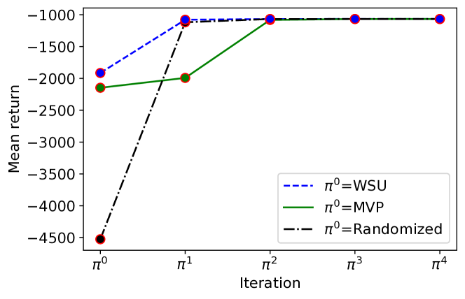
Figure 1: Mean Returns of CADP with Different Initial Policies at Different Iterations

Second, Table 1 summarizes the returns, or solution quality, of the algorithms on HIV domain for horizon length $T=15$ and other domains for horizon length $T=50$ evaluated on the test set. Table 2 summarizes the standard deviation of returns of the algorithms on five domains. The results for other time horizons, which are reported in the appendix, are very similar. The algorithm “Oracle” describes an algorithm that knows that the true model and its returns are the means of each model’s optimal values. Note that Oracle’s return may be a lose upper bound on the best possible return. If the runtime of a method is greater than 900 minutes, the method is considered to fail to find a solution and is marked with ‘–’. BasicPOMCP and QMDP approximate solvers fail to find solutions on domains POP, POPS, and INV.

Table 1: Mean return $\rho(\pi)$ on the Test Set of Policies $\pi$ Computed by Each Algorithm. HIV Values are in 1000s.

Algorithm	RS	POP	POPS	INV	HIV
CADP	204	-361	-1067	323	42
WSU	203	-542	-1915	323	42
MVP	201	-704	-2147	323	42
Mirror	181	-1650	-3676	314	42
Gradient	203	-542	-1915	323	42
MixTS	167	-1761	-2857	327	-1
QMDP	190	–	–	–	40
POMCP	58	–	–	–	30
Oracle	210	-168	-882	332	53

Table 2: Standard deviation of returns of algorithms. HIV values are in 1000s.

Algorithm	RS	POP	POPS	INV	HIV
CADP	96	1081	1986	47	11
WSU	98	1346	3119	49	11
MVP	89	2018	3577	48	11
Mirror	69	2150	4494	52	11
Gradient	98	1346	3119	49	11
MixTS	223	4398	5454	58	26
QMDP	213	-	-	-	64
POMCP	72	-	-	-	55
Oracle	93	1032	1868	47	14

Run-time

Table 3 summarizes the runtime of several algorithms on the domains for horizon length $T=50$. All algorithms were executed on a Ubuntu 20.04 with 3.0 GHz Intel processor and 32 GB of RAM. BasicPOMCP and QMDP approximate solvers fail to compute a policy on domains POP, POPS, and INV in a reasonable time. MVP runs fastest. MixTS runs slower than MVP but faster than other algorithms. The CADP method needs several iterations to get the policy that achieves the local maximum. As we expected, the time taken by CADP to solve these instances is several times as much as WSU. How quickly the CADP converges depends on the length of the time horizon and the number of iterations performed.

Table 3: Run-times to compute a policy $\pi$ in minutes.

Algorithm	RS	POP	POPS	INV	HIV
CADP	0.29	69.66	5.39	0.88	0.0053
WSU	0.08	33.65	0.95	0.45	0.0016
MVP	0.05	27.60	0.36	0.22	0.0002
Mirror	1.06	67.88	4.44	2.88	0.0111
Gradient	0.46	40.78	1.52	0.79	0.0042
MixTS	0.07	28.06	0.59	0.34	0.0018
QMDP	712	–	–	–	0.7100
POMCP	68	–	–	–	0.2066

Discussion

Our results show that CADP consistently achieves the best or near-best return in all domains and time horizons. This is remarkable because it only looks for Markov policies, whereas several other algorithms consider the richer space of history-dependent policies. The computational penalty that CADP incurs compared to just solving the average model, as done by MVP, is only a factor of 3-10. In comparison, state-of-the-art POMDP solvers were unable to solve most of the domains within a factor of 100 of CADP’s runtime.

Let us take a closer look at the performance of the algorithms for a horizon $50$ on domain POPS. The runtime of WSU is $0.95$ minutes, but the return that WSU obtains is $-1915$. The runtime taken by CADP is $5.6$ times as much as WSU, but the return for CADP is -1067, which is significantly greater than what WSU achieves. MixTS is a sampling-based algorithm that is guaranteed to perform well over long horizons but has no guarantees for short horizons. However, this assumption may not hold in this domain, which could cause MixTS to perform poorly. The mirror descent algorithm and CADP obtain the same return on the domain HIV, but CADP performs significantly better than the mirror descent algorithm on other domains. Therefore, CADP outperforms those approaches with some runtime penalty.

7 Conclusions and Future Work

This paper proposes a new efficient algorithm, CADP, which combines a coordinate ascent method and dynamic programming to solve MMDPs. CADP incorporates adjustable weights into the MMDP and adjusts the model weights each iteration to optimize the deterministic Markov policy to the local maximum. Our experiment results and theoretical analysis show that CADP performs better than existing approximation algorithms on several benchmark problems. The only drawback of CADP is that it needs several iterations to obtain a converged policy and increases the computational complexity. In terms of future work, it would be worthwhile to scale up CADP to value function approximation and consider richer soft-robust objectives. It also would be worthwhile to design algorithms that add limited memory to the policy to compute simple history-dependent policies.

Acknowledgements

We thank the anonymous reviewers for their comments. This work was supported, in part, by NSF grants 2144601 and 1815275.

References

- Agarwal et al. [2021] Alekh Agarwal, Sham M Kakade, Jason D Lee, and Gaurav Mahajan. On the theory of policy gradient methods: optimality, approximation, and distribution shift. The Journal of Machine Learning Research, 22(1):4431–4506, 2021.
- Ahluwalia et al. [2021] Vinayak S Ahluwalia, Lauren N Steimle, and Brian T Denton. Policy-based branch-and-bound for infinite-horizon multi-model Markov decision processes. Computers & Operations Research, 126:105–108, 2021.
- Bala and Mauskopf [2006] Mohan V Bala and Josephine A Mauskopf. Optimal assignment of treatments to health states using a Markov decision model. Pharmacoeconomics, 24(4):345–354, 2006.
- Behzadian et al. [2021] Bahram Behzadian, Reazul Hasan Russel, Marek Petrik, and Chin Pang Ho. Optimizing percentile criterion using robust MDPs. In International Conference on Artificial Intelligence and Statistics (AISTATS). PMLR, 2021.
- Ben-Tal et al. [2009] Aharon Ben-Tal, Laurent El Ghaoui, and Arkadi Nemirovski. Robust optimization. Princeton University Press, 2009.
- Bertsekas [2016] Dimitri P Bertsekas. Nonlinear Programming. Athena Scientific, 3rd edition, 2016.
- Bertsimas et al. [2018] Dimitris Bertsimas, John Silberholz, and Thomas Trikalinos. Optimal healthcare decision making under multiple mathematical models: application in prostate cancer screening. Health Care Management Science, 21(1):105–118, 2018.
- Bhandari and Russo [2021] Jalaj Bhandari and Daniel Russo. On the linear convergence of policy gradient methods for finite MDPs. In International Conference on Artificial Intelligence and Statistics (AISTATS). PMLR, 2021.
- Boucherie and Van Dijk [2017] Richard J Boucherie and Nico M Van Dijk. Markov decision processes in practice. Springer, 2017.
- Buchholz and Scheftelowitsch [2019a] Peter Buchholz and Dimitri Scheftelowitsch. Light robustness in the optimization of Markov decision processes with uncertain parameters. Computers and Operations Research, 108:69–81, 2019a.
- Buchholz and Scheftelowitsch [2019b] Peter Buchholz and Dimitri Scheftelowitsch. Computation of weighted sums of rewards for concurrent MDPs. Mathematical Methods of Operations Research, 89(1):1–42, 2019b.
- Chen et al. [2017] Qiushi Chen, Turgay Ayer, and Jagpreet Chhatwal. Sensitivity analysis in sequential decision models: a probabilistic approach. Medical Decision Making, 37(2):243–252, 2017.
- Delage and Mannor [2010] Erick Delage and Shie Mannor. Percentile optimization for Markov decision processes with parameter uncertainty. Operations Research, 58(1):203–213, 2010.
- Derman et al. [2018] Esther Derman, Daniel Mankowitz, Timothy A Mann, and Shie Mannor. Soft-robust actor-critic policy-gradient. In Uncertainty in Artificial Intelligence (UAI), 2018.
- Ferrer-Mestres et al. [2020] Jonathan Ferrer-Mestres, Thomas G Dietterich, Olivier Buffet, and Iadine Chades. Solving K-MDPs. In International Conference on Automated Planning and Scheduling (ICAPS), volume 30, 2020.
- Givan et al. [2000] Robert Givan, Sonia Leach, and Thomas Dean. Bounded-parameter Markov decision processes. Artificial Intelligence, 122(1):71–109, 2000.
- Goyal and Grand-Clement [2022] Vineet Goyal and Julien Grand-Clement. Robust Markov decision processes: beyond rectangularity. Mathematics of Operations Research, 48:203–226, 2022.
- Hallak et al. [2015] Assaf Hallak, Dotan Di Castro, and Shie Mannor. Contextual Markov decision processes. arXiv:1502.02259v1, 2015.
- Ho et al. [2021] Chin Pang Ho, Marek Petrik, and Wolfram Wiesemann. Partial policy iteration for L1-robust Markov decision processes. Journal of Machine Learning Research, 22(1):12612–12657, 2021.
- Hong et al. [2022] Joey Hong, Branislav Kveton, Manzil Zaheer, Mohammad Ghavamzadeh, and Craig Boutilier. Thompson sampling with a mixture prior. In International Conference on Artificial Intelligence and Statistics (AISTATS). PMLR, 2022.
- Iyengar [2005] Garud N Iyengar. Robust dynamic programming. Mathematics of Operations Research, 30(2):257–280, 2005.
- Kaelbling et al. [1998] Leslie Pack Kaelbling, Michael L Littman, and Anthony R Cassandra. Planning and acting in partially observable stochastic domains. Artificial Intelligence, 101(1-2):99–134, 1998.
- Kochenderfer et al. [2022] Mykel J Kochenderfer, Tim A Wheeler, and Kyle H Wray. Algorithms for decision making. MIT press, 2022.
- Lattimore and Szepesvári [2020] Tor Lattimore and Csaba Szepesvári. Bandit algorithms. Cambridge University Press, 2020.
- Littman et al. [1995] Michael L Littman, Anthony R Cassandra, and Leslie Pack Kaelbling. Learning policies for partially observable environments: Scaling up. In Machine Learning Proceedings. 1995.
- Lobo et al. [2020] Elita A Lobo, Mohammad Ghavamzadeh, and Marek Petrik. Soft-robust algorithms for batch reinforcement learning. arXiv preprint arXiv:2011.14495, 2020.
- Mannor et al. [2016] Shie Mannor, Ofir Mebel, and Huan Xu. Robust MDPs with k-rectangular uncertainty. Mathematics of Operations Research, 41(4):1484–1509, 2016.
- Nilim and El Ghaoui [2005] Arnab Nilim and Laurent El Ghaoui. Robust control of Markov decision processes with uncertain transition matrices. Operations Research, 53(5):780–798, 2005.
- Petrik and Luss [2016] Marek Petrik and Ronny Luss. Interpretable policies for dynamic product recommendations. In Uncertainty in Artificial Intelligence (UAI), 2016.
- Petrik and Russel [2019] Marek Petrik and Reazul Hasan Russel. Beyond confidence regions: tight bayesian ambiguity sets for robust MDPs. Advances in Neural Information Processing Systems (NeurIPS), 32, 2019.
- Puterman [2014] Martin L Puterman. Markov decision processes: discrete stochastic dynamic programming. John Wiley & Sons, 2014.
- Satia and Lave [1973] Jay K Satia and Roy E Lave. Markovian decision processes with uncertain transition probabilities. Operations Research, 21:728–740, 1973.
- Silver and Veness [2010] David Silver and Joel Veness. Monte-carlo planning in large pomdps. Advances in Neural Information Processing systems (NIPS), 2010.
- Steimle et al. [2018] Lauren N Steimle, David L Kaufman, and Brian T Denton. Multi-model Markov decision processes. Technical report, Optimization-online, 2018.
- Steimle et al. [2021a] Lauren N Steimle, Vinayak S Ahluwalia, Charmee Kamdar, and Brian T Denton. Decomposition methods for solving Markov decision processes with multiple models of the parameters. IISE Transactions, 53(12):1295–1310, 2021a.
- Steimle et al. [2021b] Lauren N Steimle, David L Kaufman, and Brian T Denton. Multi-model Markov decision processes. IISE Transactions, 53(10):1124–1139, 2021b.
- Strehl and Littman [2008] Alexander L Strehl and Michael L Littman. An analysis of model-based interval estimation for Markov decision processes. Journal of Computer and System Sciences, 74(8):1309–1331, 2008.
- Sutton and Barto [2018] Richard S Sutton and Andrew G Barto. Reinforcement learning: an introduction. The MIT Press, 2018.
- Vlassis et al. [2012] Nikos Vlassis, Michael L Littman, and David Barber. On the computational complexity of stochastic controller optimization in POMDPs. ACM Transactions on Computation Theory, 4(4):1–8, 2012.
- Wiesemann et al. [2013] Wolfram Wiesemann, Daniel Kuhn, and Berç Rustem. Robust Markov decision processes. Mathematics of Operations Research, 38(1):153–183, 2013.
- Xu and Mannor [2012] Huan Xu and Shie Mannor. Distributionally robust Markov decision processes. Mathematics of Operations Research, 37(2):288–300, 2012.