CONGO: Compressive Online Gradient Optimization with Application to Microservices Management

Abstract

We address the challenge of online convex optimization where the objective function’s gradient exhibits sparsity, indicating that only a small number of dimensions possess non-zero gradients. Our aim is to leverage this sparsity to obtain useful estimates of the objective function’s gradient even when the only information available is a limited number of function samples. Our motivation stems from distributed queueing systems like microservices-based applications, characterized by request-response workloads. Here, each request type proceeds through a sequence of microservices to produce a response, and the resource allocation across the collection of microservices is controlled to balance end-to-end latency with resource costs. While the number of microservices is substantial, the latency function primarily reacts to resource changes in a few, rendering the gradient sparse. Our proposed method, CONGO (Compressive Online Gradient Optimization), combines simultaneous perturbation with compressive sensing to estimate gradients. We establish analytical bounds on the requisite number of compressive sensing samples per iteration to maintain bounded bias of gradient estimates, ensuring sub-linear regret. By exploiting sparsity, we reduce the samples required per iteration to match the gradient’s sparsity, rather than the problem’s original dimensionality. Numerical experiments and real-world microservices benchmarks demonstrate CONGO’s superiority over multiple stochastic gradient descent approaches, as it quickly converges to performance comparable to policies pre-trained with workload awareness.

1 Introduction

Online convex optimization (OCO) has become increasingly significant in managing various distributed applications, such as web caching, advertisement placement, portfolio selection, and recommendation systems. These applications entail an unknown, convex system cost function $f_{t}(x_{t})$ which is time-varying and depends on a $d$-dimensional control denoted $x_{t}$ that the user can choose in an online manner. Of particular interest to us are systems that exhibit three critical attributes: (i) the function $f_{t}(\cdot)$ and its gradient are unknown, with acquiring measurements for a given allocation $x_{t}$ being costly; (ii) the gradient of $f_{t}(\cdot)$ manifests sparsity, where locally only a few dimensions of $x_{t}$ significantly affect $f_{t}(\cdot)$; and (iii) the evolution of $f_{t}(\cdot)$ occurs slowly, allowing for multiple measurements within the time step $[t,t+1]$ before changes occur. Our objective is to devise an efficient online gradient descent strategy tailored to address these systems.

Our study is motivated by the necessity to autoscale resources to ensure low-latency response times for cloud applications, organized into microservices, each running in containers. These applications can be modeled as a queueing networks, where each microservice consists of a queue and server and requests traverse a sequence of microservices before exiting. The average latency at a node is convex in both the workload and server resources (like CPU, memory, etc.), which are dynamically allocated. The price of server resources is often on a per-unit basis, and hence is linear in the server resources allocated. The goal of autoscaling is to minimize a cost function consisting of a linear combination of average latency and the price of resources used. Workload composition and intensity change over time, making the latency function at each node unknown and variable. As we show in Section 3, these applications exhibit the three critical attributes mentioned above, and hence, online gradient descent is suitable for our cost minimization problem.

Our approach is informed by work on gradient estimation via simultaneous perturbation  [24] and compressive sensing for gradient estimation [3], where multiple dimensions of the input are perturbed simultaneously to obtain noisy linear combinations of the desired gradients. We develop an online learning algorithm, Compressive Online Gradient Optimization (CONGO), which estimates gradients using a limited number of such perturbations. These gradient estimates are biased, and one of our key analytical results is to find the number of samples sufficient to limit the bias of the estimates such that low regret is possible. We develop sub-linear finite-time regret bounds for online gradient descent using CONGO. Our analysis shows that both the number of samples needed and the dominant terms of the regret bound are proportional to the sparsity of the gradient, which is significantly lower than the dimensionality of the objective function. This implies that CONGO is effective at exploiting the underlying sparsity, both in terms of optimality of its decisions and in sampling costs incurred.

We apply CONGO to autoscaling microservices, focusing on scaling CPU resources, as they have been demonstrated to be most crucial for microservices [28; 22]. We begin with a queueing network simulation, and show both the effectiveness of stochastic gradient descent with simultaneous perturbations (SGDSP) and the benefit obtained by exploiting sparsity using CONGO. We then deploy CONGO for a popular microservice benchmark application [11]. We compare CONGO against multiple alternative schemes, and show that it approaches the performance of the optimal reinforcement learning (RL) baseline within 12-15 iterations, even as the load varies, and maintains an average cost as low as or lower than the best gradient descent alternative.

Related Work: We provide an overview of related work here, with details in Appendix A.

Over the years, online convex optimization with a few evaluation points has been used to study environments where the cost varies sequentially over time,  [9; 4] among many others. The performance metric for this problem is typically the static regret based on the best action in hindsight, see  [12] for a good introduction to the topic. Several works have not only been able to characterize information theoretic minimax regret bounds under bandit feedback, see for example  [17] but have also provided algorithms that can achieve these bounds  [18; 1; 15; 27] to name a few. Our work is distinguished by the fact that our control is fixed over a period but we are free to take samples from the process in the local neighborhood of this control.

Such scenarios are frequently encountered in microservice applications (see  [14]) where significant resource allocation changes must be made carefully but one may measure the quality of service continuously over a period. We provide a detailed overview of both the microservice literature as well as the pitfalls of the various approaches towards resource allocation in Appendix A. A common theme in the resource allocation problem is the curse of dimensionality that stems from a large number of resources and resource flows when considering microservices. Bearing this in mind we wish to use simultaneous perturbation stochastic approximation (SPSA) proposed in [24] in order to compute gradient approximations while avoiding the problem of dimensionality. A comprehensive examination of the method with examples is provided in [2]. On top of this, the assumption of sparse gradients in our system model allows us to apply the theory of compressive sensing. Since its inception due to the seminal paper  [5], this theory has been used in signal processing  [8] for the sparse recovery of signals. The main value of compressive sensing is that the number of measurements required to obtain a suitable approximation of an $s$-sparse vector (defined in 2) can be made to scale only logarithmically with the dimensionality $d$ of the vector.

2 Problem formulation

System model and sequence of events: We consider an online learning problem over $T$ rounds indexed from $1$ to $T$. At the start of each round $t$ the controller must choose a $d$ dimensional control $x_{t}\in\mathcal{K}$ where $\mathcal{K}\subset\mathbb{R}^{d}$ is known. We would like to emphasize that we are in a high dimensional regime such that $d$ is a large value. Next, an adversary chooses a differentiable convex function $f_{t}:\mathbb{R}^{d}\rightarrow\mathbb{R}$ and the controller receives the cost $f_{t}(x_{t})$. The controller is unaware of the function $f_{t}$, however, we may acquire samples of $f_{t}$ in a local vicinity of $f_{t}(x_{t})$ to use alongside the observed cost. We do this by perturbing the control to $\tilde{x}_{t}\in\mathbb{R}^{d}$ and observing $f_{t}(\tilde{x}_{t})$. Over a given round, the player may gather $k$ such samples for its computational purposes. Note that in our constrained optimization setting, we permit the extra samples used for gathering information on $\tilde{\nabla}f_{t}(x_{t})$ to lie outside of $\mathcal{K}$ so long as they remain close to $x_{t}$ in expectation. The timeline of events can be found in Figure 1.

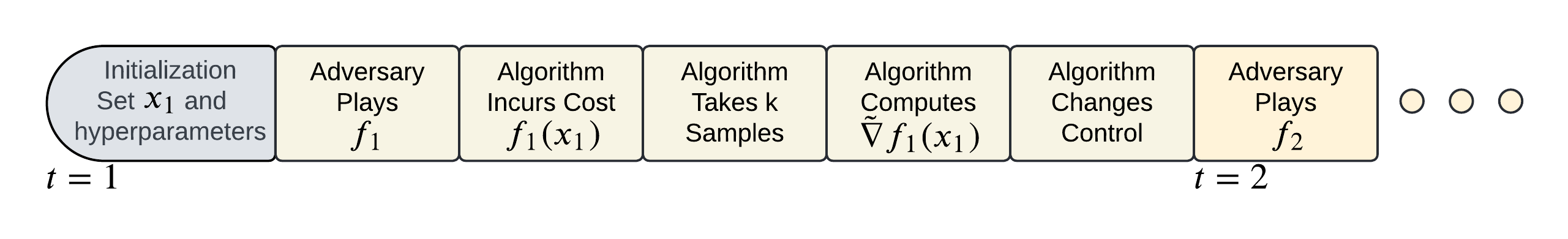
Figure 1: Timeline of events.

Control strategy: In this work, we will examine an online projected gradient descent algorithm where the samples retrieved are used to estimate a noisy gradient. In particular, at the end of round $t$, we use the $k$ samples and the observed cost $f_{t}(x_{t})$ to compute an estimate $\tilde{\nabla}f_{t}(x_{t})$. The online gradient descent algorithm dictates that we should use

$$x_{t+1}=\underset{x\in\mathcal{K}}{\textrm{argmin}}||x-(x_{t}-\eta_{t}\tilde{\nabla}f_{t}(x_{t}))||_{2}$$

as the control for our next time step. Here $\eta_{t}$ is a predetermined step-size chosen by the controller.

Assumptions: Our setting uses two key assumptions on the constraint set $\mathcal{K}$ and the observed functions.

Assumption 1 (Constraint Set Properties).

The set $\mathcal{K}\subset\mathbb{R}^{d}$ satisfies the following properties:

• $\mathcal{K}$ is compact and convex

• $\underset{x\in\mathcal{K}}{\sup}||x||_{2}\leq R$.

An important way in which our setting differs from standard online convex optimization is that we make an assumption about the sparsity of $\nabla f_{t}$. We define sparsity as follows:

Definition 1 (Sparsity).

The support of a vector $x\in\mathbb{R}^{d}$ is:

$$supp(x):=\{j\in\{1,2,\dots d\}:x(j)\neq 0\}.$$ (1)

We call a vector $x$ $s$-sparse if $|supp(x)|\leq s$.

Our overall constraints on the set of functions the adversary can choose from are summarized below:

Assumption 2 (Function Properties).

Let $\mathcal{F}$ denote the set of all functions $f$ which satisfy the following properties:

• $f$ is convex, $L_{f}$-Lipschitz, and $L$-smooth

• $\nabla f(x)$ is $s$-sparse.

• $||\nabla^{2}f||_{2}\leq B_{H}<\infty$

For each time $t\in[1,T]$, we assume our functions $f_{t}$ are chosen such that $f_{t}\in\mathcal{F}$.

As mentioned in Section 1, the significance of the sparsity assumption is that an algorithm may be able to exploit this sparsity such that the number of samples it requires and the overall regret has little or no dependence on $d$. The challenge, of course, is that we do not know a priori which dimensions of $\nabla f_{t}$ are nonzero at our current control point, and this can change at every round.

Performance Metric: Our performance metric of interest is the adversarial regret at the end of $T$ rounds, which measures the difference in the cost accumulated over the $T$ rounds with that of the best fixed control point in hindsight. In what follows we shall formally define the adversarial regret.

Definition 2 (Adversarial Regret).

Given a sequence of convex functions $\{f_{t}\}_{t=1}^{T}$ satisfying 2, our objective is to minimize the following quantity which we call the regret:

$$R(T):=\max_{f_{\tau}\in\mathcal{F},\tau=1,2,\dots T}\left(\sum_{t=1}^{T}f_{t}(x_{t})-\min_{x^{\star}}\sum_{t=1}^{T}f_{t}(x^{\star})\right)$$ (2)

3 Motivating example

In this section, we elaborate upon the microservice autoscaling problem introduced in Section 1, and how it fits into our problem formulation. We define the (end-to-end) latency of a job to be the delay between the arrival time of the job and the time when it has been processed. Note that under normal operating conditions the average latency at a single microservice is convex in both the workload and the service rate, and hence the end-to-end latency will be as well. We call the distribution of incoming jobs, along with the overall arrival rate, the workload. The arriving jobs are time-sensitive - hence, each new job is expected to be processed as soon as it arrives. To minimize operating costs, we would like to only pay for the resources that are strictly needed for jobs to be processed with a latency acceptable to users.

If we let the control $x_{t}$ denote the quantity of resources allocated to each microservice at any time $t$ (where each dimension of $x_{t}$ corresponds to the resources allocated to a specific microservice), then we can define our objective function in terms of $x_{t}$ as

$$f_{t}(x_{t})=L(\lambda_{t},x_{t})+w\sum_{i=1}^{d}[x_{t}]_{i}$$ (3)

where $w$ denotes the price per unit of computing resource allocated to a microservice (assumed to be the same for all microservices), and $L(\lambda_{t},x_{t})$ is the expectation (taken over the workload $\lambda_{t}$) of the end-to-end latency which jobs experience when the system is using the allocation $x_{t}$. The elements of $w$ reflect the per unit resource price that must be paid to a cloud resource provider (e.g. Amazon Web Services) to reserve resources for each microserivice. In practice, we are only able to sample the end-to-end latencies experienced by a finite number of jobs passing through the system to reduce the measurement overhead. Consequently, we use the sample mean of the measured latencies to approximate $L(\lambda_{t},\cdot)$ and perform stochastic gradient descent using those observations.

We now motivate the sparsity in large-scale heterogeneous microservices. Suppose only a small fraction of all jobs are processed by a certain microservice. In that case, slightly changing the resources of such a microservice will not significantly impact $L(\lambda_{t},x_{t})$ due to the relatively small contribution that the affected jobs make. This means that $\nabla_{x}L(\lambda_{t},x_{t})$ will be much smaller along the dimension corresponding to that microservice compared to heavily trafficked microservices. On the other hand, if there is a bottleneck present somewhere in the network of microservices, then increasing the service rate for any of the microservices feeding into the bottleneck will not impact the end-to-end latency since it will simply result in queue build-up at the bottleneck. This means that the dimensions of $\nabla_{x}L(\lambda_{t},x_{t})$ corresponding to those microservices will be close to 0. These facts suggest that under many different workloads and allocation levels, $\nabla_{x}L(\lambda_{t},x_{t})$ will be sparse, as per Definition 1, or at least approximately sparse. Thus, our strategy for solving the microservices autoscaling problem consists of using compressive sensing to get a good estimate of $\nabla_{x}L(\lambda_{t},x_{t})$ without too many measurements, calculating the resulting estimate of $\nabla f_{t}(x_{t})$ (since $w$ is known by the controller), and using that gradient estimate to run an algorithm like projected stochastic gradient descent.

4 Algorithm

In order to take a number of measurements depending mainly on $s$ and transform it into an estimate of $\nabla f_{t}(x_{t})\in\mathbb{R}^{d}$, we must combine the methods of SPSA and compressive sensing; we provide the necessary background here and the full details in Appendix A.

Simultaneous Perturbation: SPSA, due to [24], operates as follows: First, generate a sequence of $d$ i.i.d. Rademacher random variables, $\{\Delta_{j}\}_{j=1}^{d}$. Next, generate, a perturbation vector $\Delta:=\sum_{j=1}^{d}e_{j}\Delta_{j}$ with $e_{j}$ being the $j$th unit vector. Finally, compute the gradient estimate as follows:

$$\frac{f(x+\delta\Delta)-f(x)}{\delta\Delta_{j}}\approx\frac{\partial f(x)}{\partial x_{i}}+\sum_{i\neq j}\frac{\partial f(x)}{\partial x_{i}}\frac{\Delta_{i}}{\Delta_{j}}$$

Compressive Sensing: Results in compressive sensing (see Appendix A) tell us that given measurements of the form $\textbf{{{A}}}\nabla f(x)+\eta$ where A is a suitable random measurement matrix and $\eta$ is bounded measurement noise, an approximation $\tilde{\nabla}f(x)$ can be obtained as the result of an $l1$-minimization problem such that $||\tilde{\nabla}f(x)-\nabla f(x)||_{2}$ is bounded by a quantity proportional to $||\eta||_{2}$. What enables CONGO to exploit sparsity through compressive sensing is the fact that these measurements can be obtained through a SPSA-like method. This is seen in the gradient estimation method provided by [3]: if the perturbation vector is ${\textbf{{{A}}}}^{T}\Delta$ and $\Delta$ is a vector of $m$ Rademacher random variables, then SPSA provides measurements $y=\textbf{{{A}}}\nabla f(x)+\eta$ where $\eta$ is nearly zero-mean noise.

Overall, our algorithm can be divided into an outer loop that performs projected gradient descent and an inner loop that performs the gradient estimation, by applying algorithm 1 in [3] for recovering a sparse approximation to the gradient in the presence of measurement noise. The full pseudocode for CONGO is provided in Algorithm 1.

While Algorithm 1 in [3] only requires slight modification to be applied in our particular OCO setting and obtain meaningful regret bounds, our analysis differs greatly from theirs since they focus on offline gradient descent and only prove convergence to a small neighborhood of some local minimum of the objective function. On the other hand, we are considering a setting where the objective function changes after each gradient descent step and consider how large $k$ must be in order to obtain a good enough estimate of the gradient on each round to prevent regret from accumulating too quickly.

Algorithm 1 CONGO: Compressive Online Gradient Optimization

0:  Constraint set $\mathcal{K}$, Horizon $T$, Parameters $(\eta_{t})_{t=1}^{T}$, $m$, $k$, $\delta$, $\gamma$

  $\gamma\leftarrow(2mK+1)\delta$ $\triangleright$ Noise bound

  for $t=1,2,\cdots,T$ do

     Observe cost $f_{t}(x_{t})$ and incur regret $f_{t}(x_{t})-f_{t}(x^{*})$

     $\textbf{{{A}}}\leftarrow$ random $m\times d$ matrix with i.i.d. standard normal entries $\triangleright$ Measurement Matrix

     for $l=1,2,\cdots,k$ do

        $\Delta^{l}\leftarrow$ random $m$-dimensional vector of Rademacher random variables

        Query at point $x_{t}+\delta{\textbf{{{A}}}}^{T}\Delta^{l}$ to get $f_{t}(x_{t}+\delta{\textbf{{{A}}}}^{T}\Delta^{l})$

        $\beta^{l}\leftarrow f_{t}(x_{t}+\delta{\textbf{{{A}}}}^{T}\Delta^{l})-f_{t}(x_{t})$ $\triangleright$ Finite difference

        for $i=1,2,\cdots,m$ do

           $y_{i}^{l}\leftarrow\frac{\beta^{l}}{\delta\Delta_{i}^{l}}$ $\triangleright$ Compute observation for each row of A

        end for

     end for

     $y\leftarrow\left(\frac{1}{k}\sum_{l=1}^{k}y_{1}^{l},\cdots,\frac{1}{k}\sum_{l=1}^{k}y_{m}^{l}\right)$ $\triangleright$ Average over observations

     if There exists a feasible solution $z^{*}$ for

$$\min||z||_{1}\textrm{ }\textrm{subj. to}\textrm{ }||\textbf{{{A}}}z-y||_{2}\leq\gamma\textrm{ and }||z||_{2}\leq L_{f}+\frac{2\gamma}{\tau}$$

 then

        $\tilde{\nabla}f_{t}(x_{t})\leftarrow z^{*}$ $\triangleright$ Gradient estimate from Compressive Sensing

     else

        $\tilde{\nabla}f_{t}(x_{t})\leftarrow 0$ $\triangleright$ In case of gradient estimation failure, maintain current control

     end if

     $x_{t+1}\leftarrow\underset{x\in\mathcal{K}}{\textrm{argmin}}||x-(x_{t}-\eta_{t}\tilde{\nabla}f_{t}(x_{t}))||_{2}$ $\triangleright$ Gradient Descent Update

  end for

The following result gives a probabilistic guarantee on the accuracy of the gradient estimate obtained using compressive sensing. It establishes that given enough samples and an appropriate choice of $\gamma$ in the recovery procedure, one can achieve a bound on the error in the gradient estimate which holds with any desired probability. This result is thus crucial for the proof of our main result, Theorem 1.

Lemma 1 (Theorem 4 of [3]).

Let $f:\mathbb{R}^{d}\mapsto\mathbb{R}$ be a continuously differentiable function with bounded sparse gradient. Then for $m\in\mathbb{N}$ such that it satisfies

$$\frac{m^{2}}{m+1}\geq 2s\left(\sqrt{\log\left(\frac{ed}{s}\right)}+\sqrt{\frac{\log(\epsilon^{-1})}{s}}+\frac{\tau}{\sqrt{s}}\right)^{2},$$

$0<\epsilon<<\frac{1}{m}$, $\delta>0$, and $\tau>0$, $\nabla f(x)$ can be estimated by a sparse vector $\tilde{\nabla}f(x)$ such that with probability at least $1-\epsilon m$,

$$||\tilde{\nabla}f(x)-\nabla f(x)||_{2}<\frac{2\gamma}{\tau}$$ (4)

where $\gamma>2m\mathcal{O}\left(\delta\right)$, and the $\mathcal{O}\left(\delta\right)$ term is bounded above by $K\delta$ where $K=B_{H}||\textbf{{{A}}}||_{2}$. In particular, the number of samples $k$ to average over must be at least $\frac{2m^{2}(m-1)G^{2}}{\gamma^{2}}\log(\frac{2}{\epsilon})$ where $G\geq\sup_{i}|\langle\nabla f(x),a_{i}\rangle|$, with $a_{i}$ being the $i$th row of A.

While the recovery process for our algorithm features the additional constraint that $||z||_{2}\leq L_{f}+\frac{2\gamma}{\tau}$ which [3] did not consider, it does not affect the applicability of this result to our algorithm. To see this, note that under any outcome where the solution to the $l1$-minimization problem without the second constraint satisfies (4), we know that

$$||\tilde{\nabla}f(x)||_{2}<\frac{2t}{\tau}+||\nabla f(x)||_{2}\leq\frac{2t}{\tau}+L_{f}$$

by the triangle inequality, and hence the second constraint is immediately satisfied. This second constraint is primarily technical and it does not play any significant role in the practical implementation of CONGO. As Lemma 2 will show, Lemma 1 can be translated to a bound on $\mathbb{E}\left[\left\lVert\tilde{\nabla}f(x)-\nabla f(x)\right\rVert_{2}^{2}\right]$ and hence, by Jensen’s inequality, a bound on the bias of the gradient estimate.

5 Theoretical results

We now state the key lemma for our proof of CONGO’s regret bound.

Lemma 2.

Let $f$ satisfy all the conditions of 2, and assume that we run the gradient estimation routine for some $\delta>0$, $\gamma>2mK\delta$, $0<\epsilon<1$, $\tau>0$, $k\geq 2m^{2}(m-1)G^{2}\gamma^{-2}\log\left(\frac{2}{\epsilon}\right)$ and $m=\left\lceil 2s\left(\sqrt{\log\left(\frac{ed}{s}\right)}+\sqrt{\frac{\log(\epsilon^{-1})}{s}}+\frac{\tau}{\sqrt{s}}\right)\right\rceil$ (where $K$ and $G$ are as defined in Lemma 1) at some point $x\in\mathcal{K}$ to obtain the estimate $\tilde{\nabla}f(x)$. Then

$$\mathbb{E}\left[\left\lVert\tilde{\nabla}f(x)-\nabla f(x)\right\rVert_{2}^{2}\right]\leq\left(\frac{2\gamma}{\tau}\right)^{2}+\left(\frac{2\gamma}{\tau}+2L_{f}\right)^{2}\epsilon m$$

Equipped with this bound on the gradient estimation error in expectation, we can use standard techniques to derive the regret that Algorithm 1 suffers in our online setting.

The following is the main theoretical result of our paper, where we bound the regret of our algorithm when the time horizon is known in advance. This result guarantees performance in the adversarial setting, and hence stochastically chosen functions chosen as well.

Theorem 1.

Under Assumptions 1 and 2, if we let $\gamma=(2mK+1)\delta$, $k=\left\lceil\frac{2m^{2}(m-1)G^{2}}{(2mK+1)^{2}}T\log(2T)\right\rceil$ (where $K$ and $G$ are as defined in Lemma 1), $\delta=\frac{1}{\sqrt{T}}$ and $\eta_{t}=\frac{1}{\sqrt{T}}\textrm{ }\forall t$, and furthermore we let

$$m=\left\lceil 2s\left(\sqrt{\log\left(\frac{ed}{s}\right)}+\sqrt{\frac{\log(T+1)}{s}}+\frac{\tau}{\sqrt{s}}\right)\right\rceil$$

with $\tau=\sqrt{\log(T+1)}$ then the regret of our algorithm after $T$ rounds scales as $\mathcal{O}\left(s\sqrt{\log(d/s)}\sqrt{T\log(T+1)}\right)$ (see proof for the full expression).

A few comments are now in order. First, the full dimensionality $d$ of the problem only appears in a logarithmic term, so the regret and $k$ are only weakly dependent upon it. This indicates the overwhelming advantage that our algorithm will have over those which do not exploit sparsity when $s<<d$. Second, while we do guarantee a regret within logarithmic factors of the order $\sqrt{T}$ regret which is optimal for the full-information OCO setting on smooth (not necessarily sparse) objective functions [12], the number of samples we use per round grows as order $T$. As seen in our theorem, there is a clear trade-off between the number of evaluations required and the regret we can incur. One might therefore ask what sort of regret guarantee we can get if we impose a stricter limit on the number of measurements of $f$ which can be taken in a round, say $k\leq T^{\frac{1}{q}}$ for some $q\geq 1$. The following corollary makes this trade-off explicit:

Corollary 1.

Suppose we restrict ourselves to choosing $k\leq T^{\frac{1}{q}}$ samples, for some $q\geq 1$. Then for any $0<p<\frac{1}{2q}$, by setting $\gamma=2m^{\frac{3}{2}}K\delta$ and $\delta=T^{-\frac{1}{2q}+p}$ in Algorithm 1 one can ensure a regret bound of order $T^{\frac{2q-1}{2q}}T^{\frac{3p}{2}}$. For very small $p$, when $q=1$ we approximately recover the $\mathcal{O}(\sqrt{T})$ regret guaranteed in Theorem 1, whereas when $q\to\infty$ (i.e. $k\to 1$) we get $\mathcal{O}\left(T\right)$ regret.

Note that if we set $q<1$, then the $\mathcal{O}(\sqrt{T})$ terms independent of $\delta$ and $\epsilon$ will dominate; hence, there is no benefit in choosing a value of $q$ smaller than $1$.

Finally, we bound the average magnitude of the deviations between the query points in a round and the actual control point for that round. First, note that $\mathbb{E}[{\textbf{{{A}}}}^{T}\Delta]=0$ since all random variables are independent and come from zero-mean distributions. The following theorem bounds the expected magnitude of the vector which defines the direction of a perturbation:

Theorem 2.

Let A and $\Delta$ be the random matrix and vector used to generate the perturbations in Algorithm 1. Then

$$\mathbb{E}\left[||{\textbf{{{A}}}}^{T}\Delta||_{2}\right]\leq\sqrt{md}$$

It follows that the average magnitude of the perturbations used in CONGO will be $\delta\sqrt{md}$. Since $m$ only scales as $\log(T)$, this will overall decrease as $T$ grows. Now, if we want to enforce a hard limit $B_{\Delta}$ on the magnitude of the perturbations, then we must set $\delta\leq\frac{B_{\Delta}}{\sqrt{md}}$ which means we cannot choose $\delta=\frac{1}{\sqrt{T}}$ as in Theorem 1 if $T<\frac{md}{B_{\Delta}^{2}}$. Modifying $\delta$ to satisfy the constraint will require the dependence upon $d$ for both the regret and $k$ to become greater, but it will not affect the scaling with respect to $T$ beyond logarithmic factors.

6 Benefits of compressive sensing

In what follows, we empirically demonstrate the superiority of the compressive sensing approach used by CONGO to standard SPSA (we use GDSP to denote the algorithm which performs gradient descent using standard SPSA) in the online setting under a relatively high degree of sparsity. We also show how CONGO compares to a projected gradient descent algorithm with full gradient information (denoted GD). In the numerical results presented in this section, we restrict the class of functions which the adversary can choose from to quadratic functions of the form

$$f(x)={x}^{T}Dx+{b}^{T}x+c$$

where $D$ is a diagonal matrix. Importantly, the vectors $\textrm{diag}(D)$ and $b$ are both $s$-sparse with identical support. This ensures that the gradient $\nabla f(x)=2Dx+b$ is $s$-sparse. The nonzero entries of $b$ are sampled from the standard normal distribution, and the nonzero entries of $D$ are sampled from the same distribution with the absolute value taken to ensure that $D$ is positive semidefinite. The value of $c$ is set to $10||b||_{1}$ so that we will have $f(x)\geq 0$ with very high probability. The constraint set in this case is a Euclidean ball of radius 1000 centered on the origin.

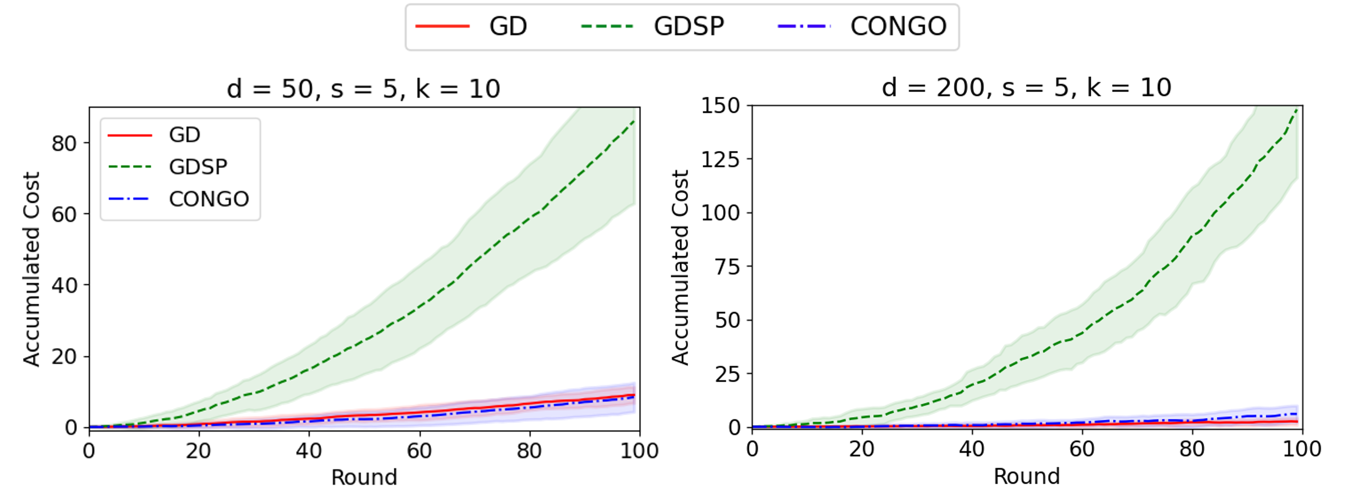
Figure 2: Comparison of accumulated costs: CONGO vs. baselines when the objective function is a quadratic with sparse gradient.

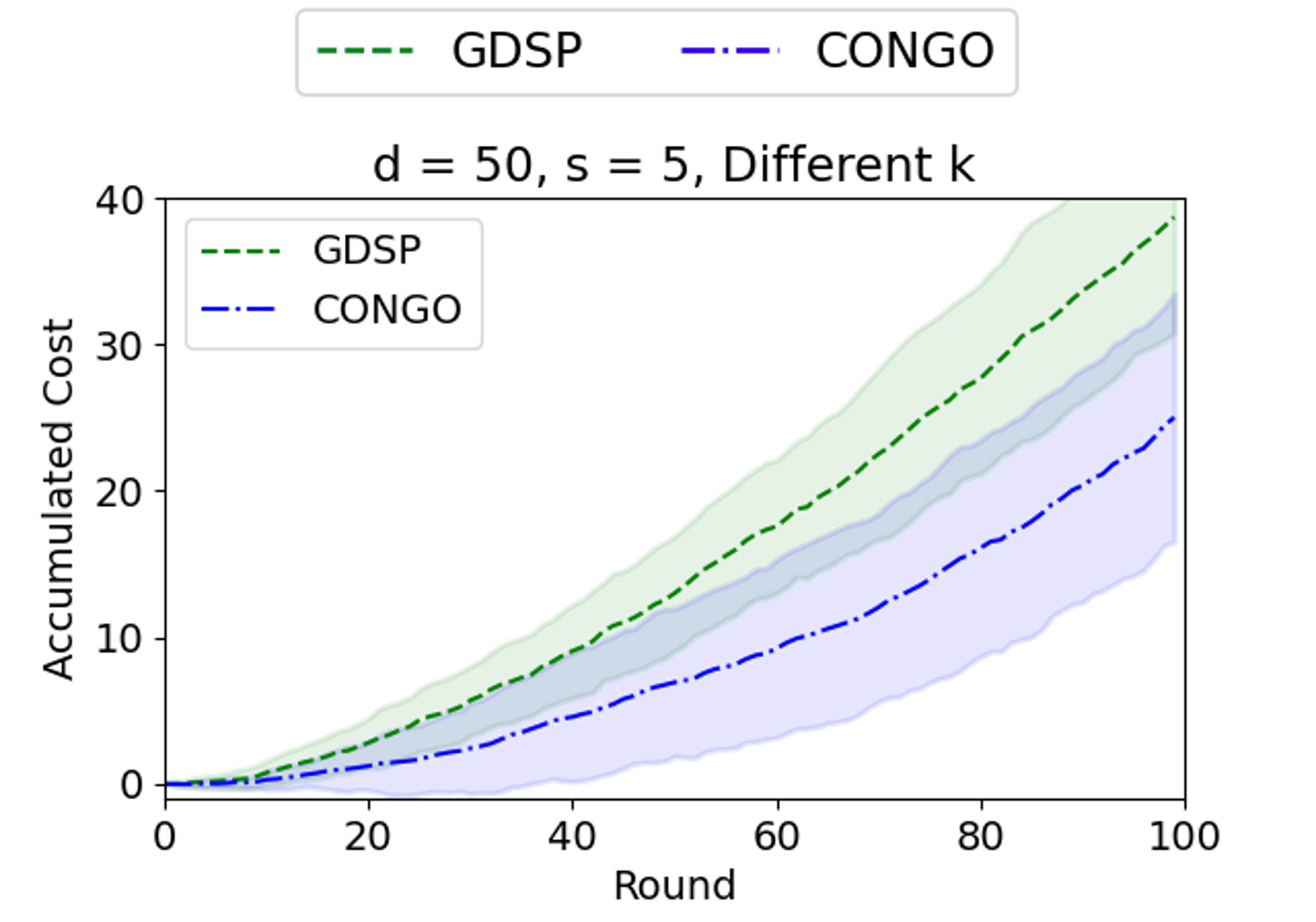
Figure 3: CONGO with $k=5$ outperforms GDSP with $k=20$.

Figure 3 shows the results for the three algorithms. More details on the parameters used for the experiment are given in Appendix C. For the 50-dimensional case, the plots are averaged over 50 random seeds, and for the 200-dimensional case, they averaged over 10 random seeds. We see that when given the same number of samples as GDSP (i.e. the same $k$), CONGO achieves a far lower regret which is comparable to that of exact gradient descent. Importantly, CONGO can outperform GDSP even when using fewer of samples (5 vs 20) as seen in Figure 3. The plots show one standard deviation of the cost at each round over all seeds.

7 Autoscaling of containerized microservices

We now discuss the application of CONGO to real-world usecases. In Section 7.1, we apply CONGO to a simulated Jackson Network representing a microservice application to show that its benefits can be reaped in many varied scenarios. Next, in Section 7.2, we deploy CONGO on a real-world microservice benchmark and demonstrate its practical benefits.

7.1 Jackson network simulation

Methodology: In the following experiments, we model a microservice application as a Jackson network [25], where each microservice is a single-server queue. The arrival of jobs follows a Poisson process, and the service rate of a server monotonically increases with the amount of resources allocated to the corresponding microservice. In particular, the service time experienced by a job is inversely related to the allocation for the given microservice: given an allocation $x$ the service time at the $i$th microservice is $\frac{1}{x_{i}+0.1}$. The cost function follows (3) but with $L(\cdot,\cdot)$ replaced by the sample average. In each simulation, we set $w=1$. To simulate the Jackson network, we use the Python package queueing-tool [16]. We consider two different Jackson network layouts - one with 15 and one with 50 microservices. A detailed description of the implementation can be found in Appendix C.

We conduct experiments for the two Jackson network layouts with three types of workloads: (i) fixed workload, (ii) fixed arrival rate with variable job types, and (iii) variable arrival rate with fixed job types.

Baselines: We compare CONGO against three gradient-descent baselines, which concretize the benefits observed in Section 6 for a general-purpose Jackson network. The first, Naive Stochastic Gradient Descent (NSGD), takes the naive approach of estimating the partial gradient along each dimension in isolation. The second, Stochastic Gradient Descent with Bayesian Optimization (SGDBO), is a simplified version of the stochastic gradient line Bayesian optimization algorithm proposed in [26]. The third is the stochastic variant of the GDSP algorithm mentioned in Section 6 (denoted SGDSP) since we do not have information of the function. See Appendix C for the implementation details. The results for each of these algorithms are averaged over five random seeds.

Results: We observe in Figure 5 that CONGO achieves the lowest final cost in all but one of the experiments, and it starts to perform better than the other algorithms within just 10 rounds. Note that SGDSP being the closest competitor shows that the use of simultaneous perturbations alone improves performance over more naive methods. We see that the gap between SGDSP and CONGO is larger when there are more microservices because of greater sparsity; the exception to this is the variable job type case for 50 microservices, where there are four job types (corresponding to 21 out of the 50 microservices) in use simultaneously during the transition between job distributions. We attribute CONGO’s failure to outperform SGDSP in this case to the lack of sparsity seen in the middle of the transition.

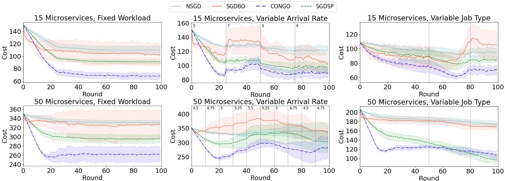
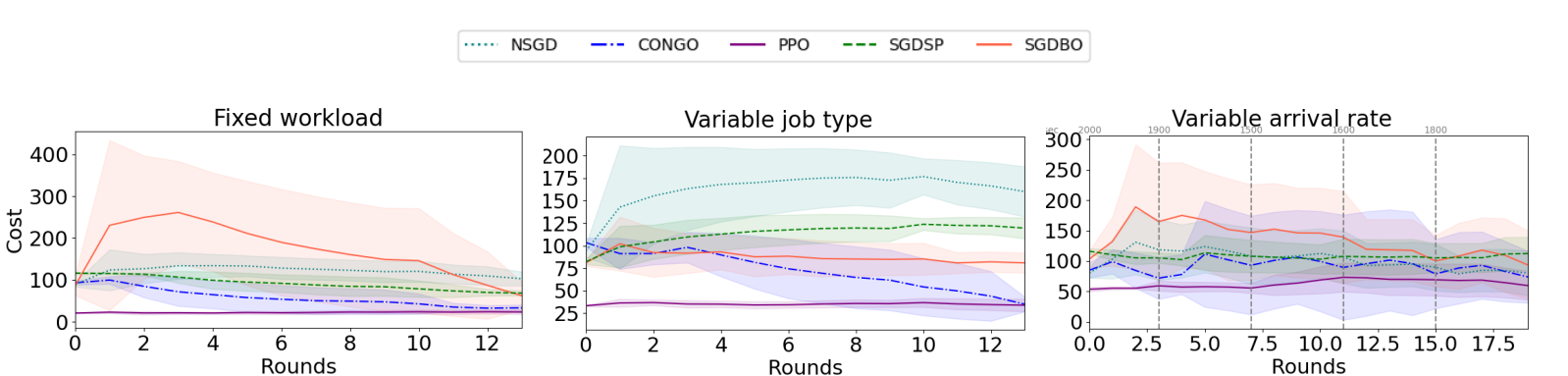
Figure 4: Comparison of algorithms in Jackson network simulations.

Figure 5: Comparison of algorithms for a real-world microservices benchmark application.

7.2 Real-world microservice benchmark deployment

Methodology: In this study, we test CONGO’s ability to converge to an efficient resource allocation when autoscaling on a real-world benchmark. We utilize the SocialNetwork application from the DeathStarBench suite [11]. This application represents a small-scale social media platform with various requests such as ‘compose-post’, ‘read-user-timeline’, and ‘read-home-timeline’. As with the experiments in Section 7.1, three scenarios are considered: (i) fixed workload, (ii) fixed arrival rate with variable job types, and (iii) variable arrival rate with fixed job types. Also similar to those experiments, we use a combination of the end-to-end latency and a cost associated with CPU allocations as the overall cost function. Concretely, if we let $\bar{L}(\cdot,\cdot)$ denote the sample mean of the end-to-end latency as alluded to in Section 3, the cost is calculated as

$$f_{t}(x_{t})=\psi\bar{L}(\lambda_{t},x_{t})+w\sum_{i=1}^{d}[x_{t}]_{i}$$

Note that for the purposes of minimizing the cost function, the introduction of the latency weight $\psi$ has the same effect on the optimal solution as rescaling $w$ by its inverse. In these experiments, we set $\psi=0.001$ and $w=0.1$ which is the inverse of the number of containers involved in the autoscaling process.

Baselines: These experiments compare CONGO against three gradient-descent baselines and one pretrained RL method. We use the NSGD, SGDBO and SGDSP baselines as described in Section 7.1 and PPO as a representative pretrained RL method. We note that pretrained models are a part of several existing autoscaling methods (see Appendix A) but they are usually cumbersome or impractical since they require frequent re-training to adapt to changes in the microservice application. For each experiment, we averaged over four different runs for each algorithm.

Results: As seen in Figure 5, CONGO never performs significantly worse than any of the gradient descent baselines. The superiority of CONGO is most evident in cases where the arrival rate is not changing; in cases where the arrival rate changes, all of the gradient descent-based algorithms suffer from oscillations just like in the simulated system, and this slows the convergence of CONGO. Importantly, CONGO is the only one of the gradient descent baselines to perform competitively in both the variable job type and the variable arrival rate scenarios. Furthermore, CONGO is able to achieve performance rivaling PPO in under 12 rounds with a fixed arrival rate and 15 rounds with a variable arrival rate.

8 Conclusion and limitations

We analyzed and empirically validated the viability of CONGO, an algorithm for OCO when the gradient of the objective function is known to be sparse. We showed in our online setting that with a sufficient number of samples that is largely independent of the problem dimension, we can guarantee $\mathcal{O}\left(s\sqrt{\log(d/s)}\sqrt{T\log(T+1)}\right)$ regret. Theoretically, we characterized the trade-off between reduced sampling and reduced regret. Our experiments demonstrated CONGO’s superiority over general gradient descent algorithms in highly sparse problems and its robustness in approximately sparse cases. We conclude that CONGO can reduce operating costs and improve performance when applied to the management of microservice and other sparse applications.

Limitations: The assumption of exactly sparse gradients in our theoretical analysis may not hold in complex systems, but our empirical results show that near-sparsity suffices for CONGO’s benefits. Empirically we have shown that our algorithm is robust to sample limitations, with $k$ values independent of $T$ still providing competitive results, suggesting that assumptions on $k$ in Theorem 1 can be largely ignored in practice. Also note that the assumption of stability (i.e., job arrival rates do not exceed service rates for prolonged periods) plays a role in the empirical performance of CONGO. Measures to ensure stability are detailed in Appendix C. Finally, solving the $l1$-minimization problem in CONGO can be computationally expensive for high-dimensional problems, resulting in a computational overhead absent in other gradient descent algorithms.

Appendix A Related works

Zeroth-Order Online Convex Optimization: Online Convex Optimization (OCO) is a game in which an online player iteratively makes decisions drawn from a convex set. Upon committing to a decision, the player incurs a loss, which is a possibly advesarially chosen convex function of the possible decisions and is unknown beforehand [12]. In the setting of online convex optimization, there are different levels of information that a learning algorithm may have access to. The first is full information, where the full objective function chosen by the adversary is revealed after the corresponding cost is incurred. If the objective function is also smooth, then regret which scales as $\sqrt{T}$ is achievable by simply running a gradient descent algorithm on the gradients of the revealed functions. Another level of information is bandit information [7; 23], where only the loss is revealed; in this case it is common to rely on zeroth-order methods for gradient estimation. However, stochastic single-point gradient estimators are known to have high variance, and algorithms like the one in [23] rely upon the constraint set having an efficiently computable self-concordant barrier. An intermediate setting between these two extremes allows the algorithm to collect a limited number of samples from the objective function after incurring the loss, which opens up more options for zeroth-order gradient estimation procedures. A general oracle framework for zeroth-order gradient estimation procedures using one or more samples in the OCO context is developed in [13].

Simultaneous Perturbation Stochastic Approximation: The most basic form of SPSA, due to [24], is a method for computing an estimate of $\nabla f(x)$ using only zeroth-order information with only two evaluations of the objective function regardless of the dimension of $x$. Naively, one may compute an approximate measurement of the gradient at $x$ along one dimension as:

$$\frac{\partial f(x)}{\partial x_{i}}\approx\frac{f(x+\delta e_{i})-f(x)}{\delta}.$$ (5)

Where $e_{i}$ is the unit vector in direction $i$, and $\delta$ is the smoothing parameter which controls the bias. However, for a high-dimensional problem this requires at least $d$ measurements in addition to $f(x)$ to estimate the full gradient which might be infeasible due to the time or effort required to take a measurement. The alternative provided by SPSA is as follows: First, generate a sequence of $d$ i.i.d. Rademacher random variables, $\{\Delta_{j}\}_{j=1}^{d}$. Next, generate, a perturbation vector $\Delta:=\sum_{j=1}^{d}e_{j}\Delta_{j}$. Finally, we may compute our gradient estimate as follows:

$$\frac{f(x+\delta\Delta)-f(x)}{\delta\Delta_{j}}\approx\frac{\partial f(x)}{\partial x_{i}}+\sum_{i\neq j}\frac{\partial f(x)}{\partial x_{i}}\frac{\Delta_{i}}{\Delta_{j}}$$

When the expectation is taken over the randomness in $\Delta$, the terms in the summation are eliminated and hence this method gives an approximately unbiased estimate of $\nabla f(x)$ for appropriately small $\delta$. The variance in the estimate can be reduced by repeating the process for different random draws of $\Delta$ and averaging over the results. The SPSA method provides a way to handle high-dimensional problems when the number of available measurements is limited, but it cannot exploit the sparsity of $\nabla f(x)$. This left open the opportunity for improvement of the algorithm using compressive sensing.

Compressive Sensing: Results in compressive sensing [10; 6] state that given measurements of the form $\textbf{{{A}}}x+\eta$ where A is an $m\times d$ matrix with the restricted isometry property with $m$ sufficiently large (called the measurement matrix) and $\eta$ is bounded measurement noise, an approximation $\hat{x}$ can be obtained as the result of an $l1$-minimization problem such that $||\hat{x}-x||_{2}$ is bounded by a quantity proportional to $||\eta||_{2}$. The observation made in [3] that measurements of the form $y=\textbf{{{A}}}\nabla f(x)+\eta$ can be obtained through a method similar to SPSA led to the creation of a simultaneous perturbation gradient estimation algorithm that can indeed exploit the sparsity of $\nabla f(x)$. In particular, [3] showed that if the perturbation vector is ${\textbf{{{A}}}}^{T}\Delta$ where A is the aforementioned measurement matrix and $\Delta$ is a vector of $m$ Rademacher random variables, then the SPSA procedure outputs a vector of dimension $m$ which is suitable for performing sparse recovery.

Microservice Autoscaling: Prior approaches have tried to use several variants of learned models as controllers for the task of allocating resources to microservices. At a high-level, all prior works either rely on heavy complex training regimes, which can be infeasible in practice or make simplifying assumptions as they do not exploit the sparsity in gradients. We now discuss at length, these techniques.

Many prior works [21; 29; 19] rely on complex and heavy offline training mechanisms. This is especially challenging in the microservice setting where frequent re-training might be necessary because applications are regularly updated leading to changes in microservice behavior and even application graphs [14].

FIRM [21] first uses an SVM model to identify the critical bottlenecked service, and then uses an offline-trained DDPG-based model to change the resources for the critical service. A key drawback of this technique is that training FIRM requires anomalies to be injected by artificially inducing resource bottlenecks in the system - which can be either impossible or too expensive in many cases. Injecting resource constraints might be infeasible if the application is run on a third-party cloud provider. On the other hand, it can be expensive if the application undergoes frequent changes/updates.

Sinan [29] predicts if a given resource allocation set for a microservice application can lead to latency violations. Using the predictions, it then relies on a heuristic to choose the next control action. Sinan has two drawbacks. First, training the latency violation predictor requires extensive data on various resource allocation and workload combinations, which is again impractical. Second, the heuristic to change resource allocations might not be general enough for all applications.

Erms [19] approximates the latency-throughput curve for each microservice as a piecewise linear function and employs techniques to prioritize latency-critical services at shared microservices. The assumption of piecewise linear function can be too simplistic for most microservices. Especially, at the inflection points, when a small change in the request rate causes high changes in the latencies, even small error in the piecewise linear estimation can lead to drastically bad performance.

Autothrottle [28] uses an online RL mechanism using contextual bandits and thus, alleviates the problem of offline training to a great extent. However, because Autothrottle does not exploit the sparsity in gradients of microservices, it is forced to make a simplifying assumption by clustering all services into just two clusters, leading to the same action for all services in the same class. This would imply that even if one microservice is the bottleneck, in expectation, it could lead to more resources being allocated for roughly half of all the services!

Erlang [22] is another such online RL-based system for microservice autoscaling, that uses a multi-armed bandit algorithm to choose the right resource allocation, given a congested microservice. However, Erlang relies on a simple heuristic to choose the congested microservice in the first place. The heuristic is to just use the service which has the highest change in CPU utilization. This heuristic may not hold in many cases, for example, when the CPU utilization of a microservice may be high because it is continuously polling on a downstream microservice [11].

Appendix B Proofs

B.1 Proof of Lemma 2

Proof.

First, we invoke Lemma 1 which states that $||\tilde{\nabla}f(x)-\nabla f(x)||_{2}<\frac{2\gamma}{\tau}$ with probability at least $1-\epsilon m$. As noted in Section 4, this holds even with the additional constraint on $||z||_{2}$. But because of this additional constraint, even when the result does not hold we have $||z||_{2}\leq L_{f}+\frac{2\gamma}{\tau}$, implying that

$$||\tilde{\nabla}f(x)-\nabla f(x)||_{2}\leq\frac{2\gamma}{\tau}+L_{f}+||\nabla f(x)||_{2}\leq\frac{2\gamma}{\tau}+2L_{f}$$

Let $E$ denote the event $||\tilde{\nabla}f(x)-\nabla f(x)||_{2}\leq\frac{2\gamma}{\tau}$ and $\bar{E}$ its complement. By the law of total expectation,

$$\displaystyle\begin{array}[]{r@{\ }c@{\ }l@{\ }l}\mathbb{E}\left[\left\lVert\tilde{\nabla}f(x)-\nabla f(x)\right\rVert_{2}^{2}\right]&=&\mathbb{E}\left[\left\lVert\tilde{\nabla}f(x)-\nabla f(x)\right\rVert_{2}^{2}\Bigm{|}E\right]\mathbb{P}\left(E\right)\\ &&+\mathbb{E}\left[\left\lVert\tilde{\nabla}f(x)-\nabla f(x)\right\rVert_{2}^{2}\Bigm{|}\bar{E}\right]\mathbb{P}\left(\bar{E}\right)\\ &\leq&\left(\frac{2\gamma}{\tau}\right)^{2}+\left(\frac{2\gamma}{\tau}+2L_{f}\right)^{2}\epsilon m\\ \end{array}$$

where we use the bound $\mathbb{P}\left(E\right)\leq 1$. The constraints given in Lemma 1 require that

$$m\geq 2s\left(\sqrt{\log\left(\frac{ed}{s}\right)}+\sqrt{\frac{\log(\epsilon^{-1})}{s}}+\frac{\tau}{\sqrt{s}}\right)$$

Furthermore, $\gamma>2mK\delta$ and

$$\epsilon=2\exp\left(-\frac{\gamma^{2}k}{2m^{2}(m-1)G^{2}}\right)<<\frac{1}{m}$$ (6)

where $K\geq||\nabla^{2}f_{t}||_{2}||\textbf{{{A}}}||_{2}$ and $G\geq\sup_{i}|\langle\nabla f(x),a_{i}\rangle|$, with $a_{i}$ being the $i$th row of A (note that these must be bounds which hold for all $t=1,2,\cdots T$). The conditions given in the statement of Lemma 2 are based on these constraints. Note that while [3] does not provide a fixed bound on either of these quantities, since the entries of A come from a standard normal distribution one can find constant bounds large enough to hold with arbitrarily high probability. ∎

B.2 Proof of Theorem 1

In addition to Lemma 2, the proof of Theorem 1 requires the following lemma from [20] expressed in our notation below.

Lemma 3 (Lemma 2.1 of [20]).

Let $V_{\omega}(\cdot,\cdot)$ be the Bregman Distance w.r.t. the $\alpha$-strongly convex distance generating function $\omega$, and let $P_{x}(\cdot)$ be the proximal mapping associated with $\omega$. Then for every $u\in\mathcal{K}$, $x\in\mathcal{K}^{o}$, and $y\in\mathbb{R}^{d}$, one has

$$V_{\omega}(P_{x}(y),u)\leq V_{\omega}(x,u)+\langle y,u-x\rangle+\frac{||y||^{2}_{*}}{2\alpha}$$

Using $x=x_{t}$ and $y=\eta_{t}\tilde{\nabla}f_{t}(x_{t})$, we get

$$\eta_{t}\langle x_{t}-u,\tilde{\nabla}f_{t}(x_{t})\rangle\leq V_{\omega}(x_{t},u)-V_{\omega}(x_{t+1},u)+\frac{\eta_{t}^{2}}{2\alpha}||\tilde{\nabla}f_{t}(x_{t})||^{2}_{*}$$

This result applies generally to mirror descent algorithms, but since projected gradient descent can be viewed as a special case of this in the Euclidean setting, we simplify it to (7) (This form appears in equation 2.6 of [20], where the expectation is taken over all of the terms).

$$\langle\tilde{\nabla}f_{t}(x_{t}),x_{t}-u\rangle\leq\frac{1}{\eta_{t}}\left(\frac{1}{2}||u-x_{t}||^{2}_{2}-\frac{1}{2}||u-x_{t+1}||^{2}_{2}\right)+\frac{\eta_{t}}{2}||\tilde{\nabla}f_{t}(x_{t})||^{2}_{2}$$ (7)

Proof.

Informed by the approach in Section 7.2 of [13], we seek to show that on each round the regret of our algorithm compared to any arbitrary point, which includes $\min_{x^{\star}}\sum_{t=0}^{T-1}f_{t}(x^{\star})$, is sufficiently small. We begin by applying the convexity of $f_{t}$:

$$\displaystyle\begin{array}[]{r@{\ }c@{\ }l@{\ }l}\mathbb{E}\left[\sum_{t=1}^{T}f_{t}(x_{t})-\sum_{t=1}^{T}f_{t}(x)\right]&\leq&\mathbb{E}\left[\sum_{t=1}^{T}\langle\nabla f_{t}(x_{t}),x_{t}-x\rangle\right]\\ &=&\mathbb{E}\left[\sum_{t=1}^{T}\langle\tilde{\nabla}f_{t}(x_{t}),x_{t}-x\rangle+\sum_{t=1}^{T}\langle\nabla f_{t}(x_{t})-\tilde{\nabla}f_{t}(x_{t}),x_{t}-x\rangle\right]\\ &\leq&\mathbb{E}\left[\sum_{t=1}^{T}\langle\tilde{\nabla}f_{t}(x_{t}),x_{t}-x\rangle\right]+\sum_{t=1}^{T}\mathbb{E}\left[\left\lVert\nabla f_{t}(x_{t})-\tilde{\nabla}f_{t}(x_{t})\right\rVert_{2}||x_{t}-x||_{2}\right]\\ &\leq&\mathbb{E}\left[\sum_{t=1}^{T}\langle\tilde{\nabla}f_{t}(x_{t}),x_{t}-x\rangle\right]+\sum_{t=1}^{T}\mathbb{E}\left[2R\left\lVert\nabla f_{t}(x_{t})-\tilde{\nabla}f_{t}(x_{t})\right\rVert_{2}\right]\\ &\leq&\mathbb{E}\left[\sum_{t=1}^{T}\langle\tilde{\nabla}f_{t}(x_{t}),x_{t}-x\rangle\right]+2RT\sqrt{\left(\frac{2\gamma}{\tau}\right)^{2}+\left(\frac{2\gamma}{\tau}+2L_{f}\right)^{2}\epsilon m}\\ \end{array}$$

Focusing on the remaining term, we apply Lemma 3 in the form given by (7), where we let $u=x$. Thus, by telescoping,

$$\displaystyle\begin{array}[]{r@{\ }c@{\ }l@{\ }l}\mathbb{E}\left[\sum_{t=1}^{T}\langle\tilde{\nabla}f_{t}(x_{t}),x_{t}-x\rangle\right]&\leq&\mathbb{E}\left[\sum_{t=1}^{T}\frac{1}{\eta_{t}}\left(\frac{1}{2}||x-x_{t}||^{2}_{2}-\frac{1}{2}||x-x_{t+1}||^{2}_{2}\right)+\eta_{t}\mathbb{E}\left[\frac{||\tilde{\nabla}f_{t}(x_{t})||^{2}_{2}}{2}\right]\right]\\ &\leq&\frac{D}{\eta_{T-1}}+\mathbb{E}\left[\sum_{t=1}^{T}\eta_{t}\frac{||\tilde{\nabla}f_{t}(x_{t})||^{2}_{2}}{2}\right]\end{array}$$

where $D=\underset{x,y\in\mathcal{K}}{\sup}\frac{1}{2}||x-y||^{2}_{2}$. Now, due to the constraints on the $l1$-minimization problem in Algorithm 1 we know that $||\tilde{\nabla}f_{t}(x_{t})||_{2}\leq\frac{2\gamma}{\tau}+L_{f}$, and hence

$$\mathbb{E}\left[\sum_{t=1}^{T}\langle\tilde{\nabla}f_{t}(x_{t}),x_{t}-x\rangle\right]\leq\frac{D}{\eta_{n-1}}+\sum_{t=1}^{T}\eta_{t}\frac{R(\frac{2\gamma}{\tau}+L_{f})^{2}}{2}$$

Putting things together, we have

$$\displaystyle\begin{array}[]{r@{\ }c@{\ }l@{\ }l}\mathbb{E}\left[\sum_{t=1}^{T}f_{t}(Y_{t})\right]-\sum_{t=1}^{T}f_{t}(x)&\leq&\frac{D}{\eta_{n-1}}+\sum_{t=1}^{T}\eta_{t}\frac{R(\frac{2\gamma}{\tau}+L_{f})^{2}}{2}\\ &+&2RT\sqrt{\left(\frac{2\gamma}{\tau}\right)^{2}+\left(\frac{2\gamma}{\tau}+2L_{f}\right)^{2}\epsilon m}\end{array}$$ (10)

The terms which will have the greatest impact on the order of the regret bound are the last two, so we focus on them first. Noting that $\epsilon m>0$, we have the following inequality:

$$\displaystyle\begin{array}[]{r@{\ }c@{\ }l@{\ }l}2RT\sqrt{\left(\frac{2\gamma}{\tau}\right)^{2}+\left(\frac{2\gamma}{\tau}+2L_{f}\right)^{2}\epsilon m}&\leq&\frac{4RT\gamma}{\tau}+4RT\left(\frac{\gamma}{\tau}+L_{f}\right)\sqrt{\epsilon m}\\ &\leq&\frac{4RT\gamma}{\tau}(1+\sqrt{\epsilon m})+4RTL_{f}\sqrt{\epsilon m}\end{array}$$ (13)

By Lemma 2, we need $\gamma>2mK\delta$; to achieve this, we set $\gamma=(2mK+1)\delta$. For the first term, we can control the scaling with respect to $T$ by choosing $\delta$ to decrease with $T$; in particular, we can set $\delta=\frac{1}{\sqrt{T}}$ to achieve $\mathcal{O}\left(\sqrt{T}\right)$ scaling (ignoring for now the contribution of $m$ and $\frac{1}{\tau}$). For the second term, to maintain the same scaling we must have $\epsilon=\mathcal{O}\left(\frac{1}{T}\right)$. From this constraint, we can determine a valid choice of $k$ as follows:

$$\displaystyle\begin{array}[]{r@{\ }c@{\ }l@{\ }l}&&\epsilon=\frac{1}{T}\\ &\implies&2\exp\left\{-\frac{(2mK+1)^{2}\delta^{2}k}{2m^{2}(m-1)G^{2}}\right\}=\frac{1}{T}\\ &\implies&\frac{(2mK+1)^{2}k}{2m^{2}(m-1)G^{2}}=T\log(2T)\\ &\implies&k=\frac{2m^{2}(m-1)G^{2}}{(2mK+1)^{2}}T\log(2T)\end{array}$$

Note that $G$ is defined in Lemma 1. Since $k$ must be an integer, we take the ceil of this quantity.

For the first two terms of the overall bound, we have

$$\displaystyle\begin{array}[]{r@{\ }c@{\ }l@{\ }l}\frac{D}{\eta_{T-1}}+\sum_{t=1}^{T}\eta_{t}\frac{R(\frac{2t}{\tau}+L_{f})^{2}}{2}&=&\frac{D}{\eta_{T-1}}+\sum_{t=1}^{T}\eta_{t}\left(2R\left(\frac{(2mK+1)\delta}{\tau}\right)^{2}+2RL_{f}\frac{(2mK+1)\delta}{\tau}+RL_{f}^{2}\right)\\ &=&\frac{D}{\eta_{T-1}}+\sum_{t=1}^{T}\eta_{t}\left(\frac{2R}{T}\left(\frac{(2mK+1)}{\tau}\right)^{2}+\frac{2RL_{f}(2mK+1)}{\tau\sqrt{T}}+RL_{f}^{2}\right)\end{array}$$

Due to the $RL_{f}^{2}$ term inside the parentheses, the second term will scale as $\mathcal{O}\left(\sum_{t=1}^{T}\eta_{t}\right)$ while the first term will scale as $\frac{1}{\eta_{T-1}}$ We balance this by choosing $\eta_{t}=\frac{1}{\sqrt{T}}$, such that the overall expression scales as $\mathcal{O}\left(\sqrt{T}\right)$.

It remains now to choose $m$ and $\tau$. The main constraint is

$$\frac{m^{2}}{m+1} \geq 2s\left(\sqrt{\log\left(\frac{ed}{s}\right)}+\sqrt{\frac{\log(\epsilon^{-1})}{s}}+\frac{\tau}{\sqrt{s}}\right)$$

or simply

$$m \geq 2s\left(\sqrt{\log\left(\frac{ed}{s}\right)}+\sqrt{\frac{\log(\epsilon^{-1})}{s}}+\frac{\tau}{\sqrt{s}}\right)$$

where $\log(\epsilon^{-1})=\log(T)$. Notice that $\tau$ only appears in the denominator of terms which have $\gamma$ (and hence a factor of $m$) in the numerator, so we want to optimize the ratio $\frac{m}{\tau}$. If we choose $\tau=\sqrt{\log(T)}$ then we get $m=\mathcal{O}\left(\log(T)\right)$ and $\frac{m}{\tau}=\mathcal{O}\left(\sqrt{\log(T)}\right)$; but we want to avoid a situation where $\tau=\sqrt{\log(1)}=0$ so we choose $\tau=\sqrt{\log(T+1)}$ instead. We can still combine the last two terms in $m$ if we let

$$\displaystyle\begin{array}[]{r@{\ }c@{\ }l@{\ }l}m&=&\left\lceil 2s\left(\sqrt{\log\left(\frac{ed}{s}\right)}+\sqrt{\frac{\log(T+1)}{s}}+\frac{\tau}{\sqrt{s}}\right)\right\rceil\\ &=&\left\lceil 2s\left(\sqrt{\log\left(\frac{ed}{s}\right)}+\sqrt{\frac{2\log(T+1)}{s}}\right)\right\rceil\end{array}$$

The dominant terms scale as $\mathcal{O}\left(s\sqrt{\log\left(\frac{ed}{s}\right)T}\right)$ and $\mathcal{O}\left(\sqrt{T\log(T+1)}\right)$, which we combine to get a $\mathcal{O}\left(s\sqrt{\log(\frac{d}{s})}\sqrt{T\log(T+1)}\right)$ regret scaling. Furthermore, we have $k=\mathcal{O}\left(T\log(2T)\log(T+1)\right)$. Written out in full, the regret bound is

$$\displaystyle\begin{array}[]{r@{\ }c@{\ }l@{\ }l}\mathbb{E}\left[\sum_{t=1}^{T}f_{t}(x_{t})\right]-\sum_{t=1}^{T}f_{t}(x)&\leq&D\sqrt{T}+\frac{2R(2Km+1)^{2}}{\sqrt{T}(\log(T+1))}+\frac{2RL_{f}(2Km+1)}{\sqrt{\log(T+1)}}\\ &+&RL_{f}^{2}\sqrt{T}+\frac{4R(2Km+1)\sqrt{T}}{\sqrt{\log(T+1)}}\left(1+\sqrt{\frac{m}{T}}\right)\\ &+&4RL_{f}\sqrt{mT}\end{array}$$

∎

B.3 Proof of Corollary 1

Proof.

Fix $p>0$ and set $\delta=T^{-\frac{1}{2q}+p}$ in the algorithm. Note that our choice of $\gamma=2m^{\frac{3}{2}}K\delta$ satisfies $\gamma>2mK\delta$ assuming that $m>1$. Given this choice of $\gamma$, the constraint on $\epsilon$ from (6) becomes

$$\displaystyle\begin{array}[]{r@{\ }c@{\ }l@{\ }l}\epsilon&=&2\exp\left(-\frac{4m^{3}K^{2}\delta^{2}k}{2m^{2}(m-1)G^{2}}\right)\\ &\leq&2\exp\left(-\frac{4m^{3}K^{2}}{2m^{3}G^{2}}T^{-\frac{2}{2q}+2p}T^{\frac{1}{q}}\right)\\ &=&2\exp\left(-2\frac{K^{2}}{G^{2}}T^{-\frac{1}{q}+2p}T^{\frac{1}{q}}\right)\\ &=&2\exp\left(-2\frac{K^{2}}{G^{2}}T^{2p}\right)\end{array}$$

Since $p>0$, we have exponential decay for $\epsilon$ as opposed to the $\mathcal{O}\left(\frac{1}{T}\right)$ scaling we have in Theorem 1. Thus, the terms in the regret bound that include $\epsilon$ will not be the dominant terms in the asymptotic regret (for small $T$, of course, they may be dominant). Now, if we choose $m$ the same way we did in the proof of Theorem 1, we get

$$m=\Theta\left(\sqrt{s\log(\epsilon^{-1}}\right)=\Theta\left(\sqrt{sT^{2p}}\right)=\Theta\left(\sqrt{s}T^{p}\right)$$

Similar to the proof of Theorem 1, we set $\tau=\sqrt{\log(\epsilon^{-1})}=\Theta\left(T^{p}\right)$ so that the scaling of $m$ remains the same. To analyze the regret under these new parameter choices, we follow the same steps as in the proof of Theorem 1 up to (10). At that point, after plugging in $\eta_{t}=\frac{1}{\sqrt{T}}$, we get the following asymptotic bound:

$$\displaystyle\begin{array}[]{r@{\ }c@{\ }l@{\ }l}\mathbb{E}\left[\sum_{t=1}^{T}f_{t}(Y_{t})\right]-\sum_{t=1}^{T}f_{t}(x)=&&\mathcal{O}\left(\sqrt{T}\right)+\mathcal{O}\left(\left(\frac{\gamma}{\tau}\right)^{2}\sqrt{T}\right)+\mathcal{O}\left(\frac{\gamma}{\tau}\sqrt{T}\right)+\mathcal{O}\left(\frac{\gamma}{\tau}T\right)\\ +&&\mathcal{O}\left(\frac{\gamma\sqrt{\epsilon m}}{\tau}T\right)+\mathcal{O}\left(\sqrt{\epsilon m}T\right)\end{array}$$

Based on the new parameter choices, the dominant term here is the one which scales as $\mathcal{O}\left(\frac{\gamma}{\tau}T\right)$. Note that

$$\frac{\gamma}{\tau}=\mathcal{O}\left(\frac{m^{\frac{3}{2}}\delta}{\tau}\right)=\mathcal{O}\left(s^{\frac{3}{4}}T^{\frac{p}{2}}T^{-\frac{1}{2q}+p}\right)=\mathcal{O}\left(s^{\frac{3}{4}}T^{\frac{3p}{2}-\frac{1}{2q}}\right)$$

This means that the dominant term scales as

$$\mathcal{O}\left(s^{\frac{3}{4}}T^{\frac{3p}{2}-\frac{1}{2q}+1}\right)=\mathcal{O}\left(s^{\frac{3}{4}}T^{\frac{2q-1}{2q}+\frac{3p}{2}}\right)$$

Since we can let $p$ be arbitrarily close to 0 while keeping the exponential decay of $\epsilon$, we can have an overall regret that is arbitrarily close to $\mathcal{O}\left(T^{\frac{2q-1}{2q}}\right)$. ∎

B.4 Proof of Theorem 2

Proof.

$$\displaystyle\begin{array}[]{r@{\ }c@{\ }l@{\ }l}\mathbb{E}\left[||{\textbf{{{A}}}}^{T}\Delta||_{2}\right]&=&\mathbb{E}\left[\sqrt{{\Delta}^{T}\textbf{{{A}}}{\textbf{{{A}}}}^{T}\Delta}\right]\\ &\leq&\sqrt{\mathbb{E}\left[{\Delta}^{T}\textbf{{{A}}}{\textbf{{{A}}}}^{T}\Delta\right]}\textrm{ }\left(\textrm{By the concavity of $\displaystyle\sqrt{\cdot}$}\right)\\ &=&\sqrt{\mathbb{E}\left[\textrm{trace}\left({\Delta}^{T}\textbf{{{A}}}{\textbf{{{A}}}}^{T}\Delta\right)\right]}\\ &=&\sqrt{\mathbb{E}\left[\textrm{trace}\left(\Delta{\Delta}^{T}\textbf{{{A}}}{\textbf{{{A}}}}^{T}\right)\right]}\\ &=&\sqrt{\textrm{trace}\left(\mathbb{E}\left[\Delta{\Delta}^{T}\right]\mathbb{E}\left[\textbf{{{A}}}{\textbf{{{A}}}}^{T}\right]\right)}\\ &=&\sqrt{\textrm{trace}\left(\textbf{I}_{m}\mathbb{E}\left[\textbf{{{A}}}{\textbf{{{A}}}}^{T}\right]\right)}\\ &=&\sqrt{\mathbb{E}\left[\textrm{trace}\left(\textbf{{{A}}}{\textbf{{{A}}}}^{T}\right)\right]}\\ &=&\sqrt{\sum_{i=1}^{m}\mathbb{E}\left[\left\lVert a_{i}\right\rVert_{2}^{2}\right]}\\ \end{array}$$

We now invoke Proposition 8.1(b) of [10], which implies that $\mathbb{E}\left[\left\lVert a_{i}\right\rVert_{2}^{2}\right]=d$. The claim follows. ∎

Appendix C Details of experimental setup

C.1 Algorithm implementation details

Besides our algorithm, there are several other algorithms which we use in our experiments for Sections 6 and 7. In this section, we provide implementation details for those algorithms as well as additional details on how we implemented CONGO. Note that the difference between the gradient descent algorithms and the stochastic gradient descent algorithms is that the gradient descent algorithms are applied to the experiments in Section 6 where exact function evaluations are available, while the stochastic gradient descent algorithms are applied to the experiments in Section 7 where one must average over noisy samples instead. In the case of CONGO, we use the same name for both to avoid confusion although there are differences in the implementation. Finally, note that there are additional hyperparameters for each of the algorithms used on the real system, which are defined in Table 10.

Gradient Descent: Since we are able to calculate the true gradient of the quadratic functions considered in Section 6, we implement a standard projected gradient descent algorithm with a fixed learning rate.

Naive Stochastic Gradient Descent: This zeroth-order algorithm applies a perturbation to each dimension of $x_{t}$ one at a time and uses the finite difference approximation (as in (5)) to estimate the gradient on a per-dimension basis. This means that the equivalent value of $k$ for this algorithm is always $d$. Furthermore, we normalize the estimated gradient vector and allow a predefined learning rate to determine how much the control moves on each iteration. Our early testing showed that for our target application of autoscaling, normalization is very helpful for stability.

Gradient Descent/Stochastic Gradient Descent with Simultaneous Perturbations: This is an implementation of Spall’s SPSA (see Appendix A for details). Since this algorithm is able to estimate the full gradient after just one measurement like CONGO, we average over $k$ perturbed measurements. For GDSP we apply the gradient estimate to the update step directly, while for SGDSP we normalize it as with NSGD. In the simulation experiments of Section 7.1, we let $k=d$ for SGDSP and CONGO to maintain a fair comparison with NSGD.

Stochastic Gradient Descent with Bayesian Optimization: SGDBO uses the same gradient estimation procedure as NSGD, but eliminates the learning rate hyperparameter altogether by instead solving an intermediate optimization problem on each round that finds the optimum step size. To solve this optimization problem using Bayesian optimization, we use the gp_minimize function from the scikit-optimize Python package, which first randomly selects 10 points along the line at which to evaluate the cost function and then uses an acquisition function based on a Gaussian process model to find good candidates for further exploration, eventually returning the point which achieved the lowest cost. The number of samples used for Bayesian optimizaton is denoted $N_{calls}$; this is not the same as $k$ since the samples are used after the gradient has already been estimated. For each point that the optimizer chooses to query, the simulator runs an environment step and provides the resulting cost back to the optimizer. The complete algorithm for SGDBO is given in Algorithm 2. Here, $x_{max}$ and $x_{min}$ correspond to the upper and lower limits for how much of the resource can be allocated to a microservice (assumed to be uniform across all microservices). $\mathbf{x}_{0}$ gives the initial allocation levels for the microservices, and $\delta,L_{search},N_{calls}$ are the hyperparameters. We note that the direction $\mathbf{v}$ is calculated so that it points opposite the direction of the gradient, hence we move in that direction when we perform the update in line 19. In order for the full SGDBO procedure to be used, it is necessary to take more than $d$ samples, and hence SGDBO has the advantage of more objective function evaluations than the other gradient descent-based algorithms. However, it is highly susceptible to noise since high noise in a function evaluation can make a candidate seem much better than it really is. In our implementation of SGDBO, we specialize to the case where $\mathcal{K}$ is a hypercube centered on the origin such that each dimension of the control point must be in the range $[x_{min},x_{max}]$.

Algorithm 2 Stochastic Gradient Descent with Bayesian Optimization

1:  function SGDBO($x_{max},x_{min},\mathbf{x}_{1},\delta,L_{search},N_{calls}$)

2:  while not converged do

3:     Initialize $\mathbf{v}$ with zeros

4:     $c_{max}\leftarrow L_{search}$

5:     for $i=1\cdots d$ do

6:        if $x_{i,t}+\delta\leq x_{max}$ then

7:           $v_{i}\leftarrow f(\mathbf{x_{t}})-f(\mathbf{x_{t}}+\delta)$

8:        else

9:           $v_{i}\leftarrow f(\mathbf{x_{t}}+\delta)-f(\mathbf{x_{t}})$

10:        end if$\triangleright$ Get gradient estimate along each dimension

11:        if $v_{i}<0$ then

12:           $c_{max}\leftarrow\textrm{min}(c_{max},|x_{i,t}-x_{min}|)$

13:        else

14:           $c_{max}\leftarrow\textrm{min}(c_{max},|x_{i,t}-x_{max}|)$

15:        end if$\triangleright$ Reduce search space to avoid stepping outside of $\mathcal{K}$

16:     end for

17:     $\mathbf{v}\leftarrow\mathbf{v}/||\mathbf{v}||$

18:     $c\leftarrow\textrm{gp\_minimize}(c_{max},N_{calls})$ $\triangleright$ Bayesian optimization

19:     $x_{t+1}\leftarrow x_{t}+c\mathbf{v}$

20:     $t\leftarrow t+1$

21:  end while

22:  end SGDBO

RL Agent Using Proximal Policy Optimization: Proximal Policy Optimization (PPO) is a trust region based policy gradient algorithm that maximizes the following objective function

$$L\left(s,a,\theta_{k},\theta\right)=\min\left(\frac{\pi_{\theta}(a\mid s)}{\pi_{\theta_{k}}(a\mid s)}A^{\pi_{\theta_{k}}(s,a),}\operatorname{clip}\left(\frac{\pi_{\theta}(a\mid s)}{\pi_{\theta_{k}}(a\mid s)},1-\epsilon,1+\epsilon\right)A^{\pi_{\theta_{k}}}(s,a)\right)$$ (14)

This objective function ensures that the policy updates are not too drastic. Specifically, the gradient of the objective goes to zero if the ratio of the new policy probability to the old policy probability for any given state-action pair deviates more than $\epsilon$ away from 1. The PPO agent is trained on the DeathStarBenchmark Social Media environment (we do not use it in the Jackson network simulations) for 30 iterations to learn the impact of different CPU allocations on system performance. It is then tested for an additional 30 iterations to evaluate its effectiveness, which is what we compare to the other algorithms. PPO was chosen as a baseline to demonstrate the performance of an algorithm with prior system knowledge, unlike gradient descent approaches.

Compressive Online Gradient Optimization: In the simulation experiments of Section 7.1, we let $k=d$ for SGDSP and CONGO to maintain a fair comparison with NSGD. We note that in the implementation of CONGO, there is flexibility in what numerical method to use for finding an approximate solution the $l1$-minimization problem; one option that we have had success with is Chambolle and Pock’s primal-dual algorithm (see [10], Section 15.2), but this algorithm is computationally expensive so for the experiments on the DeathStarBench Social Network Application where actions must be taken in real-time, we instead use an SLSQP non-linear solver.
Sequential Least Squares Quadratic Programming (SLSQP) is an optimization technique that iteratively approximates a nonlinear problem by solving a sequence of quadratic subproblems, each subject to linearized constraints. This method is highly effective for constrained optimization, incorporating both equality and inequality constraints. We use the implementation provided by the scipy optimize Python package.

C.2 Numerical experiments for online optimization of quadratic functions

For all three of the experiments shown in Figure 3, we used $T=100$. Table 1 shows how the hyperparameters for CONGO are set when running the experiments of section 6. Note that the only hyperparameter required for GD is the learning rate, and the only hyperparameters required for GDSP are the learning rate, $\delta$, and $k$; these parameters match the values used for CONGO unless otherwise specified.

Table 1: Hyperparameters for Numerical Experiments

Name	Description	Value
lr	learning rate	0.1
$\delta$	smoothing parameter	0.01
$k$	# SPSA samples to average	varies
$m$	# rows in A	$\lceil s\log(d)\rceil$
$\gamma$	noise bound	$\begin{cases}2m\sqrt{2\log(2d)}||\textbf{{{A}}}||_{2}\delta,&d=50\\ 1,&d=200\end{cases}$

The bound on $\gamma$ when $d=50$ is based on the requirement given in 1, where $\sqrt{2\log(2d)}$ serves as an upper bound for $\nabla^{2}f_{t}$. However, when $d=200$ this bound becomes too loose and as a result $\gamma$ becomes too large to get good results out of gradient estimation procedure (specifically, the tolerance for error becomes so great that we almost always get $\tilde{\nabla}f_{t}(x_{t})=0$). To resolve this, we somewhat arbitrarily set $\gamma=1$ which gives good results.

For performing computations, the main Python packages we use are Numpy and Pytorch (a full list of the packages required is available with the code). To implement the $l1$-minimization step in CONGO, we use our implementation of Chambolle and Pock’s primal-dual algorithm (see [10], Section 15.2). The seeds we used to obtain our results are 0-49 for the first two plots and 0-9 for the third plot. When creating our plots, we plot the average over the trajectories from the different seeds and also plot a shaded area representing $\pm$ one standard deviation away from the mean. The computation of the mean and standard deviation is done using functions provided by Numpy.

C.2.1 Specifications of machine used

The numerical simulations were run on a machine with an Intel core i7 processor and an NVIDIA GeForce RTX 3050 Ti Laptop GPU. We found that each overall experiment did not take much longer than an hour to run when using the GPU; we did not test the runtime on CPU only.

C.3 Simulation experiments for online optimization of jackson networks

The following information concerns Section 7.1. We first provide a description of the layout of the Jackson networks and briefly explain how they are implemented, then describe the simulated workloads used, and finally provide the hyperparameter settings for the algorithms in Tables 6-9. Any additional information needed to setup and reproduce the experiments is provided with the code.

C.3.1 Jackson network layout

Our simulation experiments use two different layouts, one which we call the complex environment and one which we call the large-scale environment. The first contains 15 microservices and the second contains 50 (recall from Section 3 that we treat a microservice as synonymous with a queue/server node in this model). For each layout we define a set of jobs, each of which is defined by an ordered sequence of microservices which that job must be processed by. The length of this sequence varies from 1 to 7. All jobs share a single entry point which we label as “A". While the queueing-tool package comes with all the functionality needed to simulate a generic Jackson network, we found the need to implement a subclass of the Agent class to implement jobs with paths randomly chosen from a fixed set. However, this did not involve modifying the source code of the package.

A visual representation of the complex environment is given in Figure 6. This environment has eight possible job types, named Job1 through Job8. The sequence of microservices that each type must visit is specified in the .yaml configuration files corresponding to the complex environment. The large-scale environment has a simpler structure; there are 10 job types, and after being processed by the entry-point microservice each job moves through a unique sequence of four or five microservices before exiting the system. Hence, in the large-scale environment the job paths only overlap at the entry point.

In the queueing-tool framework, each microservice is represented as a pair of nodes with a queue edge inbetween. When a job leaves a microservice’s queue, it instantaneously moves from the exit node of that microservice to the entry node of the next and is enqueued on the next microservice’s queue. Using the functionality provided by the queueing-tool package, we generate arrivals according to a Poisson process. Each time a job arrival occurs, the new job has a job type assigned to it according to the workload distribution. The service times, and hence the measured latencies, are based on the Jackson network’s simulation time. We advance the simulation time only when the algorithm incurs its cost for the round or takes one of its $k$ samples (thus nothing changes in the simulation while the algorithm is performing computations). When the average latency is measured, we first advance the simulation for 30 seconds to bring it to a steady state and then advance it for another 10 seconds while measuring the end-to-end latencies experienced by all jobs which leave the system during that period. At the end of a round, we use the clear() function provided by queueing-tool to reset the Jackson network to its initial state. We found this necessary because otherwise the Python object simulating the network would accumulate too much logged data which would make obtaining latency for newly processed jobs prohibitively slow. Running the simulation so that it reaches steady state before taking any measurements compensates for this, since the network is allowed to reach approximately the same state that it would have had under the new allocation without the reset.

Protecting against instability: To ensure that any algorithm has valid latency measurements to use when forming a gradient estimate, we monitor whether or not any jobs leave the system during a measurement period and if none do, we assume that the stability of the Jackson network has been violated. Regardless of which algorithm is in use, when this occurs we increase the allocation to every microservice by a small amount called the correction factor and proceed to the next round. This ensures that the algorithm is able to eventually recover from the instability even if it cannot form a gradient estimate. The choice of correction factor depends on the environment; for the complex environment it is 1, and for the large-scale environment it is 0.1.

Besides the workload, there are a few other parameters which determine the environment that the algorithms operate in. These are the initial allocations for the microservices, the range of allowable allocations, and the resource weight (referred to as $w$ in the paper). For all experiments, the resource weight is set to 1 and the range of allowable allocations is the set [1, 60]. The initial allocations vary based on the experiment since in cases where the workload will change, we want the algorithms to have a chance to converge before the change becomes significant, forcing them to adjust. For simplicity, we keep this value uniform for all but the entry microservice (which requires a higher initial allocation to ensure stability in some cases).

Table 2: Initial Allocation by Configuration

Configuration	Init. Alloc. for Entry Microservice	Init. Alloc. for Others
Complex, Fixed Workload	10	10
Complex, Variable Arrival Rate	10	10
Complex, Variable Job Type	10	7
Large-Scale, Fixed Workload	7	7
Large-Scale, Variable Arrival Rate	7	7
Large-Scale, Variable Job Type	10	4

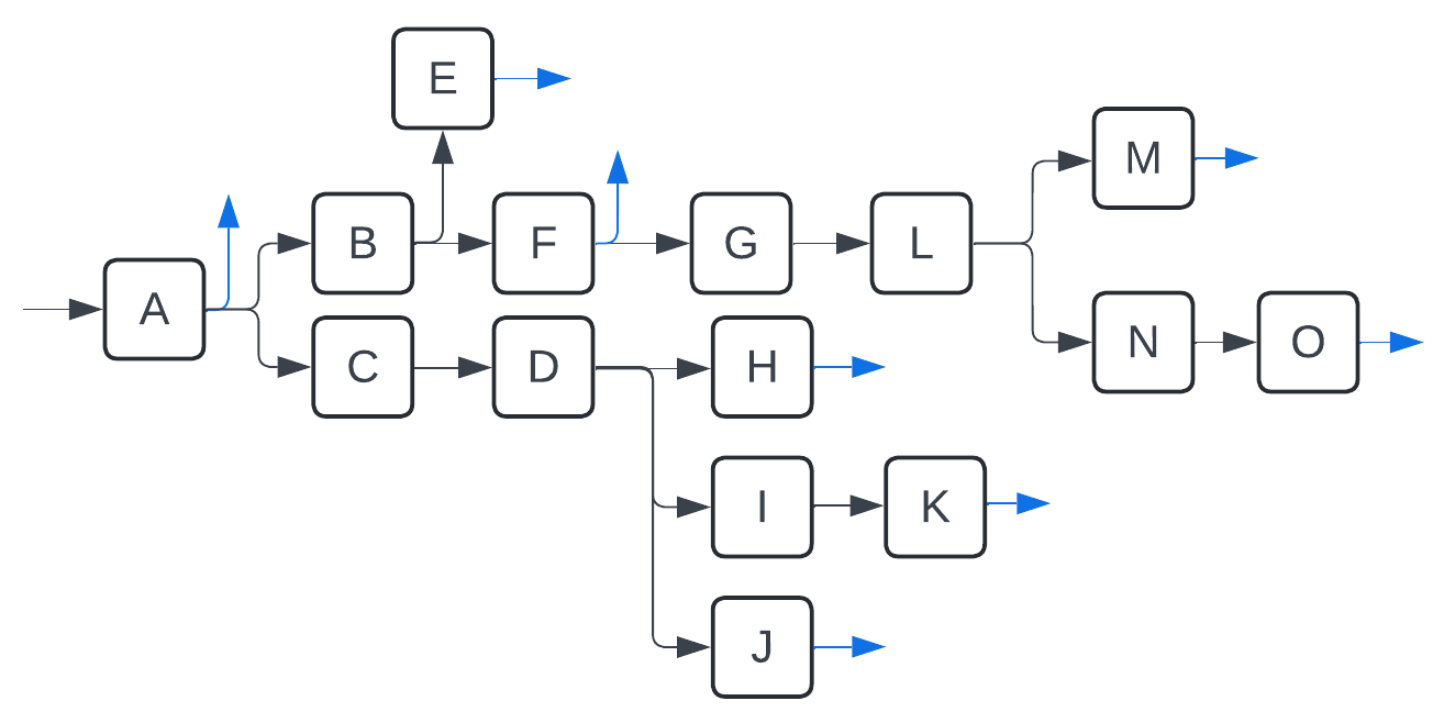
Figure 6: Visual representation of the connections between microservices for the 15-microservice environment. The labeled boxes correspond to microservices, the black arrows correspond to the entry point and the connections between microservices, and the blue arrows correspond to exit points. Each of the 8 possible jobs uses a different exit point.

C.3.2 Description of workloads

The three workload types tested mimic the different workload types used in our experiments on the DeathStarBench Social Network Application. The first type is the fixed workload where both the average arrival rate and the job distribution remain constant for all rounds. The second type is the variable arrival rate workload where the average arrival rate changes periodically while the job distribution remains constant. This workload forces the algorithm to adapt its allocation over time without directly changing the sparsity. The third type is the variable job type workload where the job distribution incrementally switches between two fixed distributions over a certain number of rounds; outside of those rounds, the job distribution is constant. This workload forces the algorithm to adapt to a change in which microservices require resources and hence a change in the sparsity as well. In Tables 3-5, we specify the parameters defining the workload used in each plot of Figure 5.

Table 3: Parameters for Fixed Workloads

Environment	Arrival Rate	Job Distribution
Complex	5/s	Jobs 1,3,4,6,7,8: 2%
		Jobs 2,5: 44%
Large-scale	5/s	Job6: 100%

Table 4: Parameters for Variable Arrival Rate Workloads

Environment	Arrival Rate	Job Distribution
Complex	Rounds 1-25: 5/s	Job6: 100%
	Rounds 26-50: 7/s
	Rounds 51-75: 5/s
	Rounds 76-100: 6/s
Large-scale	Rounds 1-10: 4.5/s	Job2: 100%
	Rounds 11-20: 4.75/s
	Rounds 21-30: 5/s
	Rounds 31-40: 5.25/s
	Rounds 41-50: 5.5/s
	Rounds 51-60: 5.25/s
	Rounds 61-70: 5/s
	Rounds 71-80: 4.75/s
	Rounds 81-90: 4.5/s
	Rounds 91-100: 4.75/s

Table 5: Parameters for Variable Job Type Workloads

Environment	Arrival Rate	Initial Job Distribution	Final Job Distribution	Transition Rounds
Complex	5/s	Job 3: 30%	Job 6: 50%	50-80
		Job 5: 70%	Job 8: 50%
Large-scale	4/s	Job 1: 50%	Job1: 30%	40-90
		Job 3: 50%	Job3: 30%
			Job6: 20%
			Job8: 20%

C.3.3 Hyperparameters

Learning Rate Schedules Since our goal was to show that CONGO produces better gradient estimates than other algorithms, we ensure that NSGD, SGDSP, and CONGO all use the same learning rate schedule so that no algorithm has a clear advantage in that respect (SGDBO is an exception because its search space can extend further than the step size of these algorithms, but this can also make it harder for SGDBO to converge to the optimal value with high accuracy). We use different learning rate schedules for different scenarios since the scenarios have different requirements (e.g. for the large-scale environment we generally need the learning rate to be larger since the gradient estimates are normalized and hence much less change is applied to each microservice for the same learning rate). We list those schedules here:

• Complex environment, fixed workload: Learning rate starts at 1, and is scaled by 0.2 every 25 steps

• Complex environment, variable arrival rate: Learning rate starts at 1, and is reduced to 0.5 after 20 rounds

• Complex environment, variable job type: Learning rate starts at 0.7, and is reduced to 0.35 after 40 rounds

• Large-scale environment, fixed workload: Learning rate is fixed at 1

• Large-scale environment, variable arrival rate: Learning rate is fixed at 1

• Large-scale environment, variable job type: Learning rate starts at 1, and is scaled by 0.5 every 20 steps

The algorithm-specific hyperparameters are specified below

Table 6: NSGD Hyperparameters for Jackson Network Simulation

Hyperparameter	Value
$\delta$ (gradient estimation)	0.02
learning rate	varies - see Learning Rate Schedules

Table 7: SGDSP Hyperparameters for Jackson Network Simulation

Hyperparameter	Value
$\delta$ (gradient estimation)	0.02
learning rate	varies - see Learning Rate Schedules
$k$	matches # of microservices

Table 8: SGDBO Hyperparameters for Jackson Network Simulation

Hyperparameter	Value
$\delta$ (gradient estimation)	0.02
$L_{search}$	10
$N_{calls}$	12

Table 9: CONGO Hyperparameters for Jackson Network Simulation

Hyperparameter	Value
$\delta$ (gradient estimation)	0.02
learning rate	varies - see Learning Rate Schedules
$k$	matches # of microservices
$\gamma$	0.01
$m$	$\begin{cases}6,&\textrm{complex environment}\\ 11,&\textrm{large-scale environment}\end{cases}$

C.3.4 Specifications of machine used

Note that these simulations did not require the use of GPUs.

• Operating System: Ubuntu 22.04.3 LTS (Jammy)

• Kernel Version: 6.5.0-28-generic

• CPU: AMD Ryzen Threadripper 3960X 24-Core Processor

  • Architecture: x86_64

  • Cores: 12

  • Threads: 24

  • Max Frequency: 3.8 GHz

• Memory:

  • Total Memory: 96 GiB

  • Swap: 31 GiB

The runtime for a single trial with one algorithm on this machine varied from 3 to 8 minutes depending on the algorithm for the 15-microservice environment, and from 20 to 40 minutes for the 50-microservice environment.

C.4 DeathStarBench social network application

Overview

The DeathStarBench suite includes a social network application designed to evaluate microservices’ performance. This application simulates real-world social network activities, providing a robust environment for benchmarking.

Testing methodology

The wrk2 tool is utilized to generate workloads for the microservice application. This application consists of multiple containers, each hosting a different microservice. Integrated within these containers are Jaeger clients, which continuously record service-level metrics, specifically latency, in the background. These metrics are periodically sent to the Jaeger Collector.

The collected metrics serve as key performance indicators (KPIs) to assess the system’s performance. The KPIs are then used to calculate the gradient, which informs the adjustments needed for CPU allocations. These adjustments are applied to the system’s containers through Docker commands.

The specific methods for calculating the gradient and implementing CPU allocation modifications are algorithm-dependent. This adaptive approach ensures optimal resource allocation, thereby enhancing the overall efficiency and performance of the microservice application. Figure 7 illustrates how algorithms interact with the social network application in our experiments.

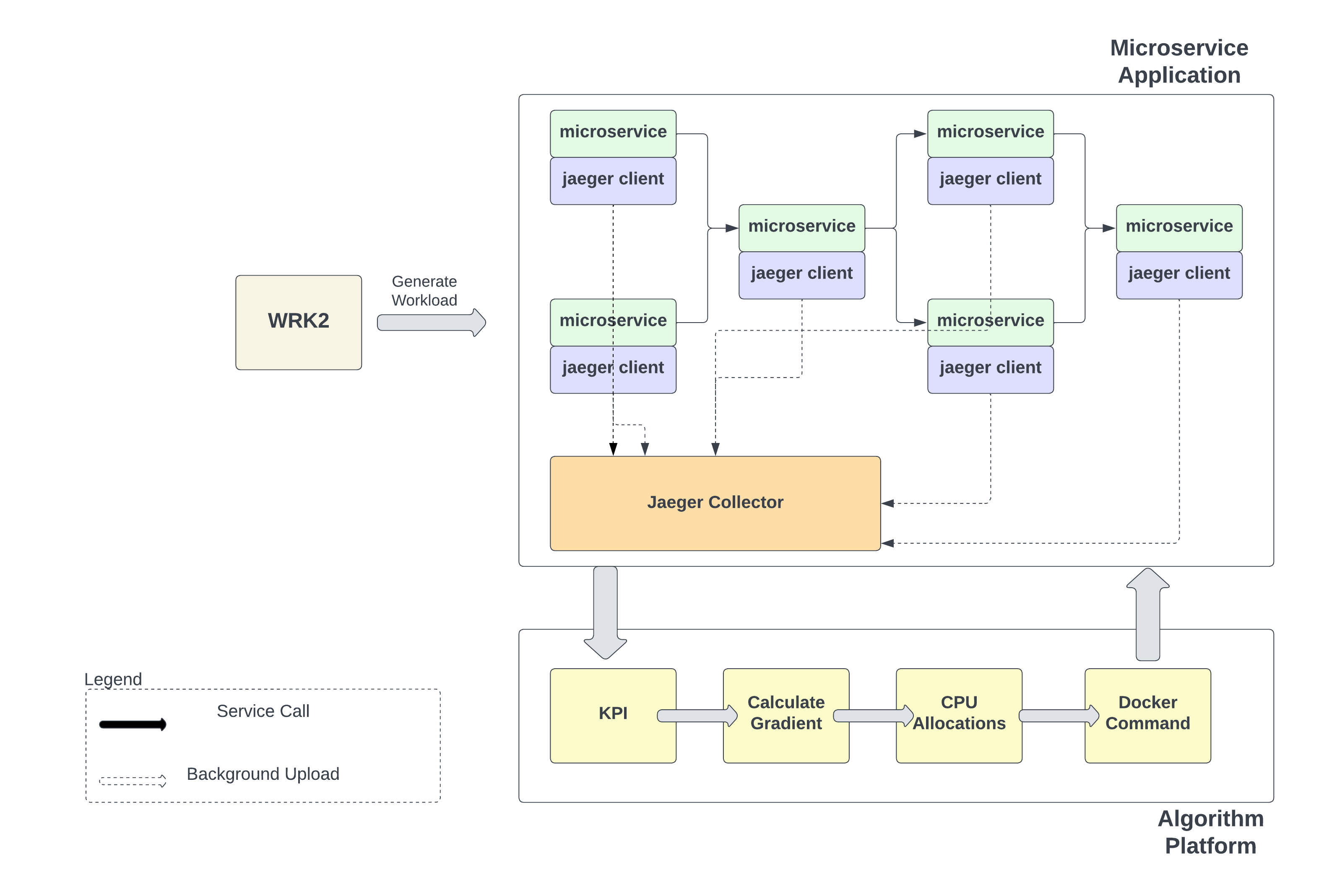
Figure 7: A visual representation of the application of algorithms within a microservice architecture, demonstrating how CPU allocations are adjusted to achieve optimal performance thresholds.

Workloads: We used the WRK2 tool to generate workloads for our experiments. We run the workload for a duration of 2 hours, with 4 client connections. We executed the benchmark against the following workloads:

• Fixed Workload with fixed job types:

  • Request per second = Fixed 2000 req/sec

  • Job type = compose-post

• Fixed Workload with variable job types:

  • Request per second = Fixed 2000 req/sec

  • Job type = composition of compose-post, read-hometimeline, read-usertimeline requests

• Variable Arrival Rate with fixed job types:

  • Request per second = follows this pattern [2000, 1900, 1500, 1600, 1800]

  • Job type = compose-post

C.4.1 Hyperparameters

Each algorithm was tested with a specific set of hyperparameters to assess their performance under different conditions. Table 10 presents the glossary of the hyperparameters used for the various algorithms and Tables 11, 12, 13, 14, 15 provide the exact hyperparameters used for NSGD, SGDBO, PPO, SGDSP, and CONGO respectively.

Table 10: Glossary of Hyperparameters for Deathstar Bench Trials

Hyperparameter	Definition
cpu period	Parameter for Docker to change CPU allocation (100000 for all)
max iterations	Maximum number of iterations for the algorithm (20 for all)
CPU_COST_FACTOR	Cost factor for CPU usage
latency_weight	Weight assigned to latency in the cost function
$\delta$	Small value for CPU allocation adjustments
initial learning rate	Starting rate for updating CPU allocation
learning rate decay factor	Multiplier to reduce learning rate each iteration
update step limit	Max step size for CPU allocation updates
current cpu bounds	Range for allowable CPU usage
significance threshold for change	Min threshold for significant CPU allocation changes
learning rate decay schedule	Formula to decrease learning rate over time
number of calls (BO)	Iterations for Bayesian Optimization
acquisition function (BO)	Function to select next hyperparameters in BO
latency threshold	Maximum allowable latency for operations
momentum	Parameter to accelerate gradient vectors
exploration factor	Balance between exploring and exploiting strategies
n_steps	Number of steps per environment update in PPO
$\gamma_{\textrm{PPO}}$	Discount factor in PPO
learning_rate	Learning rate in PPO
GAE Lambda (gae_lambda)	Controls bias-variance trade-off in advantage estimation (PPO)
Entropy Coefficient (ent_coef)	Encourages exploration by penalizing deterministic policies (PPO)
Value Function Coefficient (vf_coef)	Weight for the value function’s error during training (PPO)
Max Gradient Norm (max_grad_norm)	Threshold for gradient clipping to prevent explosion (PPO)
$\gamma$	$l1$-minimization error constraint (CONGO)
scale (sigmoid adjustment)	Scaling factor for sigmoid function to adjust CPU allocations (CONGO)

Table 11: NSGD Hyperparameters for Deathstar Bench Trial

Hyperparameter	Value
$\delta$ (gradient estimation)	0.05
initial learning rate	0.01
update step limit	0.1
current cpu bounds	0.1 to 1.0
significance threshold for change	0.00009
learning rate decay schedule	1.0 / (1.0 + decay_factor * iteration)
CPU_COST_FACTOR	10.0
latency_weight	1.0

Table 12: SGD with BO Hyperparameters for Deathstar Bench Trial

Hyperparameter	Value
$\delta$	0.05
learning rate	0.001 to 0.1 (search space)
decay factor	0.001 to 0.1 (search space)
update step limit	0.1
current cpu bounds	0.1 to 1.0
significance threshold for change	0.00009
learning rate decay schedule	1.0 / (1.0 + decay_factor * iteration)
number of calls (BO)	10
acquisition function (BO)	LCB
CPU_COST_FACTOR	10.0
latency_weight	1.0

Table 13: Proximal Policy Optimization (PPO) for Deathstar Bench Trial

Hyperparameter	Value
$\delta$	0.05
max iterations	60 (30 - training, 30 -test)
n_steps	2048
$\gamma_{\textrm{PPO}}$	0.99
learning_rate	0.015
gae_lambda	0.95
ent_coef	0.01
vf_coef	0.5
max_grad_norm	0.5
CPU_COST_FACTOR	10.0
latency_weight	1.0

Table 14: SGDSP Hyperparameters for Deathstar Bench Trial

Hyperparameter	Value
$\delta$	0.02
learning_rate	(1.0 / (1.0 + steps))
CPU_COST_FACTOR	10.0
latency_weight	1.0

Table 15: CONGO Hyperparameters for Deathstar Bench Trial

Hyperparameter	Value
top_n_containers	8
$\delta$	0.2 / max perturbation value
$\gamma$	0.2 / (1 + iteration * 0.05)
learning_rate	0.6 / (1 + iteration * 0.5)
scale (sigmoid adjustment)	5
CPU_COST_FACTOR	10.0
latency_weight	1.0

C.4.2 Specifications of machine used

• Operating System: Ubuntu 22.04.3 LTS (Jammy)

• Kernel Version: 6.5.0-28-generic

• CPU: Intel(R) Core(TM) i9-9940X CPU @ 3.30GHz

  • Architecture: x86_64

  • Cores: 14

  • Threads: 28

  • Max Frequency: 4.5 GHz

• Memory:

  • Total Memory: 62 GiB

  • Swap: 31 GiB

• GPU:

  • 2 x NVIDIA GeForce RTX 2080 Ti

References

- Balasubramanian and Ghadimi [2018] Krishnakumar Balasubramanian and Saeed Ghadimi. Zeroth-order nonconvex stochastic optimization: Handling constraints, high dimensionality, and saddle points. Foundations of Computational Mathematics, 22:35 – 76, 2018. URL https://api.semanticscholar.org/CorpusID:58004708.
- Bhatnagar et al. [2013] S.. Bhatnagar, HL Prasad, and LA Prashanth. Stochastic Recursive Algorithms for Optimization: Simultaneous Perturbation Methods. Springer, 2013.
- Borkar et al. [2018] Vivek S. Borkar, Vikranth R. Dwaracherla, and Neeraja Sahasrabudhe. Gradient estimation with simultaneous perturbation and compressive sensing. Journal of Machine Learning Research, 18(161):1–27, 2018. URL http://jmlr.org/papers/v18/15-592.html.
- Bubeck et al. [2015] Sébastien Bubeck, Ofer Dekel, and Tomer Koren. Bandit convex optimization: regret in one dimension. In Annual Conference Computational Learning Theory, 2015. URL https://api.semanticscholar.org/CorpusID:14672274.
- Candes and Tao [2006] Emmanuel J Candes and Terence Tao. Near-optimal signal recovery from random projections: Universal encoding strategies? IEEE transactions on information theory, 52(12):5406–5425, 2006.
- Candès [2008] Emmanuel J. Candès. The restricted isometry property and its implications for compressed sensing. Comptes Rendus Mathematique, 346(9):589–592, 2008. ISSN 1631-073X. doi: https://doi.org/10.1016/j.crma.2008.03.014. URL https://www.sciencedirect.com/science/article/pii/S1631073X08000964.
- Dani et al. [2007] Varsha Dani, Sham M Kakade, and Thomas Hayes. The price of bandit information for online optimization. In J. Platt, D. Koller, Y. Singer, and S. Roweis, editors, Advances in Neural Information Processing Systems, volume 20. Curran Associates, Inc., 2007. URL https://proceedings.neurips.cc/paper_files/paper/2007/file/bf62768ca46b6c3b5bea9515d1a1fc45-Paper.pdf.
- Eldar and Kutyniok [2012] Yonina C Eldar and Gitta Kutyniok. Compressed sensing: theory and applications. Cambridge university press, 2012.
- Flaxman et al. [2004] Abraham D. Flaxman, Adam Tauman Kalai, and H. B. McMahan. Online convex optimization in the bandit setting: gradient descent without a gradient. ArXiv, cs.LG/0408007, 2004. URL https://api.semanticscholar.org/CorpusID:3264230.
- Foucart and Rauhut [2013] Simon Foucart and Holger Rauhut. A Mathematical Introduction to Compressive Sensing. Birkhäuser New York, NY, 2013. doi: 10.1007/978-0-8176-4948-7.
- Gan et al. [2019] Yu Gan, Yanqi Zhang, Dailun Cheng, Ankitha Shetty, Priyal Rathi, Nayan Katarki, Ariana Bruno, Justin Hu, Brian Ritchken, Brendon Jackson, Kelvin Hu, Meghna Pancholi, Yuan He, Brett Clancy, Chris Colen, Fukang Wen, Catherine Leung, Siyuan Wang, Leon Zaruvinsky, Mateo Espinosa, Rick Lin, Zhongling Liu, Jake Padilla, and Christina Delimitrou. An open-source benchmark suite for microservices and their hardware-software implications for cloud & edge systems. In Proceedings of the Twenty-Fourth International Conference on Architectural Support for Programming Languages and Operating Systems, ASPLOS ’19, page 3–18, New York, NY, USA, 2019. Association for Computing Machinery. ISBN 9781450362405. doi: 10.1145/3297858.3304013. URL https://doi.org/10.1145/3297858.3304013.
- Hazan et al. [2016] Elad Hazan et al. Introduction to online convex optimization. Foundations and Trends® in Optimization, 2(3-4):157–325, 2016.
- Hu et al. [2020] Xiaowei Hu, Prashanth L. A., András György, and Csaba Szepesvári. (bandit) convex optimization with biased noisy gradient oracles, 2020.
- Huye et al. [2023] Darby Huye, Yuri Shkuro, and Raja R. Sambasivan. Lifting the veil on Meta’s microservice architecture: Analyses of topology and request workflows. In 2023 USENIX Annual Technical Conference (USENIX ATC 23), pages 419–432, Boston, MA, July 2023. USENIX Association. ISBN 978-1-939133-35-9. URL https://www.usenix.org/conference/atc23/presentation/huye.
- Ito [2020] Shinji Ito. An optimal algorithm for bandit convex optimization with strongly-convex and smooth loss. In International Conference on Artificial Intelligence and Statistics, 2020. URL https://api.semanticscholar.org/CorpusID:220095529.
- Jordon [2023] Daniel Jordon. Queueing-tool: a queueing network simulator, June 2023. URL https://github.com/djordon/queueing-tool. License: MIT.
- Lattimore [2020] Tor Lattimore. Improved regret for zeroth-order adversarial bandit convex optimisation. ArXiv, abs/2006.00475, 2020. URL https://api.semanticscholar.org/CorpusID:219177218.
- Lattimore and György [2023] Tor Lattimore and András György. A second-order method for stochastic bandit convex optimisation. In Annual Conference Computational Learning Theory, 2023. URL https://api.semanticscholar.org/CorpusID:256808773.
- Luo et al. [2022] Shutian Luo, Huanle Xu, Kejiang Ye, Guoyao Xu, Liping Zhang, Jian He, Guodong Yang, and Chengzhong Xu. Erms: Efficient resource management for shared microservices with sla guarantees. ASPLOS 2023, page 62–77, New York, NY, USA, 2022. Association for Computing Machinery. ISBN 9781450399159. doi: 10.1145/3567955.3567964. URL https://doi.org/10.1145/3567955.3567964.
- Nemirovski et al. [2009] Arkadi Nemirovski, Anatoli Juditsky, Guanghui Lan, and Alexander Shapiro. Robust stochastic approximation approach to stochastic programming. SIAM Journal on Optimization, 19(4):1574–1609, 2009. doi: 10.1137/070704277.
- Qiu et al. [2020] Haoran Qiu, Subho S. Banerjee, Saurabh Jha, Zbigniew T. Kalbarczyk, and Ravishankar K. Iyer. FIRM: An intelligent fine-grained resource management framework for SLO-Oriented microservices. In 14th USENIX Symposium on Operating Systems Design and Implementation (OSDI 20), pages 805–825. USENIX Association, November 2020. ISBN 978-1-939133-19-9. URL https://www.usenix.org/conference/osdi20/presentation/qiu.
- Sachidananda and Sivaraman [2024] Vighnesh Sachidananda and Anirudh Sivaraman. Erlang: Application-aware autoscaling for cloud microservices. In Proceedings of the Nineteenth European Conference on Computer Systems, EuroSys ’24, page 888–923, New York, NY, USA, 2024. Association for Computing Machinery. ISBN 9798400704376. doi: 10.1145/3627703.3650084. URL https://doi.org/10.1145/3627703.3650084.
- Saha and Tewari [2011] Ankan Saha and Ambuj Tewari. Improved regret guarantees for online smooth convex optimization with bandit feedback. In Geoffrey Gordon, David Dunson, and Miroslav Dudík, editors, Proceedings of the Fourteenth International Conference on Artificial Intelligence and Statistics, volume 15 of Proceedings of Machine Learning Research, pages 636–642, Fort Lauderdale, FL, USA, 11–13 Apr 2011. PMLR. URL https://proceedings.mlr.press/v15/saha11a.html.
- Spall [1992] James C. Spall. Multivariate stochastic approximation using a simultaneous perturbation gradient approximation. IEEE Transactions on Automatic Control, 37(3):332–341, 1992. doi: 10.1109/9.119632.
- Srikant and Ying [2014] Rayadurgam Srikant and Lei Ying. Communication Networks: An Optimization, Control and Stochastic Networks Perspective. Cambridge University Press, USA, 2014. ISBN 1107036054.
- Tamiya and Yamasaki [2022] Shiro Tamiya and Hayata Yamasaki. Stochastic gradient line bayesian optimization for efficient noise-robust optimization of parameterized quantum circuits. npj Quantum Information, 8(1), July 2022. ISSN 2056-6387. doi: 10.1038/s41534-022-00592-6. URL http://dx.doi.org/10.1038/s41534-022-00592-6.
- Wang et al. [2018] Yining Wang, Simon Du, Sivaraman Balakrishnan, and Aarti Singh. Stochastic zeroth-order optimization in high dimensions. In Amos Storkey and Fernando Perez-Cruz, editors, Proceedings of the Twenty-First International Conference on Artificial Intelligence and Statistics, volume 84 of Proceedings of Machine Learning Research, pages 1356–1365. PMLR, 09–11 Apr 2018. URL https://proceedings.mlr.press/v84/wang18e.html.
- Wang et al. [2024] Zibo Wang, Pinghe Li, Chieh-Jan Mike Liang, Feng Wu, and Francis Y. Yan. Autothrottle: A practical Bi-Level approach to resource management for SLO-Targeted microservices. In 21st USENIX Symposium on Networked Systems Design and Implementation (NSDI 24), pages 149–165, Santa Clara, CA, April 2024. USENIX Association. ISBN 978-1-939133-39-7. URL https://www.usenix.org/conference/nsdi24/presentation/wang-zibo.
- Zhang et al. [2021] Yanqi Zhang, Weizhe Hua, Zhuangzhuang Zhou, G. Edward Suh, and Christina Delimitrou. Sinan: Ml-based and qos-aware resource management for cloud microservices. In Proceedings of the 26th ACM International Conference on Architectural Support for Programming Languages and Operating Systems, ASPLOS ’21, page 167–181, New York, NY, USA, 2021. Association for Computing Machinery. ISBN 9781450383172. doi: 10.1145/3445814.3446693. URL https://doi.org/10.1145/3445814.3446693.