Limits and Powers of Koopman Learning
Abstract
Dynamical systems provide a comprehensive way to study complex and changing behaviors across various sciences. Many modern systems are too complicated to analyze directly or we do not have access to models, driving significant interest in learning methods. Koopman operators have emerged as a dominant approach because they allow the study of nonlinear dynamics using linear techniques by solving an infinite-dimensional spectral problem. However, current algorithms face challenges such as lack of convergence, hindering practical progress. This paper addresses a fundamental open question: When can we robustly learn the spectral properties of Koopman operators from trajectory data of dynamical systems, and when can we not? Understanding these boundaries is crucial for analysis, applications, and designing algorithms. We establish a foundational approach that combines computational analysis and ergodic theory, revealing the first fundamental barriers – universal for any algorithm – associated with system geometry and complexity, regardless of data quality and quantity. For instance, we demonstrate well-behaved smooth dynamical systems on tori where non-trivial eigenfunctions of the Koopman operator cannot be determined by any sequence of (even randomized) algorithms, even with unlimited training data. Additionally, we identify when learning is possible and introduce optimal algorithms with verification that overcome issues in standard methods. These results pave the way for a sharp classification theory of data-driven dynamical systems based on how many limits are needed to solve a problem. These limits characterize all previous methods, presenting a unified view. Our framework systematically determines when and how Koopman spectral properties can be learned.
Keywords – dynamical systems, machine learning, Koopman operators, spectra, SCI hierarchy
Dynamical systems are fundamental across the sciences for understanding complex behaviors of systems that evolve over time. Over the past century, they have enabled scientists to model, predict, and control phenomena in fields ranging from physics and chemistry to biology and medicine. However, systems in many applications, such as climate science, neuroscience, robotics, and epidemiology, are increasingly too complicated to describe analytically, or our knowledge of their evolution may be incomplete. The recent success of deep learning has revolutionized our ability to analyze complex data and predict outcomes [1], leading to breakthroughs such as the prediction of protein structures in biology [2], image classification and inverse problems [3], and the development of novel materials [4] and drugs [5]. The emerging field of data-driven dynamical systems aims to extend this success to the study of dynamical systems through trajectory training data; see [6, 7, 8, 9, 10, 11, 12, 13, 14, 15, 16, 17, 18, 19, 20] for a very small sample. Data-driven approaches to dynamical systems harness the power of machine learning (ML) to extract patterns and principles directly from observations, bypassing the need for explicit model formulations.
A major difficulty encountered in this endeavor is nonlinearity. Linear systems are fully characterized by their spectral (eigen) decomposition, but the principle of linear superposition fails for nonlinear dynamical systems. Koopman operators have emerged as a powerful tool to deal with nonlinearity through lifting to an infinite-dimensional space of observables, thereby allowing linear tools based on spectral decompositions. In essence, Koopman operators provide a diagonalization of nonlinear dynamical systems. Although Koopman operators are almost a century old going back to Koopman and von Neumann [21, 22], modern Koopman theory has led to a renaissance of data-driven dynamical systems over the past decade [7, 8, 23, 24, 25, 26, 27, 28]. Notable successes include control of robots [29, 30], extracting coherent behavior of climate variability [31, 32], state-of-the-art performance and training of recurrent neural networks [33], discovering patterns in disease spreads [34], analyzing neural recordings in the brain [35], and interpretable neural networks [36].
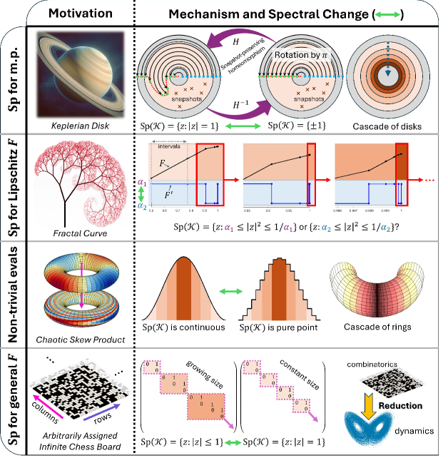
First row (lower bound for measure-preserving systems in Theorem 2.1): We consider measure-preserving dynamics on the unit disk. At each stage, we alter the dynamical system consistently with the observed data so that it is related to a rotation by a measure-preserving homeomorphism, thus drastically changing the spectrum. This alteration is executed such that the cascade of homeomorphisms and ensuing dynamical systems converge to an underlying limit, providing the adversarial family of dynamical systems.
Second row (lower bound for smooth systems in Theorem 2.1): We consider (smoothed) interval exchange maps, whose derivatives switch in a self-similar manner at the endpoints of the interval. This switching causes the approximated spectrum to alternate between different annuli.
Third row (lower bound for extremely nice systems in Theorem 2.5): We examine skew products on tori, where the spectral type depends on the existence of neighborhoods with constant cross-sections. The spectral change is centered around constructing a skew product through iterations of locally constructed piecewise constant and smooth approximations.
Fourth row (lower bound for discrete-space systems in Theorem 2.4): Here, the spectral change is more abstract since we are proving that three limits are needed. Using an infinite matrix of zeros and ones, we embed the combinatorial problem of deciding whether a matrix contains only finitely many columns with finitely many 1’s into the dynamics.
Despite its potential, practical challenges with infinite-dimensional spectral problems often limit the effectiveness of Koopman theory [27]. For instance, the projection used in dynamic mode decomposition (DMD) methods [37, 38], while serving as a catalyst for algorithms, generally fails to converge and can be unstable, even with perfect data [17, 28] (see Example 1.3 and Figure 2). While some techniques effectively learn certain spectral properties of Koopman operators [7, 39, 40, 41, 42, 43, 44, 45, 46], others like EDMD [47] seem effective but convergence is weak and achieved only along subsequences [48]. This raises a fundamental open question about when and how the robust computation of spectral properties can be ensured:
Question: When can we robustly learn the spectral properties of Koopman operators from trajectory data of dynamical systems, and when can we not?
To address this question, we develop a foundational program for Koopman operator learning that links the disparate fields of computations on infinite-dimensional Hilbert spaces, particularly the Solvability Complexity Index (SCI) hierarchy [49, 50, 51], and ergodic/dynamical systems theory. The SCI hierarchy classifies the difficulty of computational problems and proves algorithmic optimality by counting the number of successive limits required in a computation, known as towers of algorithms. These were first introduced in dynamical systems theory by Smale, who explored the dynamics of iterative rational maps for computing polynomial roots, addressing the issue that algorithms such as Newton’s method need not converge. Smale posed the question [52], “Is there any purely iterative generally convergent algorithm for polynomial zero finding?”. McMullen [53, 54] answered affirmatively for degree 3, but negatively for higher degrees. Doyle and McMullen later strikingly found that the problem could be solved for degrees 4 and 5 using towers of algorithms (successive iterations taken to infinity), but not for degree 6 or higher, no matter the tower’s height [55]. This is further detailed in McMullen’s Fields Medal citation [56]. Towers of algorithms have also resolved the “classical computational spectral problem” of computing spectra from infinite matrix coefficients [49], such as in discrete Schrödinger operators, a problem dating back to Szegő’s work on finite section approximations [57] and Schwinger’s foundational studies on Schrödinger operators [58]. We introduce new techniques that extend the SCI hierarchy and expand its applicative scope to data-driven dynamical systems.
Our program tackles upper and lower bounds within the SCI hierarchy. For upper bounds, we introduce the first learning algorithms that guarantee convergence under broad conditions, and include verification processes. Our techniques mitigate spurious eigenvalues from DMD methods by locally minimizing spectral distances. We also adapt Fourier tools from mathematical physics (the famous RAGE theorem) into towers of algorithms, introducing novel methods to the Koopman framework. For lower bounds, we establish for the first time that certain problems are unsolvable by any learning algorithms, even probabilistic ones with unlimited data (see Figure 1). This involves embedding abrupt spectral changes tied to the system’s geometry into dynamics, effectively creating families of adversarial systems where no algorithm can reliably compute spectral properties, performing no better than random chance (probability of convergence ).
Therefore, we precisely identify the barriers to robust Koopman learning and classify the complexity of these problems. We lay the groundwork for a classification theory - a toolbox - to determine which dynamical systems and Koopman spectral properties can be learned. Below are some examples of the questions we explore.
Example 1.1.
Consider the rotation on the circle , where . One might ask: Is ergodic? In other words, does
| (1) |
If we know the map symbolically, we can determine the answer ( is ergodic if and only if is irrational) in a single limit by testing the equality of with rational numbers. However, when relying solely on data from a set of observables (functions ), we require two limits. We need the time limit . Then we need a basis of functions on to verify if Equation 1 holds [59], taking the function limit . Importantly, Birkhoff’s ergodic theorem allows us to make this claim (without additional tools like RKHS), despite being a space of equivalence classes of functions, without additional tools like RKHS.
Example 1.2.
We adapt our discussion to Arnold’s circle map: where . When , we recover our previous example, where the map is not only ergodic but uniformly ergodic [60], indicating that any initial condition demonstrates ergodicity. However, for certain values of , the map loses its ergodicity for any . Here, one might explore the ergodic partition [59], which divides the space into invariant sets where dynamics remain ergodic. This analysis would necessitate a third successive limit , where an increasing number of initial conditions are sampled according to an invariant measure.
Example 1.3.
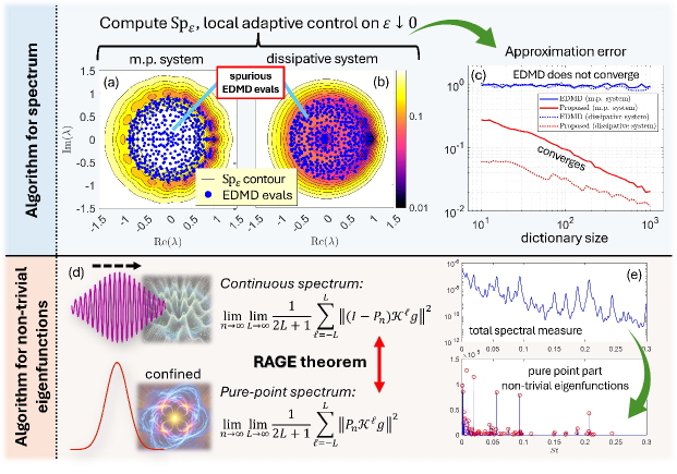
In our final example on the unit circle, we examine the doubling map: This map is measure-preserving but not invertible, and the Koopman spectrum is the unit disk. Trying to compute this spectrum via EDMD requires two successive limits: a large data limit followed by a large subspace limit . However, using a Fourier basis results in any EDMD matrix post-first limit being a direct sum of Jordan matrices and zeroes [39], yielding a spectrum of . Thus, significant regions of the spectrum are missed, and EDMD becomes exponentially unstable as . Figure 2 shows another warning example with spurious eigenvalues of EDMD.
Summary of Main Results
We consider discrete-time dynamical systems
| (2) |
Here, the statespace is a compact metric space , is the system’s state, is an unknown continuous function, and indexes time. The Koopman operator is defined via the composition formula:
| (3) |
where is a finite positive Borel measure. For our upper bounds, is general, but in our lower bounds, unless otherwise stated, will be the standard Lebesgue measure. Hence, projects state observations (with “observable” ) forward by one time step, capturing the dynamic progression of the system. The key property of is its linearity, enabling analysis based on spectral decompositions. The cost of this linearization is that acts on an infinite-dimensional function space ( here, but others are certainly possible). Our goal is to learn spectral properties of from snapshot data
| (4) |
Data may originate from long or short trajectories in experiments or simulations. This setting is central to the growing interest in using Koopman operator theory to drive practical applications of trajectory data across diverse fields.
Our results elucidate the conditions for robust Koopman learning, identify fundamental barriers to learning algorithms, and lay the foundation for a classification theory. We show (see Appendix for proofs and further problems):
-
•
Theorem 2.1: If preserves (this can be weakened) and its variation is uniformly controlled, there exists a deterministic learning algorithm that computes the spectrum of from snapshots as . Unlike EDMD, which generally fails to converge (see Example 1.3 and Figure 2), is not based on eigenvalues of a matrix discretization. However, if either of these properties of is dropped, then unless extreme assumptions are made (e.g., access to a finite-dimensional invariant subspace), no learning algorithm – deterministic or probabilistic – can converge using a single limit.
NB: Common in ML and scientific computation, we analyze sequences of algorithms indexed by , which might represent the amount of data used or the number of neural network layers. Our impossibility results are far broader, covering any type of algorithm - can index anything.
-
•
Theorem 2.3: Nevertheless, when dropping the measure-preserving and variation assumptions, it is possible to compute spectra by taking successive parameters to infinity. Convergence is achieved as for learning algorithms . This approach lays the groundwork for a classification theory that identifies the necessary number of limits for optimal Koopman learning algorithms. Using these tools, we show that one can robustly learn the spectra of Koopman operators in three limits.
-
•
Theorem 2.4: For general systems, computing spectra of from snapshots requires three successive limits, irrespective of the algorithm used. Generically, this cannot be achieved in two limits. Hence, Theorem 2.3’s algorithm is optimal.
-
•
Theorem 2.5: Finding or determining the existence of non-trivial eigenfunctions of in a single limit is impossible, even if the system is measure-preserving, invertible, and and its inverse are smooth with known bounded Lipschitz constants. However, this can be accomplished with two successive limits. This issue ties directly to the challenge of identifying finite-dimensional coordinate systems and embeddings that appear to linearize the dynamics.
The impossibility results hold even if we allow the algorithm to sample as many times as it wants to any accuracy it wants. These results are universal; no algorithm, including clever reparametrizations of a convergent procedure or enhanced neural networks, can circumvent them. As detailed in our methods section and illustrated in Figure 1, we embed sudden changes to the spectrum into the system dynamics to prevent algorithmic convergence. We establish each lower bound for basic choices of (disk, interval, torus), and the techniques extend to other and function spaces.
The use of successive limits may surprise the reader. However, unless one has very strong assumptions about the system, every convergent method for Koopman learning in the literature depends on several parameters taken successively to infinity (as it must, see Table 1). For example, could correspond to an increasing amount of snapshot data, while might correspond to an increasing number of observables . Key questions are how many limits are required and how the answer depends on the properties of the dynamical system.
2 Fundamental Barriers
In the real world, we never have access to exact snapshot data in Equation 4, which is affected by noise, measurement errors, or finite precision storage. To strengthen our impossibility results, we consider a perfect measurement device, whereby data can be approximated and stored to arbitrary precision. We assume access to the training data
This means an algorithm can sample any of the points to any desired accuracy.
Can we learn Koopman spectra?
The most fundamental spectral property of , is its approximate point spectrum:
An observable with
| (5) |
for a scalar is known as -pseudoeigenfunction and is physically relevant since
| (6) |
Hence, describes an approximate coherent oscillation and decay/growth of the observable with time. (Pseudo)eigenfunctions and encode information about the underlying dynamical system [61]. For example, they characterize the global stability of equilibria [62], and their level sets determine ergodic partitions [23], invariant manifolds [63], isostables [64].
Methods for learning (such as EDMD) face problems like spurious eigenvalues, missing parts of the spectrum and instabilities. Recent work shows how to avoid spurious eigenvalues by computing pseudospectra [44]. However, it remains an open problem whether can be computed for general systems from trajectory data. We measure convergence in the Hausdorff metric, which captures convergence without spurious eigenvalues or missing spectral regions.
Our theorems solve this problem. First, we show that we can compute from trajectory data if is measure-preserving (m.p.) (but not necessarily invertible) and we have control on its variation. We set
Here, is an increasing continuous function with , known as a modulus of continuity, that controls the variation of : for all . Since is uniformly continuous ( is compact), there is always such a modulus of continuity , but when defining we are assuming that a suitable is known across the whole considered class of dynamical systems. Theorem 2.1 also shows that if we drop these assumptions, computing is no longer possible. In particular, Theorem 2.1 shows a sharp boundary in assumptions needed for Koopman learning. We use and to denote the closed ball of radius center and the open unit disk, respectively.
Theorem 2.1.
There exists a sequence of deterministic learning algorithms using such that:
-
Convergence: ;
-
Error control: .
However, if we drop either assumption (m.p. or uniform modulus of continuity ), there is no sequence of convergent algorithms. For example, let or , where
-
•
There does not exist deterministic learning algorithms using with .
-
•
For any probabilistic learning algorithms using ,
I.e., performance is no better than random chance.
Theorem 2.1 highlights fundamental barriers regarding the existence of algorithms for Koopman learning. Despite widespread optimism and the undeniable success of applied Koopmanism, Theorem 2.1 underscores the necessity of understanding the assumptions required for the dynamical system. Our results immediately open up a classification theory on which dynamical systems and which problems allow Koopman learning. Several remarks are worth making:
-
Error control, AI, and computer-assisted proofs: The convergence in Theorem 2.1 includes error control, allowing us to bound how far the output is from the spectrum. This capability is crucial as it assures the reliability of the output for applications, including computer-assisted proofs. The significance of this field is rapidly increasing, as illustrated by the recent computer-assisted proof of the blow-up of the 3D Euler equation with smooth initial data [65], considered one of the major open problems in nonlinear PDEs, and the emerging use of neural networks in this area [66].
Example 2.2 (Example of robust Koopman learning).
As an example, the top panel of Figure 2 shows the convergence of the algorithm from the proof of Theorem 2.1 for an undamped and damped Duffing oscillator. In contrast, and in general, methods such as EDMD do not converge.
-
Beyond measure-preserving systems: In the upper bound, the measure-preserving assumption can be replaced by systems where we can control how fast the resolvent norm blows up as approaches the spectrum. Quite general estimates of this type can be obtained for finite rank operators and compact perturbations of self-adjoint and unitary operators, among others [67, 68]. These estimates can be applied to spectral Koopman operators [69, Section 2]. For example, systems with a global (Milnor) attractor of zero Lebesgue measure, where the non-unitary part acts on a domain-truncated modulated Fock space [70].
-
Randomized algorithms and training: The impossibility results in Theorem 2.1 cover randomized algorithms, including scenarios where trajectories are sampled randomly (e.g., Monte Carlo). In ML, employing a probability distribution over training data and using randomized training algorithms, such as stochastic gradient descent, is standard practice. Theorem 2.1 encompasses all these situations, and no computable probability distribution can negate these limitations.
-
Probabilistic phase transitions at : The phase transition at of the probability of success is expected in discrete mathematics. For example, if we wanted to answer a decision problem such as “Is the system ergodic?”, we could achieve a probability of success of by flipping a coin to decide “yes” or “no”. For such problems, if one could achieve a probability greater than , the probability of success can be made arbitrarily close to through repeated trials (essentially, as one would detect a biased coin). We prove that this also occurs for arbitrary computational problems (including those in continuous mathematics) in the Appendix.
-
Learning statistics is not enough: The classes and are well-behaved and allow Monte Carlo integration of integrals involving observables [71]. Hence, Theorem 2.1 shows that, even when we are capable of computing statistical properties of the dynamical system, we may not be able to learn Koopman spectra.
-
Model of computation: The algorithms can be restricted to Turing machines (digital computation) [72] or BSS machines (real number computation) [73]. However, our results are stronger than those obtained by Turing’s techniques. The impossibility results in Theorem 2.1 hold in any model of computation, even for any randomized Turing or BSS machine that can solve the halting problem.
-
Smoother and sampling derivatives do not help: The impossibility results hold even if we consider smoother and allow our algorithms to sample derivatives of .
Towers of algorithms and classifications
Despite the impossibility results of Theorem 2.1, we can learn spectra in these cases if we drop the requirement of a convergent sequence . Let
Theorem 2.3 shows that we can learn using algorithms that converge in multiple successive limits. We call these towers of algorithms. They allow us to build a classification theory that lays the foundation and mathematical language for robust Koopman learning.
Theorem 2.3.
Two limits for : There exist deterministic learning algorithms using with
| (7) |
Two limits for : There exists deterministic learning algorithms using with
| (8) |
Three limits for : There exists deterministic learning algorithms using with
The final part of Theorem 2.3 shows the remarkable result that we can robustly learn spectra of general Koopman operators for continuous . The assumption of continuity can be weakened but is natural since discontinuous can lead to pathologies such as the nonexistence of ergodic partitions [74].
The SCI for Koopman
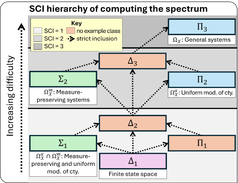
The phenomenon in Theorem 2.3 is captured by the SCI hierarchy, which classifies the difficulty of computational problems based on the smallest number of limits needed to solve them. For a class of dynamical systems and map to a metric space (e.g., mapping to the Hausdorff metric ), the SCI is the fewest number of limits needed to learn from . Hence, the final part of Theorem 2.3 says that computing has . In Theorem 2.4, we show that this is sharp (), even for discrete-space dynamical systems where one does not have to worry about the variation of . A problem lies in if it has , and it lies in if there exists a sequence of deterministic learning algorithms such that for all .
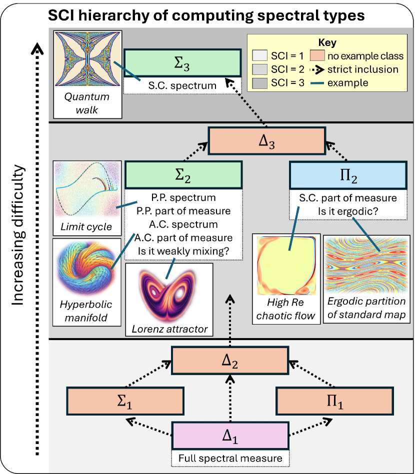
Theorem 2.3 shows more than convergence. The penultimate limit in Equation 7 is contained in the desired set, up to a controllable error. We call this , with a subscript indicating the number of limits. Similarly, the penultimate limit in Equation 8 covers the desired set, up to a controllable error. We call this . These refined classes capture the notion of verification. For example, the first part of Theorem 2.1 demonstrates convergence. Figure 3 summarizes the SCI hierarchy for computing the spectrum of Koopman operators. The SCI hierarchy also contains a calculus, allowing users to mix and match assumptions. For example, the class is in . We show the stronger result of verification - that the class is in . Similarly, Figure 4 summarizes the SCI hierarchy for determining the spectral type of systems in . Our results span various classes but represent just the beginning of a vast classification theory.
Multiple limit phenomenon in Koopman algorithms
The SCI hierarchy directly connects with the literature on algorithms that learn the spectral properties of Koopman operators. Table 1 contains convergence results in the Koopman literature and the corresponding upper bounds in the SCI hierarchy. Each algorithm comes with assumptions made about the dynamical system. Note that some of these techniques are not sharp, as they use more limits than needed.
Beyond Table 1, Dellnitz and Junge [75] exemplify multiple successive limits in data-driven dynamical systems. Their seminal work on approximating SRB measures involves three successive limits: the first is for Monte Carlo integration, the second increases the dimension of a finite-dimensional subspace to compute spectra of a compact operator, particularly the invariant measure of a randomly perturbed system, and the final limit pertains to a smoothness parameter (see their Theorem 4.4). It is common to use two successive limits when using Ulam’s method to approximate isolated eigenvalues of quasicompact Perron–Frobenius (the pre-dual of the Koopman operator), corresponding to Monte Carlo approximation and finite matrix size, respectively [76, 77, 78], see also the Fourier scheme in [79]. Ulam’s method need not always converge (see [80, Section 2.6] for an example of spectral pollution), which can often be rectified by smoothing with noise [80]. In some situations, it is also possible to adaptively choose the size of this noise based on the partition diameter to ensure a two-limit process [80, Theorem 4]. As in some of the classes considered in this paper, one can reduce the number of successive limits if one can control the quadrature error. The same remarks for EDMD in Table 1 hold for related data-driven dimension reduction techniques for dynamical systems [81]. For multiple successive limits in control, see [82, Theorem 3].
| Algorithm | Comments/Assumptions | Spectral Problem’s Corresponding SCI Upper Bound | |||
|---|---|---|---|---|---|
| KMD | Spectrum | Spectral Measure (if m.p.) | Spectral Type (if m.p.) | ||
| Extended DMD [47] | general spaces | N/C | N/C | n/a | |
| \hdashline[0.5pt/1pt] Residual DMD [44] | general spaces | varies, see [84] | |||
| e.g., a.c. density: | |||||
| \hdashline[0.5pt/1pt] Measure-preserving EDMD [45] | m.p. systems | N/C | (general) | n/a | |
| (delay-embedding) | |||||
| \hdashline[0.5pt/1pt] Hankel DMD [85] | m.p. ergodic systems | N/C | N/C | n/a | |
| \hdashline[0.5pt/1pt] Periodic approximations [86] | m.p. a.c. | N/C | (see [87]) | a.c. density: | |
| \hdashline[0.5pt/1pt] Christoffel–Darboux kernel [40] | m.p. ergodic systems | n/a | e.g., a.c. density: | ||
| \hdashline[0.5pt/1pt] Generator EDMD [88] | cts.-time, samples | N/C | (see [89]) | n/a | |
| (otherwise additional limit) | |||||
| \hdashline[0.5pt/1pt] Compactification [42] | cts.-time, m.p. ergodic systems | N/C | n/a | ||
| \hdashline[0.5pt/1pt] Resolvent compactification [43] | cts.-time, m.p. ergodic systems | N/C | n/a | ||
| \hdashline[0.5pt/1pt] Diffusion maps [90] (see also [10]) | cts.-time, m.p. ergodic systems | n/a | n/a | n/a | |
These examples provide upper bounds. A key question in algorithm design for each method is whether they are optimal. Can convergence be achieved with fewer limits, and if not, what assumptions about the system are necessary to make it easier? Addressing this requires proving lower bounds, as we do in this paper. Establishing computational boundaries involves various techniques for constructing convergent algorithms (upper bounds) and proving impossibility results (lower bounds), depending on the type of dynamical system and the quantities we aim to compute.
General systems require three limits
Theorem 2.3 shows that the spectra of general Koopman operators can be computed using three limits (). We establish that this is optimal; for general systems, computing inherently requires three limits ().
Let (or any countable discrete space), equipped with the usual counting measure , and consider dynamical systems governed by a nonlinear function . Such discrete-space systems are well studied since they are often conjugate to chaotic systems on continuous spaces; hence, we may also translate computational problems and classifications to continuous spaces. The Koopman operator acts on sequences via
We consider as an operator on , and assume that it is bounded. Let
and consider the training set corresponding to discrete samples of .
Theorem 2.4.
The problem of learning from for lies in and has . That is, we can learn in three successive limits but not two.
Learning non-trivial eigenpairs is very hard, even for simple well-behaved systems
As a final problem, we consider whether we can learn non-trivial eigenvalues and eigenfunctions. This question is often the focus of research in applied Koopmanism and corresponds to finding a coordinate system in which the dynamics are (or appear) linear. The constant function is an eigenfunction with eigenvalue but is trivial and contains no dynamical information. An eigenfunction is non-trivial. A system is weakly mixing precisely when there are no non-trivial eigenfunctions. We let denote the closure of the set of eigenvalues of , i.e., the so-called pure point spectrum.
Theorem 2.5 shows that computing non-trivial eigenfunctions is impossible in one limit, even with randomized methods, if and are smooth functions with a known Lipschitz constant, and the statespace is as simple as a torus.
Theorem 2.5.
Consider the torus and
There are no learning algorithms (deterministic or probabilistic with success probability ) using with
There are no learning algorithms (deterministic or probabilistic with success probability ) using with
However, both problems lie in (two limits with verification).
This result immediately explains why obtaining finite-dimensional coordinate systems and embeddings (e.g., autoencoders and latent space representation) in which the dynamics are linear is a considerable challenge. Instead, one must settle for approximate pseudoeigenfunctions as in and Equation 6, for which the problem is (see Figure 3). Our -tower depends on two parameters: a time lag for auto-correlations (the number of data points depends adaptively on this) and a sequence of increasing projections onto finite-dimensional subspaces (according to a dictionary). Theorem 2.5 proves this is optimal - no one limit procedure for detecting or computing non-trivial eigenvalues exists.
Example 2.6.
The bottom panel of Figure 2 shows the application of the -tower for extracting non-trivial eigenvalues of a high Reynolds number cavity flow with mixed spectral type. The two limits are motivated by the so-called discrete-time RAGE theorem from mathematical physics [91], which is a consequence of Wiener’s classical lemma, which relates the asymptotic behavior of Fourier coefficients of a measure to its atomic part.
3 Discussion
We have developed a framework that reveals both the potential and the limitations of applying Koopman operators in the data-driven analysis of dynamical systems. Our results include upper bounds (algorithms with guaranteed convergence and verification) and, for the first time, lower bounds (impossibility theorems) for robust Koopman learning. Through several key theorems, we reveal the conditions under which the spectral properties of Koopman operators can be robustly learned, and we identify scenarios where learning is inherently impossible. Our lower bounds and techniques can easily be generalized to other dynamical systems. Specifically, we uncover the exact barriers to learning spectral properties, such as detecting non-trivial eigenfunctions.
This study introduces successive limits and the SCI hierarchy to applied Koopmanism, offering a classification for the computational and learning challenges present in dynamical systems. The hierarchy is shown in Figures 3 and 4 for computing spectra and spectral type, respectively. This approach not only paves the way for applying Koopman operator theory to real-world problems but also confirms that the spectral properties of these operators can be learned under suitable conditions. It encompasses all previous convergence results in the literature, now providing a unified language for developing lower bounds and proving optimality.
Our results are only the start of traversing the boundaries of robust Koopman learning and developing a theory of necessary and sufficient conditions. Future problems amenable to our techniques include:
-
•
Dealing with other spaces of observables than . This also useful for transfer operators that act on distributions. A key question is whether the difficulty of a computational problem (and whether it can even be solved) changes with the function space.
-
•
Cases where we only have partial observations of the system instead of the full snapshots in Equation 4.
-
•
Koopman generators for continuous-time systems.
-
•
What are the boundaries of Koopman control? E.g., our upper bounds open the door to verified control.
-
•
What are the boundaries for learning other objects, such as invariant measures of the system?
-
•
Beyond eigenvalues and spectra, what are the boundaries of learning the spectral type of Koopman operators? Some of these problems are extremely difficult - in the Appendix, we give an example where determining whether a system is ergodic has .
The techniques of this paper may have applications in other areas of scientific computation in ML. For example, recent results show that it is possible to learn elliptic PDEs from training data consisting of pairs of random forcing terms and corresponding solutions [92]. This is similar in spirit to the snapshot setting of learning Koopman operators. It is currently unknown whether hyperbolic PDEs can be learned, and our proof techniques could shed light on this problem.
4 Methods
For lower bounds (impossibility results), we embed specific phase transitions of the spectral properties of into the dynamics, ensuring they are consistent with the sampled training (trajectory) data. To prove , we proceed by contradiction, assuming that a convergent sequence of algorithms exists. We construct an adversarial family of dynamical systems, taking into account the probability of success, to ensure that convergence cannot occur with a probability greater than . To prove , we embed specific combinatorial problems from descriptive set theory into the dynamics. Each lower bound we establish depends on different phase transitions, as detailed in Figure 1, where we also motivate each phase transition. This proof method systematically links the foundations of computation with classical ergodic theory and can be extended to problems beyond those considered in this paper.
We also extend the mathematics behind the SCI hierarchy in several directions, including going beyond the matrix viewpoint to approximation theory and sampling the function , as well as the allowance for sequences of probabilistic algorithms. (See the concept of a sequence of probabilistic general algorithms we develop and the proven structure theorems in the Appendix.) These tools enable us to prove impossibility results in any model of computation while capturing concepts such as adaptive and probabilistic sampling of the function .
The construction of algorithms for upper bounds depends on the spectral problem. To compute the spectrum, we provide a general scheme for arbitrary compact metric spaces and Borel measures . This involves building a suitable dictionary and using it to approximate the function . Similar in spirit to a barrier function (used to guide optimization algorithms), this function vanishes on the spectrum and increases as moves further away from . We then locally minimize this function to approximate spectra. A crucial component is generalizing and extending the techniques of ResDMD, which employed a Galerkin approximation of using trajectory data to approximate pseudospectra (level sets of ). This approach allows us to rigorously approximate from above with locally uniform convergence while avoiding issues such as spurious eigenvalues. We show how this leads to the sharp upper bounds shown in Figure 3 for different classes of dynamical systems. In contrast to DMD methods, our techniques do not rely on computing eigenvalues of a matrix discretization of . To compute non-trivial eigenfunctions, we use the RAGE theorem to compute the pure point part of spectral measures of observables. We use these approximations across different observables and a nest of dyadic spectral intervals to filter out the pure point spectrum (eigenvalues).
Appendix of Supplementary Material
Here, we provide proofs of theorems, and detailed explanations of the experimental setup. These results are briefly summarized as follows, and extend upon the theorems presented in the main text:
-
•
Theorem B.1: As a warm-up, for continuous, measure-preserving and invertible maps on the unit circle, the SCI of computing the spectrum is 1, the SCI of determining ergodicity is 2, and after dropping the assumption of continuity, the SCI of computing the spectrum is .
-
•
Theorem B.6: For general statespace , the SCI of computing the spectrum of measure-preserving systems with uniformly bounded modulus of continuity is , the SCI of computing the spectrum of measure-preserving systems is , the SCI of computing the spectrum of systems with uniformly bounded modulus of continuity is , the SCI of computing the spectrum of continuous systems is .
-
•
Theorem B.9: For continuous, measure-preserving and invertible maps on the unit disk, the SCI of computing the spectrum is 2, i.e., controlling the variability of cannot be dropped if we want to compute the spectrum in one limit.
-
•
Theorem B.14: For smooth, invertible maps on the unit interval, with uniformly bounded derivatives (for and ), the SCI of computing the spectrum is 2, i.e., the measure-perserving condition cannot be dropped if we want to compute the spectrum in one limit.
In all of the above theorems, we also prove the relevant or classifications.
Appendix A Background
This section provides background information regarding Koopman operators and the Solvability Complexity Index (SCI) for the proofs. We end this section by discussing the paper’s setup.
A.1 Koopman operators
Throughout, we consider discrete-time dynamical systems:
Here, denotes the state of the system, and the metric space denotes the statespace. Often, , though this is not required in what follows (unless explicitly stated). The function governs the evolution of the dynamical system and is generally nonlinear. (Here, we mean that is linear if is a vector space and is linear. Otherwise, we call nonlinear.) We lift the system into a (typically infinite-dimensional) vector space of observable functions using a Koopman operator to deal with the nonlinearity. A Koopman operator [21, 22] is defined on a Banach space of functions , where the functions are referred to as observables and measure the state of the system. Koopman operators allow us to study the evolution of observables in through a linear framework. The Koopman operator is defined via the composition formula:
were is a suitable domain. This definition means that represents the measurement of the state one time-step ahead of , and hence that effectively captures the dynamic progression of the system.
The critical property of the Koopman operator is its linearity. This linearity holds irrespective of whether the map in Equation 2 is linear or nonlinear. Consequently, the spectral properties of become a powerful tool in analyzing the dynamical system’s behavior. The Koopman operator is not defined uniquely by the dynamical system in (2), but fundamentally depends on the space . Throughout, we focus on the choice
for some positive measure .111We do not assume that this measure is invariant. For Hamiltonian systems, a common choice of is the standard Lebesgue measure, for which the Koopman operator is unitary on . For other systems, we can select according to the region where we wish to study the dynamics, such as a Gaussian measure. In many applications, corresponds to an unknown ergodic measure on an attractor. In going from a pointwise definition in (3) to the space , a little care is needed since consists of equivalence classes of functions. We assume that the map is nonsingular with respect to , meaning that
This ensures that the Koopman operator is well-defined since for -almost every implies that for -almost every . The pushforward measure is defined as , and the fact that is nonsingular with respect to is equivalent to saying that is absolutely continuous with respect to . We assume that is a bounded linear operator on the Hilbert space . This assumption is equivalent to saying that the Radon–Nikodym derivative lies in . The above Hilbert space setting is standard in the Koopman literature, though our results can be extended to other function spaces such as those studied in [70]. Once are specified, we let denote the corresponding Koopman operator on the corresponding Hilbert space .
Since acts on an infinite-dimensional function space, we have exchanged the nonlinearity in (2) for an infinite-dimensional linear system. This means that the spectral properties of can be significantly more complex than those of a finite matrix, making them more challenging to compute. A message of this paper is that, in most cases, unless strong assumptions are made regarding the system, the spectral properties of are impossible to compute in a single limit, even if we had a perfect measurement device to sample trajectories of the dynamical system.
A.1.1 Koopman spectrum
If is an eigenfunction of with eigenvalue , then exhibits perfect coherence222Coherence here is meant in the sense of an observation for which all the points in state space exhibit the same, (complex) exponential, time-dependence. since
| (9) |
The oscillation and decay/growth of the observable are dictated by the complex argument and absolute value of the eigenvalue , respectively. In infinite dimensions, the appropriate generalization of the set of eigenvalues of is the spectrum:
Here, denotes the identity operator. In contrast to finite matrices, the spectrum may contain points that are not eigenvalues in addition to eigenvalues. This phenomenon occurs because there are more ways for to not exist in infinite dimensions than in finite dimensions. For example, the standard Lorenz system on the Lorenz attractor has a Koopman operator with no nontrivial eigenvalues [93]. The approximate point spectrum is
and for , the approximate point pseudospectrum is
An observable with and for is known as -pseudoeigenfunction. Such observables satisfy
In other words, describes an approximate coherent oscillation and decay/growth of the observable with time. The (pseudo)eigenfunctions and encode information about the underlying dynamical system [61]. For example, the level sets of certain eigenfunctions determine ergodic partitions [59, 23], invariant manifolds [63], isostables [64], and the global stability of equilibria [62] can be characterized by pseudoeigenfunctions and .
In this paper, we will focus on the computation of . We anticipate that further foundational results can be proven on the computation of other spectral properties of Koopman operators, such as spectral type. For example, see Theorem B.19 regarding the detection of non-trivial eigenfunctions.
Two special classes of Koopman operators are defined as follows:
-
•
Measure-preserving systems: The dynamical system preserves if and only if is an isometry, that is .
-
•
Measure-preserving invertible systems: The dynamical system preserves and is invertible modulo -null sets [94, Chapter 7] if and only if is unitary, that is .
Note that if is an isometry, but not unitary, then the spectrum of is the unit disc and . If is unitary, then the spectrum of is equal to and is a subset of .
A.2 The Solvability Complexity Index – classifying the difficulty of problems
We now outline the fundamentals of the Solvability Complexity Index Hierarchy. This tool allows us to precisely classify the difficulty of computational problems and prove that algorithms are optimal, realizing the boundaries of what is possible. We give the definitions of the hierarchy before specializing to the computational setup of this paper, where we give a precise formulation of a perfect measuring device.
A.2.1 Computational problems and general algorithms
Before classifying the difficulty of computational problems, we must precisely define what a computational problem means. Precision here is essential since altering the information an algorithm is permitted to use can significantly affect the difficulty of a problem or even whether the problem can be solved at all. The following definition of a computational problem is deliberately general, designed to encompass all types of problems encountered in computational mathematics. For example, as well as spectral problems, the SCI hierarchy has been applied to other areas of mathematics, including PDEs [95, 96], the limits of AI, and Smale’s 18th problem [97], and optimization [98].
Definition A.1 (Computational problem).
The basic objects of a computational problem are:
-
•
A primary set, , that describes the input class;
-
•
A metric space ;
-
•
A problem function ;
-
•
An evaluation set, , of functions on .
The problem function is the object we want to compute, with the notion of convergence captured by the metric space . The evaluation set describes the information that algorithms can read. We require that separates elements of to the degree of separation achieved by :
| (10) |
In other words, any is uniquely determined by the set of evaluations (otherwise it is impossible to recover from ). We refer to the collection as a computational problem.
Example A.2.
In the above setting of dynamical systems, we can fix the metric space and the measure . The primary set could be a class of functions , each of which induces a dynamical system with bounded on . The problem function could describe a spectral property of . For example, we could consider the computation of the approximate point spectrum with . Since is bounded, is a compact subset of . Hence, we let be the Hausdorff metric. The Hausdorf metric space, , is the collection of non-empty compact subsets of equipped with the Hausdorff metric:
Convergence to the spectrum in this metric means our algorithms converge without spectral pollution (persistent spurious eigenvalues) or spectral invisibility (missing parts of the spectrum). As our evaluation set, we could consider maps for or a subset of such . For example, if , then is a real vector-valued function.
With the definition of a computational problem established, we now define what we mean by an algorithm. An algorithm is a function that, unlike the problem function , utilizes the evaluation set in some manner. The specifics of how is used (or even which sets of are permitted) depend on the computational model. We adopt a general definition for proving lower bounds (impossibility results). This approach not only yields stronger results but also significantly simplifies the proofs. Specifically, we aim to establish lower bounds that are valid in any model of computation.
Definition A.3 (General algorithm).
Given a computational problem , a general algorithm is a map such that ,
-
1.
There exists a non-empty finite subset of evaluations ;
-
2.
The action of on only depends on ;
-
3.
If with for every , then and .
Definition A.3 outlines the most fundamental properties of any reasonable deterministic computational device:
-
•
The first property says that can only use a finite amount of information, though it can adaptively choose this information as it processes the input.
-
•
The second property ensures that the output of depends solely on the information it has accessed.
-
•
The final property ensures that produces outputs and consistently accesses information. Specifically, if sees the same information for two different inputs, it must behave identically for those two inputs.
A general algorithm has no restrictions on the operations allowed. It is more powerful than a Turing machine [72] or BSS machine333Blum–Shub–Smale (BSS) machines are a model of computation designed to work over any ring or field, most notably over the real numbers. This distinguishes them from Turing machines, which are based on discrete values. A BSS machine extends the concept of computation to include computation with real numbers and other continuous data. One should think of a BSS machine as akin to an algorithm that deals with exact arithmetic. [73] and serves two main purposes:
-
(i)
A focus on what really matters: Definition A.3 significantly simplifies the process of proving lower bounds. The non-computability results we present stem from the intrinsic non-computability of the problems themselves, not from the type of operations allowed being too restrictive. Specifically, the limitation lies in the algorithmic input being inadequate for solving the problem.
-
(ii)
Classifications with the strongest possible lower and upper bounds: The generality of Definition A.3 implies that a lower bound established for general algorithms also applies to any computational model. Furthermore, the algorithms we provide can be executed using only arithmetic operations, both in the Turing and BSS models. Therefore, we derive the strongest possible lower and upper bounds simultaneously.
A.2.2 Towers of algorithms
Having established precise definitions for a computational problem and a general algorithm, we now introduce the concept of a tower of algorithms. This captures the observation in the main text that algorithms for data-driven Koopmanism depend on several parameters that must be taken to successive limits to ensure convergence.
Definition A.4 (Tower of algorithms).
Let . A tower of algorithms of height for a computational problem is a collection of functions
where are general algorithms (Definition A.3) and for every , the following convergence holds in :
We shall use the term “tower” even if .
When we prove upper bounds (i.e., provide algorithms that solve a problem), we can specify the type of tower by imposing conditions on the functions at the lowest level. In essence, the type is the toolbox allowed:
-
•
A general tower, denoted by , refers to Definition A.4 with no further restrictions.
-
•
An arithmetic tower, denoted by , refers to Definition A.4 where each can be computed using and finitely many arithmetic operations and comparisons. More precisely, if is countable, each output is a finite string of numbers (or encoding) that can be identified with an element in , and the following function is recursive444By recursive, we mean the following. If for all , , then can be executed by a Turing machine that takes as input, and that has an oracle tape consisting of . If for all , , then can be executed by a BSS machine that takes , as input, and that has an oracle that can access any for .:
We can now define the Solvability Complexity Index (SCI).
Definition A.5 (Solvability Complexity Index).
A computational problem has Solvability Complexity Index with respect to type , written , if is the smallest integer for which there exists a tower of algorithms of type and height that solves the problem. If no such tower exists, then If there exists an algorithm of type with , then .
The SCI induces the SCI hierarchy as follows.
Definition A.6 (SCI hierarchy).
Consider a collection of computational problems and let be the collection of all towers of algorithms of type . We define the following subclasses of :
In summary, a problem can be computed in successive limits, and a problem can be computed in one limit with complete error control. The in the definition of is arbitrary; replacing it with any sequence converging to zero and computable from does not alter the definition.
A.2.3 Inexact input
So far, we have only discussed algorithms with exact input from the evaluation set . However, in practice, we may only have access to input of a certain accuracy. Suppose we are given a computational problem with evaluation set , for some index set and metric space . Obtaining may be a computational task in its own right. For instance, could be the number or an inner product that is approximated using quadrature. Alternatively, it may be the case that we can only measure to a certain accuracy due to effects such as noise. In the context of Koopman operators, any physical measurement device will have a non-zero measurement error.
Hence, we cannot access , but rather with . Alternatively, just as for problems high up in the SCI hierarchy, we could need several successive limits to access . In particular, we may only have access to functions such that
| (11) |
with convergence in . We may view the problem of obtaining as a problem in the SCI hierarchy. A -classification would correspond to access of such that
| (12) |
We want algorithms that can handle all possible choices of inexact input. We can make this precise by replacing the class by the class of suitable evaluation functions that satisfy Equation 11 or Equation 12. This viewpoint is well-defined since Equation 10 holds.
Definition A.7 (Computational problems with -information).
Given and a computational problem , the corresponding computational problem with -information is denoted by and defined as follows:
-
•
The primary set is the class of tuples where , and Equation 11 holds;
-
•
The problem function is , which is well-defined by Equation 10;
-
•
The evaluation set is , where .
Similarly, the corresponding computational problem with -information is denoted by and defined as follows:
-
•
The primary set is the class of tuples where , and Equation 12 holds;
-
•
The problem function is , which is well-defined by Equation 10;
-
•
The evaluation set is , where .
For any , the SCI hierarchy given -information is then defined in an obvious manner.
The most important case of this definition is -information, which captures the notion of algorithms being robust to noise. We can also connect -information to the Turing and BSS models. For example, in the Turing case, we could enforce that each maps to and view these evaluation functions as an infinite input tape.
A.2.4 Refinements that capture error control
When performing numerical computations, particularly in many spectral applications, determining the accuracy of the results is essential. The importance of error bounds extends beyond science and engineering and holds in pure mathematics, especially when using spectral problems in computer-assisted proofs. For instance, even when a discretization method for computing spectra through eigenvalues converges, typically, only a subset of the numerically computed eigenvalues is reliable. Note that such a problem is not computable in the classical Turing sense but instead verifiable. Most infinite-dimensional spectral problems do not lie in [51], but many lie in the following refinements that capture error control [99, 100]. Classifying when error bounds can or cannot be obtained is a fundamental challenge in dealing with infinite-dimensional spectral problems.
Sufficient structure in enables two types of verification or error control: convergence from above and below. In this paper, there are two metric spaces that we use for computational problems :
-
•
If with the discrete topology, we call the problem a decision problem and denote this space by . For an input , we interpret the output as “Yes” and the output as “No”.
-
•
The Hausdorff metric space, , is suitable for computing spectra of bounded operators. It is the collection of non-empty compact subsets of equipped with the Hausdorff metric:
(13) As noted above, we are interested in the Hausdorff metric since convergence to the spectrum in this metric means that our algorithms converge without spectral pollution or spectral invisibility.
We now define notions of error control for these two metric spaces. When is a totally ordered set with relation , such as or , convergence from above or below is straightforward to define.
Definition A.8 ( and classes for totally ordered sets).
Consider a collection of computational problems and let be the collection of all towers of algorithms of type . Suppose that is a totally ordered set. We set and for , define
where and denote convergence from below and above, respectively. In other words, we have convergence from below or above in the final limit of the tower of algorithms.
The following two examples discuss and , respectively.
Example A.9 (Spectral radius of normal operators).
Let be the class of bounded normal operators on , , and consider the spectral radius problem function For normal operators, . Hence, we let be an approximation of to accuracy from below, where is the orthogonal projection onto . and hence . This classification means that for any finite , we obtain a lower bound for the value . However, we may not know how close is to and one can also show that . To see why, suppose for a contradiction that . Hence, there exists a general algorithm such that for all . We may choose such that the number of zeros in the diagonal of ensures that (this follows from the consistency requirement in the definition of a general algorithm). But then , a contradiction. The point is that we cannot compute an upper bound on from a finite amount of information, and hence, we cannot get full error control in the metric space .
Example A.10 (Is the spectral radius larger than one?).
Consider the setup of Example A.9, but now let be the decision problem, ‘Is ?’ Let be as before, then if (yes), for some , otherwise for all . Note that we have used the fact that is a -tower for the problem in Example A.9. It follows that
provides a -tower for . Again, one can show that . If we changed the decision problem to ‘Is ?’, we would obtain a classification instead.
More generally, the classes and in Definition A.8 allow verification. For example, suppose that we have a problem function and we wish to verify a theorem for some . If there exists a -tower for the problem and the theorem is true for the given , then for sufficiently large . We can compute for various and as soon as , we know that and have verified the theorem. Note, however, that we cannot use a -tower to negate such a theorem (but can, instead, use a -tower if it exists). We can only verify one way using a -tower. Similar remarks hold for .
While Definition A.8 is straightforward, it does not carry over to the more complicated Hausdorff metric. To define convergence of to in the Hausdorff metric “from below”, a first attempt may be to require that . However, this is severely restrictive. For example, when computing , we can rarely ensure that a point is exactly in . Nevertheless, we can often ensure that is close to and measure how close. Hence, it is natural to relax the condition to
The exact form of the sequence does not matter. What matters is that we can control the proximity of to being contained within using a known sequence that converges to zero as . Based on this discussion, the following provides the generalization of Definition A.8.
Definition A.11 ( and classes for Hausdorff metric).
Consider a collection of computational problems and let be the collection of all towers of algorithms of type . Suppose that is the Hausdorff metric. We set and for , we define
These classes capture convergence from below or above, up to a small error parameter . It is precisely the classes and that allow computations with verification, used, for example, in computer-assisted proofs. For example, to build a algorithm in the case of the Hausdorff metric, it is enough to construct a convergent tower such that with some computable that converges to zero.
A.2.5 Randomized algorithms
We also consider sequences of probabilistic general algorithms, which are more general than a sequence of probabilistic Turing [101, Ch. 7] or probabilistic BSS [73, Ch. 17] machines. It is common to use randomized algorithms in machine learning and optimization.555For Turing machines, it is unknown whether randomization is beneficial from a complexity class viewpoint [101, Ch. 7]. This is not the case for BSS machines [73, Ch. 17] (but it is an open problem whether any probabilistic BSS machine can be simulated by a deterministic machine having the same machine constants and with only a polynomial slowdown). However, randomization is extremely useful in practice. For example, in the context of Koopman operators, it is common to apply Monte Carlo methods that randomly sample the snapshots. We consider the following definition.
Definition A.12 (A sequence of probabilistic general algorithms).
Let be a computational problem. A sequence of probabilistic general algorithms (SPGA) is a sequence of general algorithms using with the additional properties that given an input :
-
1.
(Coin flips) Each has access to an oracle (viewed as an input appended to ) that, when queried, gives the answers or at random, each with probability ;
-
2.
(Always halts) Each halts with probability ;
-
3.
(Access to previous outputs) has access to the oracle queries that produces upon input for any .
These conditions hold for any standard probabilistic machine (e.g., Turing or BSS) and model machines that flip coins.666One could also consider other, even continuous, probability distributions. In the case of BSS machines, machines that can pick numbers uniformly at random in are no more computationally powerful [73, Section 17.5]. Hence, we do not consider such scenarios, which are also unrealistic in practice.
Remark A.13 (The reason for part 3 of Definition A.12).
It may appear that part 3 of Definition A.12 strengthens the requirements for algorithms, potentially weakening our lower bounds. However, this is not the case. If is a sequence of general algorithms that satisfies conditions 1 and 2 of Definition A.12, then there is a corresponding SPGA that also satisfies condition 3. Specifically, each ignores the additional input information in part 3 and simply runs . Therefore, part 3 of Definition A.12 enlarges our class of algorithms, strengthening our lower bounds. For example, to illustrate the use of part 3, suppose we have a decision problem (where the answer is either “Yes” or “No”). If each flips a coin to output “Yes” or “No”, the sequence fails to converge with probability 1. However, if for is allowed to output the same answer as (as permitted by part 3 of Definition A.12), the probability that is the correct answer is now .
We can now make sense of probabilistic classes in the SCI hierarchy.
Definition A.14.
A computational problem does not belong to if for any SPGA ,
A computational problem does not belong to if for any SPGA ,
The following lemma shows that implies . In other words, being limit computable by an SPGA is weaker than being limit computable by a sequence of general algorithms. Similarly, implies . Hence, at various points, we prove statements of the form , which imply the corresponding results .
Lemma A.15.
Let be a computational problem. If , then . If , then .
Proof A.16.
The proof is trivial. We prove the contrapositive. Suppose first that with a -tower solving the problem. Then is an SPGA with for any . This shows the second part of the lemma. The proof of the first part is analogous.
One may wonder why we chose in Definition A.14. The reason is that if we had chosen any number greater than instead, this number could be made arbitrarily close to when defining the classes and . This is a standard argument for Turing machines and decision problems. However, the following shows (the non-trivial and perhaps surprising result) that it also holds for arbitrary computational problems and SPGAs.
Lemma A.17.
Let be a computational problem and with .
-
•
If there exists an SPGA with
then there exists another SPGA with
-
•
If there exists an SPGA with
then there exists another SPGA with
In other words, the probability of success can be made arbitrarily close to , and hence, success can be achieved with overwhelming probability.
Proof A.18.
We prove the first statement, and the second is analogous. Suppose then that is an SPGA with
Given the SPGA and input , we run independent copies of and label these as . For , we consider the objective function defined for as
Let be such that . We may choose so that is as SPGA. Let be the event that at least of satisfy
Suppose that occurs and let . Without loss of generality, we may assume that
It follows that
Moreover, by the pigeonhole principle, there exists with
It follows that
We can now define where is chosen so that . It remains to show that we may choose sufficiently large so that .
Let be the random variable
Each is an independent Bernoulli random variable with parameter . Let . Then is a binomially distributed random variable with parameters and and
Since , it follows that we can choose large so that using standard bounds for the tail of the binomial distribution.
A.3 The setup of this paper - a perfect measurement device
In this paper, we consider computational problems where:
-
•
is a class of dynamical systems, or , on some statespace as in (2);
-
•
, the evaluation set, will be pointwise evaluations of the function :
Here, is a suitable subset of for which we allow pointwise evaluations of .
-
•
The metric space will be either , in the case of decision problems, or , when we compute spectral sets.
This setup agrees with the usual “snapshot” setting of data-driven Koopmanism where one is given access to a finite collection of pairs
However, our lower bounds become stronger. Specifically, this strengthening occurs when we prove lower bounds for a computational problem , which we remind the reader, corresponds to allowing arbitrary precision of the evaluation set according to Definition A.7. Hence, our lower bound holds even if we allow algorithms arbitrarily many point samples of to arbitrary precision. When proving lower bounds, we will always deal with the case that is the natural Lebesgue measure on , though many of our results can be easily extended to other measures.
Appendix B Statement of Theorems and Results
With the above preliminaries covered, we can now provide precise statements of our theorems.
B.1 Measure-preserving maps on the unit circle
As a simple first example, we consider the well-studied class of measure-preserving maps on the unit-circle [102, Chapter 3, Section 3], which we view as the periodic interval through standard angular coordinates. These classes are of particular importance in dynamical systems theory, and many important nonergodic dynamical systems have phase spaces that split into invariant tori. Consider the primary set
where is equipped with the standard (normalized) Lebesgue measure. The Koopman operator associated with any of the dynamical systems in is unitary. We take . We consider the problem of computing the spectrum in the Hausdorff metric:
We also consider the problem of deciding whether the dynamical system is ergodic. This second computation problem has the following problem function
Theorem B.1.
Given the above setup, we have the following classifications:
-
(a)
The spectrum can be computed in one limit, but full error control is impossible,
-
(b)
Ergodicity can be determined in two limits but not one,
-
(c)
If we remove the condition that is continuous from to define
then the SCI of the problem is infinite,
Proof B.2.
Before proving each classification, note that the maps are precisely those of the form
for some , where denotes the angular coordinate. Furthermore, the Fourier basis diagonalizes . The spectrum of is pure point and is the closure of the set of eigenvalues of :
In particular, if is rational, the spectrum consists of a finite number of points on the unit circle, whereas if is irrational, the spectrum is the entire unit circle. The conditions for ergodicity are analogous, with [103, Theorem 1.8]
With these basic facts, we can now prove the classifications in Theorem B.1.
Step 1: . Suppose for a contradiction that is an SPGA for such that
For , let be the map
and let denote a collection of maps such that
The evaluation set is , whereas the evaluation set with -inexactness, , is the set of maps , , . In particular, given , from Definition A.12 of an SPGA and Definition A.7 of -information, there exists a finite subset such that
We may choose sufficiently small irrational such that we may also choose so that
We consider running for the two inputs and (with independent calls to the oracles). Let and be the corresponding outputs, which are random variables. Note that , whereas .
For or , let be the event . By part (iii) of Definition A.3 and by Definition A.12, It follows that . Let and be the events for and , respectively. If occurs, then the law of and are the same. Hence,
Since it follows from the triangle inequality that
Hence,
This is a contradiction for sufficiently small .
Step 2: . An arithmetic algorithm with access to the point values of may compute to any specified accuracy. In particular, we let be an approximation of the set
Such a set can be computed using finitely many arithmetic operations and comparisons using the specified -information. Note that and that .
Step 3: . Suppose for a contradiction that is an SPGA for such that
For a sequence of integers with and , define the quantities
In other words,
The number has a non-terminating and non-repeating (since ) decimal expansion, and hence it is irrational so that . On the other hand, for all . We will choose the inductively to gain a contradiction, thus proving the result.
Suppose that we have defined . By our assumption,
It follows that there exists such that
Since only has -information, given any , there exists with such that the law of the output depends only on the first digits of with probability at least . Choosing sufficiently small, we can ensure that
Let be large enough so that agrees with in the first decimal places, and let be the random variable . By Definition A.12 of an SPGA and Definition A.3,
We may assume without loss of generality that . Now let be the event and note that . By our initial assumption,
Since , there must exist some with , the required contradiction.
Step 4: . We may list the rationals in without repetition as . Given an input , we let be an arithmetic algorithm with -information such that We then define
and set
It is clear that
Moreover, since if and only if is irrational, converges to from above.
Step 5: . We prove this result for exact input instead of -information (which also implies the result for -information). Suppose for a contradiction that is a height- tower of general algorithms for . For the input , the base algorithms only ever point sample at a countable number of points as vary. We can define
where is irrational. Note that this map is measure-preserving and invertible modulo null sets. It follows from part (iii) of Definition A.3 that . In particular,
which is absurd.
Remark B.3.
Interestingly, a constructive computational procedure exists for part (b) of Theorem B.1. The constructive ergodic partition theorem first proven in [59] and expanded on in [104] and [7] applies to continuous dynamical systems on compact metric spaces. That result implies that if every element of a basis of continuous functions in (see below for the existence of such a basis) has a constant time average almost everywhere, then the dynamical system is ergodic. Two limits are necessary for this computation: the limit of the number of iterations of the dynamical system going to infinity and the limit of the number of functions in the basis going to infinity.
B.2 A general computational result providing upper bounds
In this section, we let be a compact metric space and a finite Borel measure on . Under these assumptions, there are two key properties of that we shall make use of:
-
•
is a separable Hilbert space [105, Proposition 3.4.5];
-
•
The space of continuous functions on , denoted , is dense in [106, Proposition 7.9].
In particular, by the Gram–Schmidt process, there exists an orthonormal basis of .
Definition B.4.
Let be an increasing continuous function with . We say that a continuous function has a modulus of continuity if
| (14) |
Since is compact, any continuous function is uniformly continuous and hence has a choice of so that Equation 14 holds. However, there is no such that Equation 14 holds universally for all continuous functions. We set
We consider the problem functions and for any , and take .
Example B.5 (EDMD does not work for ).
Let (the unit circle), equipped with the usual measure , and consider the doubling map To apply the algorithm EDMD, we use the Fourier basis
Note that and ( is an isometry whose range is a strict subspace of ). We may split the space into invariant subspaces as follows. Let be odd, then acts as a unilateral shift on and . Hence, acts as a direct sum of unilateral shifts. If we use a finite number of Fourier basis functions as our dictionary, the large data limit of EDMD is a direct sum of finite sections of unilateral shifts. These finite matrices have spectrum , and hence, we completely miss regions of the spectrum.
The above example shows that methods such as EDMD do not converge, even for the class . This kind of argument can also be extended to systems in whose Koopman operator is not just an isometry, but also unitary. Nevertheless, part of the following theorem says we can ensure convergence using a different algorithm.
Theorem B.6.
Given the above setup, for , we have the following classifications:
Proof B.7.
Step 1: Classifications for . Given , we consider the infinite matrices and acting on with
We first claim that if , then given any and , there exists a general algorithm using -information that computes an approximation of and within an error bounded by . We show this for , and the case of is similar.
Since is a compact metric space, given any , there exists a finite subset and continuous functions such that
Let be an approximation of to accuracy , which can be computed form the given -information. We then approximate the integral by
To bound the error in this approximation, note that if , then . Recall that is a modulus of continuity for . Let be a modulus of continuity for , then
It follows that
We can make this bound smaller than a given by choosing sufficiently small.
For a given , let be the orthogonal projection onto the span of the first canonical basis vectors of . We define the function
and we view as an operator from the range of to . Since , we can rewrite as
In particular, the operator is built from a finite matrix truncation of and . It follows that we may compute to any desired accuracy using finitely many evaluations of to a given precision. By Dini’s theorem, converges locally uniformly to the function . We may now apply the general construction of [100] to see that . Namely, we let be an approximation of computed to accuracy and set
which converges to as . Note that and that . It follows from the classification for that .
Step 2: Classifications for . The proof is similar to the case, but we do not assume access to , a modulus of continuity for . It follows that we can compute any matrix element or in one limit without error control. In particular, we let be functions that we compute with . However, the set
need not converge as , since the convergence need not be monotonic. To fix this, we define as follows. Let and consider the separated intervals
Given for , let be the largest such with . If such a exists with , then . Otherwise, . Since the sequence cannot visit both intervals and infinitely often as , it follows that the limit exists. Moreover,
Hence, is a -tower for . Again by taking , we see that .
Step 3: Classifications for . Since , we need only prove the classification for the problem function . Note that if , then is an isometry. It follows from the Wold–von Neumann decomposition [107, Theorem I.1.1] that can be written as a direct sum of copies of the unilateral shift and a unitary operator. In particular,
We can convert the tower for to a tower for following the same argument for self-adjoint operators in [50].
Step 4: Classifications for . Again, if , then
We can argue as in step 1 for . We can convert the tower for to a tower for as in [100].
Remark B.8.
It is of interest that there is a constructive computational procedure for that involves three successive limits. The first limit is the large data limit, which collects more snapshots of the dynamical system. The second limit is the large subspace limit, observing the action of the Koopman operator on more observables. The final limit is the computation of spectra through pseudospectra, which is also how the classical computational spectral problem was solved [49]. This phenomenon of several successive limits occurs in all algorithms for Koopman operators that provably converge. In particular, the above argument using the matrices is a generalization of the ResDMD algorithm [44, 108]. We shall see below that several successive limits are necessary unless we can control the large data limit (e.g., using a modulus of continuity) and the pseudospectra limit (e.g., by assuming that the system is measure-preserving so that ).
B.3 Measure-preserving maps on the unit disk
In Theorem B.6, we saw that the approximate point spectrum of Koopman operators associated with measure-preserving dynamical systems can be computed in one limit if we have a bound on the modulus of continuity of , and two limits otherwise. We now show that this classification is sharp by proving a lower bound.
We consider invertible, measure-preserving dynamical systems on the closed unit disk , equipped with the Euclidean metric and standard Lebesgue measure. We set
and also consider maps with a priori known Lipschitz constant,
where is the (optimal) Lipschitz constant if is Lipschitz and otherwise. We take , though our upper bounds can be restricted to evaluations of at rational points (in Cartesian or polar coordinates).
Theorem B.9.
Given the above setup, we have the following classifications for the spectrum
Moreover, the same classifications hold for the pseudospectrum (and the approximate point spectrum and approximate point pseudospectrum). In other words, to compute the spectral sets in one limit, we must be able to bound the variability of .
Let be the map , where we use polar coordinates. Using the eigenfunctions of the Dirichlet Laplacian, we see that . To prove Theorem B.9, we will need the following technical lemma regarding .
Lemma B.10.
Let be an annulus and and two sets of distinct points in with . Then there exists a measure-preserving homeomorphism that acts as the identity on such that for .
Proof B.11.
It suffices to show that there exists a measure-preserving homeomorphism that acts as the identity on such that
where we employ polar coordinates and Consider a family of nested, smooth, closed simple curves filling such that consists of concentric circles on and otherwise all curves enclose . We can construct such a family so that and lie on the same curve in for all . Let be a Jordan arc from to the origin, such that meets each curve in at a single point. Assume that passes through for all , starting with then passing through , …, consecutively on the way to the origin (after reordering the pairs if necessary). Without loss of generality, may be represented implicitly by a smooth positive function on via the formula
with By [109, Theorem 1], there exists a measure-preserving homeomorphism , acting as the identity on , which maps each the family of curves to a family of nested concentric circle in about the origin. Furthermore, the theorem ensures that maps the chord onto the radius of corresponding to zero angular coordinates. It follows that and for all .
It remains to prove that we can choose so that the angular coordinate of is . We employ the formula for provided in [109, Equations 3 and 4],
| (15) |
where is the point of intersection with of the curve of through , is the directional derivative in the outer normal direction, and the integral is evaluated along the curve of with measured in the sense for which the interior is on the left. Let denote the angular coordinate of . By adjusting only in a small neighborhood of the curve passing through and (avoiding the curves passing through the other points) and making small or large along the path of integration from to , we can ensure that .
Proof B.12 (Proof of Theorem B.9).
We split the proof into three parts: upper bounds, and proving lower bounds for and .
Step 1: Upper bounds. To prove the upper bounds, we must alter the proof of Theorem B.6 to arithmetic algorithms. We let be an orthonormal basis of made up of the eigenfunctions of the Dirichlet Laplacian. These functions can be explicitly expressed in terms of Fourier basis functions in the angle coordinate and Bessel functions of the first kind in the radial coordinate. Let and consider the two types of integrals
We can bound the modulus of continuity and modulus of the products and . It follows that the integrals can be computed to any desired accuracy using quadrature, for example, Riemann sums. (In practice, other choices may be better.) Similarly, if , we can construct arithmetic algorithms that converge to these inner products without error control. The rest of the proofs of upper bounds follow those of the upper bounds in Theorem B.6.
Step 2: . Suppose for a contradiction that is an SPGA for such that
| (16) |
We will obtain a contradiction by constructing an so that this condition cannot hold. In the following, we work in polar coordinates in . We will also need a smooth surjective bump function with . All of the elements of we consider act as the identity on , and hence we may remove these points from the evaluation set without loss of generality. We construct from a sequence of functions that are defined inductively as follows.
For the base case , define the function
A simple argument using Jacobians shows that is measure-preserving. It is also smooth and invertible. We claim that . To see this, let be any point in for which . Let be non-vanishing continuous functions that are supported on and for , set , where is a normalization constant so that . Then
This bound converges to zero and hence . Since was arbitrary, .
From Equation 16 it follows that there exists such that
Moreover, there exists a finite set of points in and so that
where is the event that samples to output at the fixed finite set of -points , and is the minimum allowed error of these measurements. Without loss of generality, we may assume that all the points in are distinct. We may also assume that the -information consists of distinct points with such that . Let be a closed annulus in , whose interior contains . Using Lemma B.10, there is a measure-preserving homeomorphism that acts as the identity on such that . We then define so that . We then provide with exact information for input . By Definition A.12 of an SPGA and Definition A.3,
This completes the base case.
We now proceed inductively. Suppose that , and have been defined. Let be such that and define the function
Clearly . The above argument for extends to show that . We may also argue as above to see that there exists with , a finite set of points with and such that
where is the event that samples to output at the fixed set of -points and is the minimum allowed error of these measurements. Without loss of generality, we may assume that all of the points in are distinct. We may also assume that the -information for consists of distinct points with such that . We may also assume that are contained in the interior of the annulus for some . Using Lemma B.10, there is a measure-preserving homeomorphism that acts as the identity on such that . We then define
so that . We then provide with exact information for input . By Definition A.12 of an SPGA and Definition A.3,
This completes the inductive step.
We now let and . We provide each with exact input for . Since agrees with for all with , this implies that for all ,
The function is a measure-preserving homeomorphism and . Hence, is unitary and so that . We can now argue as in step 3 of the proof of Theorem B.1 to see that this contradicts Equation 16.
Step 3: . Suppose for a contradiction that is an SPGA for such that
Let be the identity map. We may argue as above to show that there exists a finite set and such that
where is the event that samples to output at the fixed finite set of -points , and is the minimum allowed error of these measurements. We follow the argument in step 1 of the proof of Theorem B.1. There exists and such that with
we have and
But this contradicts .
Remark B.13.
We can alter the argument in step 2 of the above proof to smooth functions on the punctured disk .
B.4 Maps on the unit interval
We now complement Theorem B.9 and show that, even for smooth, invertible systems, where we can bound the variability of , the spectrum cannot be computed in one limit if we drop the measure-preserving assumption from Theorem B.6. We consider equipped with the Euclidean metric and Lebesgue measure.
Let be a strictly increasing sequence in with and . We set for and define the intervals
We consider a continuous bijection with and such that
In other words, acts a bijection between and . To study the spectrum of , we define the ratios
We assume that and are smooth on each subinterval and for , we define
(The 1 in the here comes from the fact that is a bijection on the whole interval .) Note that if the ratios are bounded and bounded below away from zero, then the piecewise affine function (uniquely) defined by acting as an affine function on each is a particular case for which
The map is an example of an affine interval exchange map [110], which are well-studied in dynamical systems theory.
Theorem B.14.
Given the above setup and , we have the following classifications for the approximate point spectrum
Moreover, the same classifications hold when restricting to smooth functions in , or when restricting to piecewise affine functions in .
Remark B.15.
Since for , Theorem B.6 and Theorem B.14 demonstrate that computing is strictly harder than computing for this class of Koopman operators.
We need the following technical lemma to prove Theorem B.14. The first part of this lemma states that any induces a bounded Koopman operator on . The second part of the lemma gives conditions for the spectrum to be contained in (or equal to) certain annuli.
Lemma B.16.
If , then . Furthermore, suppose that and that
for some . Then
If , then
and hence
Proof B.17.
For ease of notation, let If with , then
This bound proves the first part of the lemma, i.e., that .
Suppose in addition that and that
for some . We may apply the above argument times to see that
where we have used the generalized AM-GM inequality for the last inequality. Now let be a reordering of the sequence . Then,
It follows that . Gelfand’s formula for the spectral radius implies that if , then . We can argue in the same manner, using the fact that , to see that and hence that
It follows that
To prove the inclusion for the approximate point spectrum, suppose that , let with and set
Given with , let . For sufficiently large we have It follows that there exists a constant such that if , then
and if then
It follows that
Since acts as a bijection between and , and hence . It follows that and hence is an eigenvalue. Since with was arbitrary, the closed annulus lies in . The final statement follows from the fact that we can take .
Proof B.18 (Proof of Theorem B.14).
The upper bound immediately follows from Theorem B.6, so we only need to prove the lower bounds. We prove this for piecewise affine functions with exact input (which implies the result for -information), and the proof is almost identical when restricting to smooth functions in . Suppose for a contradiction that is an SPGA for such that
| (17) |
We consider defined by acting as an affine function on each , and choose the sequence to contradict Equation 17. The probabilistic part of the proof is similar to step 2 of the proof of Theorem B.9, so we only sketch the differences.
Let be such that
| (18) |
and
| (19) |
for some . Throughout the rest of the proof, such a choice of , , and are fixed. We use a superscript to denote choices of the sequences and corresponding objects such as the intervals . We begin with the sequence chosen so that
Here, is such that
Due to the bound Equation 18, . Lemma B.16 implies that
It follows that there exists such that
We now define by
Here, is chosen so that
In particular,
It follows from the bound Equation 18, that . Lemma B.16 implies that
It follows that there exists such that , , and
We now continue this process inductively. Let if is even and if is odd. Suppose that the intervals have been defined for and that are such that
We define by
Here, is chosen so that
In particular,
It follows from the bound Equation 18, that . Using Lemma B.16 again, we may select is such that
and this completes the inductive step.
We can now define by . We have . For each , let be the event
Due to Definition A.12 of an SPGA and Definition A.3, for all . From Equation 19, we see that either or (or both). Assume without loss of generality that the former holds and let . Note that . However, from Equation 17,
Since , there must exist some with , the required contradiction.
B.5 Computing the spectral type is impossible in one limit
We now consider the problem of determining whether the Koopman operator has a non-trivial eigenvalue. We use the term “trivial” to refer to the eigenvalue , which is an eigenvalue with constant eigenfunction if . Hence, we consider the problem of determining if there are no eigenvalues except . Our results also show that one cannot determine whether the spectral measure on is continuous. We consider the torus , equipped with the standard, normalized, Lebesgue measure. We set
In other words, includes both assumptions needed to compute spectra in one limit in Theorem B.6. We consider two problems. The first is computing the pure point spectrum (closure of the set of eigenvalues), captured by the problem function:
The second is the following decision problem:
In other words, decides whether there are any non-trivial eigenfunctions, which amounts to determining if the system is weakly mixing. The following theorem precisely classifies these two computational problems.
Theorem B.19.
Given the above setup, we have the following classifications for non-trivial eigenvalues
The following technical lemma is used in the proof of Theorem B.19.
Lemma B.20.
Let be the skew product map where is smooth, symmetric (), , and non-decreasing on . Then:
-
(a)
If is strictly increasing on , the spectral measure of with respect to any is continuous on . It follows that there are no eigenfunctions in the subspace .
-
(b)
If there exists an open interval upon which is constant, then .
Proof B.21.
For (a), note that the map is conjugate to . The steps in the proof now follow the proof for the related continuous time system in [70, Section 11]. For (b), suppose that there exists an open interval upon which is constant. Let , where denotes the indicator function of a set . Then and the result follows.
We will also need the following discrete-time RAGE theorem from [91, Proof of Theorem A.2]. The continuous-time RAGE theorem [111, Theorem 2.6], named after Ruelle [112], Amrein and Georgescu [113], and Enss [114], is a classical dynamical characterization of the continuous spectrum of self-adjoint operators, and is a valuable tool in the study of Schrödinger operators.
Theorem B.22.
Let be a unitary operator acting on a separable Hilbert space , and a sequence of increasing finite-rank orthogonal projections such that converges strongly to the identity. Let and denote the orthogonal projections onto (continuous part) and (pure point part), respectively. Then for any ,
Proof B.23 (Proof of Theorem B.19).
We first prove the upper bounds and then prove the lower bounds.
Step 1: Upper bounds. Let be an orthonormal basis of constructed using a tensor product of Fourier bases. Using the arguments in Step 1 of the proof of Theorem B.6 and those of [84], for any and any that is a finite linear combination of the , we can compute with error control using the given -information. The proof follows the arguments in [84, Theorem 2.1]. It follows from the unitary version of [51, Theorem 5.1.1.] that .
To deal with , let be the orthogonal projection onto . Let be a finite linear combination of the . For and , using the unitary version of [51, Theorem 4.4.1], we may compute , which is a -accurate approximation of We may also assume that the are increasing in . We then set,
It follows from Theorem B.22 that
where is the pure point part of the spectral measure of with respect to and the convergence as is from below. Let be a set of such that lie in and densely fill this subspace. We then set
Define the two separated intervals and . As , converges to and hence cannot visit both and infinitely often. For a given , we set if the largest with has . If no such exists, or , we set . If , then for all and hence for all . It follows that . If , then there exists with and hence for sufficiently large . It follows that for sufficiently large . Moreover, since are increasing in , is increasing in . It follows that .
Step 2: Lower bounds. Suppose for a contradiction that is an SPGA for such that
| (20) |
We construct of the form with the same conditions as Lemma B.20 (i.e., is smooth, symmetric, , and non-decreasing on ) so that Equation 20 cannot hold. By symmetry of and , without loss of generality, we may restrict our argument to that sample on the interval .
We use a superscript to denote the choices of in the following argument. We begin with the function chosen to be strictly increasing at on . From Lemma B.20, we see that . It follows that there exists , , and a finite set with such that
We choose so that for and so that is constant on an open interval containing , where it takes a value that is not co-rational with . It follows from Lemma B.20 that . Hence, there exists with , , and a finite set with such that
We choose strictly increasing so that its information for and is consistent with that of and so that for . From Lemma B.20, we see that . It follows that there exists with , , and a finite set with such that
We continue this process inductively, switching between the condition for odd, and the condition for even. Moreover, we can enforce for for all , where . It follows that the limit
exists. Moreover, we can perform the construction so that . For each , let be the event
Due to Definition A.12 of an SPGA and Definition A.3, for all . We now argue as in the proof of Theorem B.14 to obtain the required contradiction.
Almost exactly the same proof works for proving . In the above construction, we switched between for odd and for even. We only need to replace the conditions and by and , respectively.
B.6 Spectra of discrete-space systems
We now consider the statespace , equipped with the usual counting measure , and consider the dynamical systems governed by a function . We define the Koopman operator on sequences via
We consider as an operator on , and assume that it is bounded. Our primary set is therefore
Our evaluation set is and we are interested in computing and .
Theorem B.24.
Given the above setup, we have the following classifications:
In other words, we cannot compute the spectrum in two limits via any algorithm, even with exact input. However, we can obtain an arithmetic -tower even with inexact input. Furthermore, the same classifications hold for computing the approximate point spectrum .
To prove Theorem B.24, our strategy will be to embed a certain combinatorial problem into the spectral problem of interest. This problem will have a known lower bound complexity, allowing us to prove the lower bound in Theorem B.24. Specifically, let be the collection of all infinite matrices with entries and be the set of component-wise evaluation functions. We consider the formula
In other words, decides whether the matrix has only finitely many columns with only finitely many ’s. It was proven in [115] that . Note that the metric space is not , but with the usual metric.
Proof B.25 (Proof of Theorem B.24).
Step 1: Upper bounds. As an orthonormal basis of , we consider , where . Given , let be the matrix respresenting with respect to this basis. We can evaluate any entry of using finitely many evaluations from . The upper bounds now follow from the towers of algorithms in [50].
Step 2: Lower bounds. First, given a sequence with each , we define the bounded operator acting on via its matrix entries:
Let be the canonical basis of . Note that is a shift operator on and zero on the span of the other basis elements. Given , we consider the family of sequences
If , the operator is unitarily equivalent to the direct sum of a zero operator and the bilateral shift operator on . Otherwise, it is unitarily equivalent to the direct sum of a zero operator and a shift operator acting on a finite-dimensional invariant subspace of dimension at least . We then consider the following operator acting on :
The above discussion shows that if , then . Otherwise, for any , there is a finite-dimensional invariant subspace of dimension at least upon which acts as a shift operator. Hence, is the complex unit disc in this case. In either case, one can show that . Hence, we will prove the lower bound for the computation of , and the same argument works for .
Suppose for a contradiction that is a height-two tower of general algorithms for . Given , we consider the function defined as follows. As an orthonormal basis of , we consider , where . We can identify with via a computable bijection between the relevant index sets, and, hence, consider as a bounded operator on . Moreover, when viewed as an infinite matrix, this matrix has at most one in each row, and every other entry is . By considering this matrix acting with respect to the basis , this matrix induces and a corresponding Koopman operator . In particular, if the th row of contains no s, then . Otherwise, if the th column of the th row is , . In particular, any test of the form “is ” can be evaluated in finitely many calls to with input . It follows that
defines general algorithms that map into and that use the evaluation set . Moreover, the above discussion shows that , the required contradiction.
Appendix C Experimental details
Here, we provide experimental details for the numerical examples in the main text.
C.1 Duffing oscillator: Computing the spectrum
As an example of the non-convergence of EDMD, we consider the Duffing oscillator:
The state is two-dimensional, and we consider a discrete-time system with a time-step of . We examine two choices of the parameter : , corresponding to a measure-preserving (specifically, Hamiltonian) system; and , which leads to a dissipative system with two stable spirals at and a saddle at the origin. We first sample conditions uniformly at random within the square and use trajectories of length to create an initial dataset. We apply -means clustering on this dataset to establish centers for Gaussian radial basis functions as our dictionary. Subsequently, we sample uniformly at random within the square to collect snapshots, which corresponds to Monte Carlo integration.
The pseudospectra figures in the main text were computed using basis functions and snapshots, and the algorithm described in Section B.2. To compute the spectrum, we used the adaptive procedure outlined in the proof of Theorem B.6, which searches for local minimizers of the injection moduli over a grid of points that become dense as . The errors in the plot represent the maximum injection moduli over the algorithm’s outputs, which are guaranteed to converge to the spectrum with the errors converging to zero. As detailed in the proof of Theorem B.6, in the measure-preserving case, this error metric provides an upper bound on the distance to the spectrum and, in fact, converges uniformly to this distance as . We have also shown the error over the output of EDMD, which does not converge.
C.2 High Reynolds number fluid flows: Non-trivial eigenfunctions
As an example of detecting non-trivial eigenfunctions using a sharp two-limit procedure, we consider the two-dimensional lid-driven cavity flow of an incompressible viscous fluid confined within a rectangular box with a moving lid and a large Reynolds number, . The physical domain is the box (cavity) with solid stationary boundaries, except at the top, where the boundary moves with a regularized velocity profile . This boundary condition is standard in many studies [116, 117, 118] and ensures continuity and incompressibility at the top corners. Using the streamfunction , the Navier–Stokes equations can be expressed as:
There is a unique solution to these equations, and the flow asymptotically converges to a universal attractor [119]. To solve for , we employ a Chebyshev spectral collocation method [120], using an adaptive discretization size that varies with the Reynolds number and snapshots.
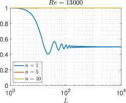
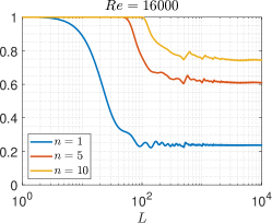
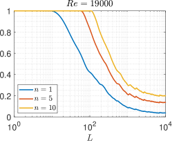
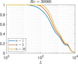
We apply the discrete-time RAGE theorem (Theorem B.22) to the mean-subtracted total kinetic energy as our observable . We use time-delay embedding as our projections corresponding to time delays. The values are computed by applying to the trajectory data of , which corresponds to a shift of the time series, and then using the Moore–Penrose inverse to apply the projection . The squared norm is computed using the ergodic theorem to approximate inner products. The results are shown in Figure 5 for various choices of . We observe the double limit at play. The results indicate that the spectrum is pure point for , mixed for and , but purely continuous for . This is consistent with the findings of [121, 46], where the authors computed spectral measures for this system. The figures in the main text illustrate the extraction of the pure point spectrum for . We used the method outlined in the proof of Theorem B.19. Specifically, the top panel shows the smoothed spectral measure with a second-order smoothing kernel (taken from [46]) and a smoothing parameter . The bottom panel displays the extracted pure point spectral measure, computed using the discrete-time RAGE theorem and a partition of the spectrum
References
- [1] Yann LeCun, Yoshua Bengio, and Geoffrey Hinton. Deep learning. Nature, 521(7553):436–444, May 2015.
- [2] John Jumper, Richard Evans, Alexander Pritzel, Tim Green, Michael Figurnov, Olaf Ronneberger, Kathryn Tunyasuvunakool, Russ Bates, Augustin Žídek, Anna Potapenko, et al. Highly accurate protein structure prediction with AlphaFold. Nature, 596(7873):583–589, July 2021.
- [3] Kaiming He, Xiangyu Zhang, Shaoqing Ren, and Jian Sun. Deep residual learning for image recognition. In 2016 IEEE Conference on Computer Vision and Pattern Recognition (CVPR). IEEE, June 2016.
- [4] Yonggang Yao, Qi Dong, Alexandra Brozena, Jian Luo, Jianwei Miao, Miaofang Chi, Chao Wang, Ioannis G. Kevrekidis, Zhiyong Jason Ren, Jeffrey Greeley, Guofeng Wang, Abraham Anapolsky, and Liangbing Hu. High-entropy nanoparticles: Synthesis-structure-property relationships and data-driven discovery. Science, 376(6589), April 2022.
- [5] Alex Zhavoronkov, Yan A. Ivanenkov, Alex Aliper, Mark S. Veselov, Vladimir A. Aladinskiy, Anastasiya V. Aladinskaya, Victor A. Terentiev, Daniil A. Polykovskiy, Maksim D. Kuznetsov, Arip Asadulaev, Yury Volkov, Artem Zholus, Rim R. Shayakhmetov, Alexander Zhebrak, Lidiya I. Minaeva, Bogdan A. Zagribelnyy, Lennart H. Lee, Richard Soll, David Madge, Li Xing, Tao Guo, and Alán Aspuru-Guzik. Deep learning enables rapid identification of potent DDR1 kinase inhibitors. Nature Biotechnology, 37(9):1038–1040, September 2019.
- [6] C. William Gear, James M. Hyman, Panagiotis G. Kevrekidid, Ioannis G. Kevrekidis, Olof Runborg, and Constantinos Theodoropoulos. Equation-free, coarse-grained multiscale computation: enabling microscopic simulators to perform system-level analysis. Communications in Mathematical Sciences, 1(4):715–762, 2003.
- [7] I. Mezić and A. Banaszuk. Comparison of systems with complex behavior. Physica D: Nonlinear Phenomena, 197(1-2):101–133, October 2004.
- [8] Igor Mezić. Spectral properties of dynamical systems, model reduction and decompositions. Nonlinear Dynamics, 41(1-3):309–325, August 2005.
- [9] R. R. Coifman, S. Lafon, A. B. Lee, M. Maggioni, B. Nadler, F. Warner, and S. W. Zucker. Geometric diffusions as a tool for harmonic analysis and structure definition of data: Diffusion maps. Proceedings of the National Academy of Sciences, 102(21):7426–7431, May 2005.
- [10] Ronald R. Coifman and Stéphane Lafon. Diffusion maps. Applied and Computational Harmonic Analysis, 21(1):5–30, July 2006.
- [11] Boaz Nadler, Stéphane Lafon, Ronald R. Coifman, and Ioannis G. Kevrekidis. Diffusion maps, spectral clustering and reaction coordinates of dynamical systems. Applied and Computational Harmonic Analysis, 21(1):113–127, July 2006.
- [12] Josh Bongard and Hod Lipson. Automated reverse engineering of nonlinear dynamical systems. Proceedings of the National Academy of Sciences, 104(24):9943–9948, June 2007.
- [13] Michael Schmidt and Hod Lipson. Distilling free-form natural laws from experimental data. Science, 324(5923):81–85, April 2009.
- [14] Amit Singer, Radek Erban, Ioannis G. Kevrekidis, and Ronald R. Coifman. Detecting intrinsic slow variables in stochastic dynamical systems by anisotropic diffusion maps. Proceedings of the National Academy of Sciences, 106(38):16090–16095, September 2009.
- [15] George Sugihara, Robert May, Hao Ye, Chih-hao Hsieh, Ethan Deyle, Michael Fogarty, and Stephan Munch. Detecting causality in complex ecosystems. Science, 338(6106):496–500, October 2012.
- [16] Steven L. Brunton, Joshua L. Proctor, and J. Nathan Kutz. Discovering governing equations from data by sparse identification of nonlinear dynamical systems. Proceedings of the National Academy of Sciences, 113(15):3932–3937, March 2016.
- [17] J. Nathan Kutz, Steven L. Brunton, Bingni W. Brunton, and Joshua L. Proctor. Dynamic Mode Decomposition: Data-Driven Modeling of Complex Systems. Society for Industrial and Applied Mathematics, November 2016.
- [18] Hassan Ismail Fawaz, Germain Forestier, Jonathan Weber, Lhassane Idoumghar, and Pierre-Alain Muller. Deep learning for time series classification: A review. Data mining and knowledge discovery, 33(4):917–963, March 2019.
- [19] Steven L. Brunton, Bernd R. Noack, and Petros Koumoutsakos. Machine learning for fluid mechanics. Annual Review of Fluid Mechanics, 52(1):477–508, January 2020.
- [20] Thomas M. Bury, R. I. Sujith, Induja Pavithran, Marten Scheffer, Timothy M. Lenton, Madhur Anand, and Chris T. Bauch. Deep learning for early warning signals of tipping points. Proceedings of the National Academy of Sciences, 118(39), September 2021.
- [21] Bernard O. Koopman. Hamiltonian systems and transformation in Hilbert space. Proceedings of the National Academy of Sciences, 17(5):315–318, May 1931.
- [22] Bernard O. Koopman and John von Neumann. Dynamical systems of continuous spectra. Proceedings of the National Academy of Sciences, 18(3):255–263, March 1932.
- [23] Marko Budišić, Ryan Mohr, and Igor Mezić. Applied Koopmanism. Chaos: An Interdisciplinary Journal of Nonlinear Science, 22(4):047510, December 2012.
- [24] Igor Mezić. Analysis of fluid flows via spectral properties of the Koopman operator. Annual Review of Fluid Mechanics, 45(1):357–378, January 2013.
- [25] Dimitrios Giannakis. Data-driven spectral decomposition and forecasting of ergodic dynamical systems. Applied and Computational Harmonic Analysis, 47(2):338–396, September 2019.
- [26] Samuel E. Otto and Clarence W. Rowley. Koopman operators for estimation and control of dynamical systems. Annual Review of Control, Robotics, and Autonomous Systems, 4(1):59–87, May 2021.
- [27] Steven L. Brunton, Marko Budišić, Eurika Kaiser, and J. Nathan Kutz. Modern Koopman theory for dynamical systems. SIAM Review, 64(2):229–340, May 2022.
- [28] Matthew J. Colbrook. The multiverse of dynamic mode decomposition algorithms, pages 127–230. Elsevier, 2024.
- [29] David A. Haggerty, Michael J. Banks, Ervin Kamenar, Alan B. Cao, Patrick C. Curtis, Igor Mezić, and Elliot W. Hawkes. Control of soft robots with inertial dynamics. Science Robotics, 8(81), August 2023.
- [30] Daniel Bruder, Brent Gillespie, C. David Remy, and Ram Vasudevan. Modeling and control of soft robots using the Koopman operator and model predictive control. In Robotics: Science and Systems XV, RSS2019. Robotics: Science and Systems Foundation, June 2019.
- [31] Xinyang Wang, Joanna Slawinska, and Dimitrios Giannakis. Extended-range statistical ENSO prediction through operator-theoretic techniques for nonlinear dynamics. Scientific Reports, 10(1), February 2020.
- [32] Gary Froyland, Dimitrios Giannakis, Benjamin R. Lintner, Maxwell Pike, and Joanna Slawinska. Spectral analysis of climate dynamics with operator-theoretic approaches. Nature Communications, 12(1), November 2021.
- [33] Antonio Orvieto, Samuel L. Smith, Albert Gu, Anushan Fernando, Caglar Gulcehre, Razvan Pascanu, and Soham De. Resurrecting recurrent neural networks for long sequences. In International Conference on Machine Learning, pages 26670–26698. PMLR, 2023.
- [34] Joshua L. Proctor and Philip A. Eckhoff. Discovering dynamic patterns from infectious disease data using dynamic mode decomposition. International Health, 7(2):139–145, February 2015.
- [35] Bingni W. Brunton, Lise A. Johnson, Jeffrey G. Ojemann, and J. Nathan Kutz. Extracting spatial-temporal coherent patterns in large-scale neural recordings using dynamic mode decomposition. Journal of Neuroscience Methods, 258:1–15, January 2016.
- [36] Bethany Lusch, J. Nathan Kutz, and Steven L. Brunton. Deep learning for universal linear embeddings of nonlinear dynamics. Nature Communications, 9(1):1–10, November 2018.
- [37] Peter J. Schmid. Dynamic mode decomposition of numerical and experimental data. Journal of Fluid Mechanics, 656:5–28, July 2010.
- [38] Clarence W. Rowley, Igor Mezić, Shervin Bagheri, Philipp Schlatter, and Dan S. Henningson. Spectral analysis of nonlinear flows. Journal of Fluid Mechanics, 641:115–127, November 2009.
- [39] Igor Mezić. On numerical approximations of the Koopman operator. Mathematics, 10(7):1180, April 2022.
- [40] Milan Korda, Mihai Putinar, and Igor Mezić. Data-driven spectral analysis of the Koopman operator. Applied and Computational Harmonic Analysis, 48(2):599–629, March 2020.
- [41] Dimitrios Giannakis, Amelia Henriksen, Joel A. Tropp, and Rachel Ward. Learning to forecast dynamical systems from streaming data. SIAM Journal on Applied Dynamical Systems, 22(2):527–558, May 2023.
- [42] Suddhasattwa Das, Dimitrios Giannakis, and Joanna Slawinska. Reproducing kernel Hilbert space compactification of unitary evolution groups. Applied and Computational Harmonic Analysis, 54:75–136, September 2021.
- [43] Dimitrios Giannakis and Claire Valva. Consistent spectral approximation of Koopman operators using resolvent compactification. Nonlinearity, 37(7):075021, June 2024.
- [44] Matthew J. Colbrook and Alex Townsend. Rigorous data-driven computation of spectral properties of Koopman operators for dynamical systems. Communications on Pure and Applied Mathematics, 77(1):221–283, July 2023.
- [45] Matthew J. Colbrook. The mpEDMD algorithm for data-driven computations of measure-preserving dynamical systems. SIAM Journal on Numerical Analysis, 61(3):1585–1608, June 2023.
- [46] Matthew J. Colbrook, Catherine Drysdale, and Andrew Horning. Rigged Dynamic Mode Decomposition: Data-driven generalized eigenfunction decompositions for Koopman operators. arXiv preprint arXiv:2405.00782, 2024.
- [47] Matthew O. Williams, Ioannis G. Kevrekidis, and Clarence W. Rowley. A data–driven approximation of the Koopman operator: Extending dynamic mode decomposition. Journal of Nonlinear Science, 25(6):1307–1346, June 2015.
- [48] Milan Korda and Igor Mezić. On convergence of extended dynamic mode decomposition to the Koopman operator. Journal of Nonlinear Science, 28(2):687–710, November 2018.
- [49] Anders Hansen. On the solvability complexity index, the -pseudospectrum and approximations of spectra of operators. Journal of the American Mathematical Society, 24(1):81–124, July 2011.
- [50] Jonathan Ben-Artzi, Matthew J. Colbrook, Anders C. Hansen, Olavi Nevanlinna, and Markus Seidel. Computing spectra - On the solvability complexity index hierarchy and towers of algorithms. arXiv, 2020.
- [51] Matthew J. Colbrook. The foundations of infinite-dimensional spectral computations. PhD thesis, University of Cambridge, 2020.
- [52] Steve Smale. On the efficiency of algorithms of analysis. Bulletin of the American Mathematical Society, 13(2):87–122, 1985.
- [53] Curt McMullen. Families of rational maps and iterative root-finding algorithms. Annals of Mathematics, 125(3):467–493, 1987.
- [54] Curt McMullen. Braiding of the attractor and the failure of iterative algorithms. Inventiones Mathematicae, 91(2):259–272, 1988.
- [55] Peter Doyle and Curt McMullen. Solving the quintic by iteration. Acta Mathematica, 163(1):151–180, 1989.
- [56] Steve Smale. The work of Curtis T. McMullen. In Proceedings of the International Congress of Mathematicians 1998, pages 127–132. EMS Press, 1998.
- [57] Gabor Szegő. Beiträge zur Theorie der Toeplitzschen Formen. Mathematische Zeitschrift, 6(3-4):167–202, 1920.
- [58] Julian Schwinger. The special canonical group. Proceedings of the National Academy of Sciences, 46(10):1401–1415, 1960.
- [59] Igor Mezić. On the geometrical and statistical properties of dynamical systems: Theory and applications. PhD thesis, 1994.
- [60] Ricardo Mañé. Ergodic Theory and Differentiable Dynamics. Number v.8. Springer Berlin Heidelberg, Berlin, Heidelberg, 1987. Description based on publisher supplied metadata and other sources.
- [61] I. Mezić. Koopman operator, geometry, and learning of dynamical systems. Notices of the American Mathematical Society, 68(07):1, August 2021.
- [62] Alexandre Mauroy and Igor Mezić. Global stability analysis using the eigenfunctions of the Koopman operator. IEEE Transactions on Automatic Control, 61(11):3356–3369, November 2016.
- [63] Igor Mezić. On applications of the spectral theory of the Koopman operator in dynamical systems and control theory. In 2015 54th IEEE Conference on Decision and Control (CDC), pages 7034–7041. IEEE, December 2015.
- [64] Alexandre Mauroy, Igor Mezić, and Jeff Moehlis. Isostables, isochrons, and Koopman spectrum for the action–angle representation of stable fixed point dynamics. Physica D: Nonlinear Phenomena, 261:19–30, October 2013.
- [65] Jiajie Chen and Thomas Y. Hou. Stable nearly self-similar blowup of the 2D Boussinesq and 3D Euler equations with smooth data II: Rigorous numerics. arXiv:2305.05660, 2023.
- [66] J. Cepelewicz. Deep learning poised to ”blow up” famed fluid equations, Quanta, April 12, 2022.
- [67] Michael I. Gil’. Operator Functions and Localization of Spectra. Springer Berlin Heidelberg, 2003.
- [68] Peter Henrici. Bounds for iterates, inverses, spectral variation and fields of values of non-normal matrices. Numerische Mathematik, 4(1):24–40, December 1962.
- [69] Zlatko Drmač and Igor Mezić. A data driven Koopman-Schur decomposition for computational analysis of nonlinear dynamics. arXiv preprint arXiv:2312.15837, 2023.
- [70] Igor Mezić. Spectrum of the Koopman operator, spectral expansions in functional spaces, and state-space geometry. Journal of Nonlinear Science, 30(5):2091–2145, December 2020.
- [71] Russel E. Caflisch. Monte Carlo and quasi-Monte Carlo methods. Acta Numerica, 7:1–49, January 1998.
- [72] Alan M. Turing. On computable numbers, with an application to the Entscheidungsproblem. Proceedings of the London Mathematical Society, s2-42(1):230–265, 1937.
- [73] Lenore Blum, Felipe Cucker, Michael Shub, and Steve Smale. Complexity and Real Computation. Springer eBook Collection. Springer, New York, NY, 1998.
- [74] Ricardo Mañé. Ergodic theory and differentiable dynamics, volume 8. Springer Science & Business Media, 2012.
- [75] Michael Dellnitz and Oliver Junge. On the approximation of complicated dynamical behavior. SIAM Journal on Numerical Analysis, 36(2):491–515, January 1999.
- [76] Gerhard Keller and Carlangelo Liverani. Stability of the spectrum for transfer operators. Annali della Scuola Normale Superiore di Pisa-Classe di Scienze, 28(1):141–152, 1999.
- [77] Gary Froyland. On Ulam approximation of the isolated spectrum and eigenfunctions of hyperbolic maps. Discrete and Continuous Dynamical Systems, 17(3):671–689, 2007.
- [78] Gary Froyland, Cecilia González-Tokman, and Anthony Quas. Detecting isolated spectrum of transfer and Koopman operators with Fourier analytic tools. Journal of Computational Dynamics, 1(2):249–278, 2014.
- [79] Harry Crimmins and Gary Froyland. Fourier approximation of the statistical properties of Anosov maps on tori. Nonlinearity, 33(11):6244–6296, October 2020.
- [80] Michael Blank, Gerhard Keller, and Carlangelo Liverani. Ruelle–Perron–Frobenius spectrum for Anosov maps. Nonlinearity, 15(6):1905–1973, September 2002.
- [81] Stefan Klus, Feliks Nüske, Péter Koltai, Hao Wu, Ioannis Kevrekidis, Christof Schütte, and Frank Noé. Data-driven model reduction and transfer operator approximation. Journal of Nonlinear Science, 28(3):985–1010, January 2018.
- [82] Sebastian Peitz and Stefan Klus. Koopman operator-based model reduction for switched-system control of PDEs. Automatica, 106:184–191, August 2019.
- [83] Alexander Grigoryevich Kachurovskii. The rate of convergence in ergodic theorems. Russian Mathematical Surveys, 51(4):653–703, August 1996.
- [84] Matthew J. Colbrook. Computing spectral measures and spectral types. Communications in Mathematical Physics, 384(1):433–501, April 2021.
- [85] Hassan Arbabi and Igor Mezić. Ergodic theory, dynamic mode decomposition, and computation of spectral properties of the Koopman operator. SIAM Journal on Applied Dynamical Systems, 16(4):2096–2126, January 2017.
- [86] Nithin Govindarajan, Ryan Mohr, Shivkumar Chandrasekaran, and Igor Mezić. On the approximation of Koopman spectra for measure preserving transformations. SIAM Journal on Applied Dynamical Systems, 18(3):1454–1497, January 2019.
- [87] Nicolas Boullé and Matthew J. Colbrook. Multiplicative dynamic mode decomposition. arXiv preprint arXiv:2405.05334, 2024.
- [88] Stefan Klus, Feliks Nüske, Sebastian Peitz, Jan-Hendrik Niemann, Cecilia Clementi, and Christof Schütte. Data-driven approximation of the Koopman generator: Model reduction, system identification, and control. Physica D: Nonlinear Phenomena, 406:132416, May 2020.
- [89] Nicolas Boullé and Matthew J. Colbrook. On the convergence of Hermitian dynamic mode decomposition. arXiv preprint arXiv:2401.03192, 2024.
- [90] Tyrus Berry, Dimitrios Giannakis, and John Harlim. Nonparametric forecasting of low-dimensional dynamical systems. Physical Review E, 91(3):032915, March 2015.
- [91] Jake Fillman and Darren C. Ong. Purely singular continuous spectrum for limit-periodic CMV operators with applications to quantum walks. Journal of Functional Analysis, 272(12):5107–5143, June 2017.
- [92] Nicolas Boullé, Diana Halikias, and Alex Townsend. Elliptic PDE learning is provably data-efficient. Proceedings of the National Academy of Sciences, 120(39), September 2023.
- [93] Stefano Luzzatto, Ian Melbourne, and Frederic Paccaut. The Lorenz attractor is mixing. Communications in Mathematical Physics, 260(2):393–401, August 2005.
- [94] Tanja Eisner, Bálint Farkas, Markus Haase, and Rainer Nagel. Operator theoretic aspects of ergodic theory, volume 272. Springer International Publishing, 2015.
- [95] Matthew J. Colbrook. Computing semigroups with error control. SIAM Journal on Numerical Analysis, 60(1):396–422, 2022.
- [96] Simon Becker and Anders Hansen. Computing solutions of schr” odinger equations on unbounded domains-on the brink of numerical algorithms. arXiv preprint arXiv:2010.16347, 2020.
- [97] Matthew J. Colbrook, Vegard Antun, and Anders C. Hansen. The difficulty of computing stable and accurate neural networks: On the barriers of deep learning and Smale’s 18th problem. Proceedings of the National Academy of Sciences, 119(12):e2107151119, 2022.
- [98] A. Bastounis, A. C. Hansen, and V. Vlačić. The extended Smale’s 9th problem – On computational barriers and paradoxes in estimation, regularisation, computer-assisted proofs and learning. arXiv preprint arXiv:2110.15734, 2021.
- [99] Matthew J. Colbrook, Bogdan Roman, and Anders C. Hansen. How to compute spectra with error control. Physical Review Letters, 122(25):250201, 2019.
- [100] Matthew J. Colbrook and Anders C. Hansen. The foundations of spectral computations via the solvability complexity index hierarchy. Journal of the European Mathematical Society, 25(12):4639–4728, November 2022.
- [101] Sanjeev Arora and Boaz Barak. Computational complexity: a modern approach. Cambridge University Press, 2009.
- [102] Isaac P. Cornfeld, Sergej V. Fomin, and Yakov Grigorevich Sinai. Ergodic theory, volume 245. Springer Science & Business Media, 2012.
- [103] Peter Walters. An introduction to ergodic theory, volume 79 of Graduate texts in mathematics. Springer, New York, 1. softcover printing edition, 2000.
- [104] Igor Mezić and Stephen Wiggins. A method for visualization of invariant sets of dynamical systems based on the ergodic partition. Chaos: An Interdisciplinary Journal of Nonlinear Science, 9(1):213–218, 1999.
- [105] Donald L. Cohn. Measure theory, volume 5. Springer, 2013.
- [106] Gerald B. Folland. Real Analysis: Modern Techniques and their Applications, volume 40 of Pure and applied mathematics. Wiley, New York, 2. ed. edition, 1999. ”A Wiley-Interscience publication.” - Includes bibliographical references and index.
- [107] Béla Sz Nagy, Ciprian Foias, Hari Bercovici, and László Kérchy. Harmonic analysis of operators on Hilbert space. Springer New York, 2010.
- [108] Matthew J. Colbrook, Lorna J. Ayton, and Máté Szőke. Residual dynamic mode decomposition: Robust and verified Koopmanism. Journal of Fluid Mechanics, 955:A21, January 2023.
- [109] A. B. Brown and M. Halperin. On certain area-preserving maps. Annals of Mathematics, pages 833–837, 1935.
- [110] Gilbert Levitt. Feuilletages des surfaces. In Annales de l’institut Fourier, volume 32, pages 179–217, 1982.
- [111] Michael Aizenman and Simone Warzel. Random Operators, volume 168 of Graduate Studies in Mathematics. American Mathematical Society, 2015.
- [112] David Ruelle. A remark on bound states in potential-scattering theory. Il Nuovo Cimento A, 61(4):655–662, 1969.
- [113] W. O. Amrein and V. Georgescu. On the characterization of bound states and scattering states in quantum mechanics. Helvetica Physica Acta. Physica Theoretica. Societatis Physicae Helveticae Commentaria Publica, 46(5):635–658, 1973.
- [114] Volker Enss. Asymptotic completeness for quantum mechanical potential scattering. I. Short range potentials. Communications in Mathematical Physics, 61(3):285–291, 1978.
- [115] Matthew J. Colbrook. On the computation of geometric features of spectra of linear operators on Hilbert spaces. Foundations of Computational Mathematics, 24(3):723–804, December 2022.
- [116] Jie Shen. Hopf bifurcation of the unsteady regularized driven cavity flow. Journal of Computational Physics, 95(1):228–245, July 1991.
- [117] Maciej J. Balajewicz, Earl H. Dowell, and Bernd R. Noack. Low-dimensional modelling of high-Reynolds-number shear flows incorporating constraints from the Navier–Stokes equation. Journal of Fluid Mechanics, 729:285–308, July 2013.
- [118] Olivier Botella. On the solution of the Navier-Stokes equations using Chebyshev projection schemes with third-order accuracy in time. Computers & Fluids, 26(2):107–116, February 1997.
- [119] Roger Temam. Infinite-dimensional dynamical systems in mechanics and physics, volume 68 of Applied Mathematical Sciences. Springer-Verlag, New York, 2012.
- [120] Lloyd N. Trefethen. Spectral methods in MATLAB. Society for Industrial and Applied Mathematics, January 2000.
- [121] Hassan Arbabi and Igor Mezić. Study of dynamics in post-transient flows using Koopman mode decomposition. Physical Review Fluids, 2(12):124402, December 2017.