Decoupling Local Primordial non-Gaussianity from Relativistic Effects in the Galaxy Bispectrum

Abstract

Upcoming galaxy surveys aim to map the Universe with unprecedented precision, depth and sky coverage. The galaxy bispectrum is a prime source of information as it allows us to probe primordial non-Gaussianity (PNG), a key factor in differentiating various models of inflation. On the scales where local PNG is strongest, Doppler and other relativistic effects become important and need to be included. We investigate the detectability of relativistic and local PNG contributions in the galaxy bispectrum. We compute the signal-to-noise ratio for the detection of the bispectrum including such effects. Furthermore, we perform information matrix forecasts on the local PNG parameter $f_{\rm NL}$ and on the parametrised amplitudes of the relativistic corrections. Finally, we quantify the bias on the measurement of $f_{\rm NL}$ that arises from neglecting relativistic effects. Our results show that detections of both first- and second-order relativistic effects are promising with forthcoming spectroscopic survey specifications – and are largely unaffected by the uncertainty in $f_{\rm NL}$. Conversely, we show for the first time that neglecting relativistic corrections in the galaxy bispectrum can lead to $>\!1.5\sigma(f_{\rm NL})$ shift on the detected value of $f_{\rm NL}$, highlighting the importance of including relativistic effects in our modelling.

1 Introduction

Advancements in observational cosmology, as well as sophisticated theoretical cosmological and statistical modeling, have propelled our understanding of the large-scale structure of the universe to new heights. With the wide variety of probes of large-scale structure, tracers of the underlying matter distribution, and their corresponding observational techniques and missions, the promise of new physics is littered with nuance which requires detailed attention to the contributions that may distort, enhance, or cloud our visual description of the distribution of these structures.

Galaxy surveys have long been an indispensable probe of large-scale structure. We can infer the underlying physics that governs the evolution of matter perturbations by observing the fluctuations of galaxy distributions at different scales and redshifts, and therefore test theories of gravity. The anticipated measurements from current and future surveys such as the Dark Energy Spectroscopic Instrument (DESI) [1, 2], the Euclid satellite mission [3, 4], the Nancy Grace Roman Space Telescope [5, 6] and MegaMapper [7], have or will provide information on ultra-large scales i.e from beyond the matter-radiation equality scale. At these scales primordial non-Gaussianity can be probed. It is also at this scale that effects from general relativity have the most impact on our measurements. This is the key motivation of this paper, quantifying how corrections to the galaxy number density which appear due to general relativity, specifically those derived from observing on our past lightcone, effect measurements of PNG. We explore this through the galaxy bispectrum, the fourier transform of the 3 point correlation function of galaxy density contrasts, which is only non-zero in the presence of non-Gaussianity. Doppler shifts induced by the peculiar velocities of galaxies, gravitational lensing effects, and other relativistic corrections alter the clustering patterns of galaxies, imprinting distinct signatures on the bispectrum which mimic that of PNG [8, 9, 10, 11]. Therefore, understanding and accurately modeling these relativistic effects are imperative for extracting robust cosmological information from galaxy surveys.

The $f_{\mathrm{NL}}$ parameter, which we use to quantify so-called local Primordial non-Gaussianity (PNG), provides an excellent way to test theories of inflation, many of which depend heavily on constraints to this. PNG arises from departures of the primordial density fluctuations from a purely Gaussian distribution, a characteristic feature predicted by many inflationary models. Local PNG affects the bispectrum on ultra-large scales, which is also where the relativistic effects are strongest. Therefore, in a Newtonian bispectrum analysis, the unaccounted for relativistic contaminations would induce biases to the primordial signal, meaning a Gaussian primordial universe could be incorrectly found to be non-Gaussian [10, 11, 8, 12, 9, 13, 14]. As a community, we seem to have reached a maximum in how much we can constrain $f_{\mathrm{NL}}$ using measurements from the CMB, obtaining a measurement of $f_{\mathrm{NL}}=-0.9\pm 5.1$ from Planck 2018 [15]. In order to improve our constraints, we can fine-tune our modeling of relativistic corrections to our observables.

The galaxy power spectrum has been extensively studied and used to obtain impressive constraints on cosmological parameters. The dominant perturbation effect on sub-Hubble scales is from redshift-space distortions (RSD) [16], which constitute the standard Newtonian approximation to projection effects. The inclusion of relativistic corrections to the galaxy density contrast at linear order [17, 18, 19, 10, 20] has, in turn, provided further insights. Many studies have been done on the possibility of constraining the local PNG parameter $f_{\mathrm{NL}}$ using the relativistic galaxy power spectrum for future galaxy and intensity mapping surveys, which avoids the Gaussian bias typical in the Newtonian analysis [21, 22, 10, 11, 8, 23, 24, 25, 26, 27, 28, 29, 30, 31, 32, 33, 34, 35, 36]. PNG in the galaxy bispectrum has been extensively investigated in the Newtonian approximation [37, 38, 39, 40, 41, 42, 43, 44, 45, 46, 47, 48, 49, 50, 51, 52, 53, 54]. In a paper by Tellarini et al [39] it was shown that constraints on $f_{\mathrm{NL}}$ can be obtained from LSS which are competitive to that of Planck with forcasts on the Newtonian tree level bispectrum (including RSD to second order) using survey specifications from BOSS [55], eBOSS [56], Euclid [57] and DESI (LRGs, ELGs and QSOs) [58].

To compute the relativistic galaxy bispectrum, we require the observed galaxy number density contrast to second order in perturbation theory, which has been done independently several times [59, 60, 61, 62, 63]. At second order, the relativistic corrections are much more elaborate than those at first order because they involve quadratic couplings of first-order terms, introduce new terms such as the transverse peculiar velocity, lensing deflection angle and lensing sheer, include second-order relativistic correction to the galaxy bias, and require second-order gauge corrections to the second-order number density.

The relativistic corrections to the second order galaxy bias model have been calculated with Gaussian initial conditions [64] and in the presence of local PNG [65]. There are no such corrections to the first order galaxy bias, thus, the tree-level power spectrum does not contain a relativistic correction to the bias model, but the tree-level bispectrum does. Furthermore, the local PNG signal in the tree-level galaxy power spectrum is sourced only by scale-dependent bias [66, 67], since there is no PNG signal in the primordial matter power spectrum at tree level. However, the local PNG in the galaxy bispectrum is sourced by scale-dependent bias, primordial matter bispectrum, and RSD at second order [39]. Notably, second-order relativistic corrections to RSD lead to new local PNG effects in the bispectrum. These effects arise from the coupling of first-order scale-dependent bias to first-order relativistic projection effects and the linearly evolved PNG in second-order velocity and metric potentials, which are absent in the standard Newtonian analysis.

In this paper, we compare current and future survey specifications by forecasting the amplitude of GR contributions, isolating the first order and second order corrections. We then perform an information matrix analysis to obtain the marginal errors on the $f_{\mathrm{NL}}$ parameter for local PNG and on each GR amplitude. We emphasise the importance of including contributions by calculating the $f_{\mathrm{NL}}$ bias, inherent in the Newtonian regime. Our work follows a series of papers which explore a particular model of the galaxy bispectrum [9] which includes non-integrated local lightcone projection effects [68, 69, 70, 71, 13, 72, 73, 74]. We take exactly the model of the galaxy bispectrum from Maartens et al [75] in which the authors extend the previous list of works to incorporate local PNG into the relativistic bispectrum. This involves applying the recent results of [65, 64] on relativistic corrections to the second-order galaxy bias model. In line with the literature, we use the Fourier bispectrum, adopting a plane-parallel approximation.

2 The galaxy bispectrum

We begin by outlining the model of the galaxy bispectrum for which we implement our analysis. The full description of this model can be found in [75], which calculates the relativistic contributions to the galaxy bispectrum in the presence of local PNG by extending the derivation of the relativistic galaxy overdensity [9, 13, 72, 73, 68], neglecting integrated effects. Here we only present the key details relevant to our analysis. At tree level, the observed galaxy bispectrum is defined by

$$2\,\left<\varDelta_{\rm g}(\bm{k}_{1})\,\varDelta_{\rm g}(\bm{k}_{2})\,\varDelta_{\rm g}^{(2)}(\bm{k}_{3})\right>+2\,\mathrm{cp}=(2\pi)^{3}\,B_{\rm g}(\bm{k}_{1},\bm{k}_{2},\bm{k}_{3})\,\delta^{D}(\bm{k}_{1}+\bm{k}_{2}\,+\bm{k}_{2})\quad,$$ (2.1)

where we use the convention that the observed density contrast is $\varDelta_{\rm g}+\varDelta_{\rm g}^{(2)}/2$ and is related at first order to the number density contrast at the source $\delta_{\rm g}$ by

$$\varDelta_{\rm g}=\delta_{\rm g}+\mathrm{RSD}+\text{relativistic effects}+\text{local PNG contributions}$$ (2.2)

It can then be written in terms of first- and second-order Fourier kernels as

$$B_{\rm g}(\bm{k}_{1},\bm{k}_{2},\bm{k}_{3})=\mathcal{K}^{(1)}(\bm{k}_{1})\,\mathcal{K}^{(1)}(\bm{k}_{2})\,\mathcal{K}^{(2)}(\bm{k}_{1},\bm{k}_{2},\bm{k}_{3})\,P(\bm{k}_{1})\,P(\bm{k}_{2})+2\,\mathrm{cp}$$ (2.3)

where $P$ is the linear matter power spectrum and the kernels $\mathcal{K}^{(i)}$ are a summation of Newtonian, relativistic and local PNG contributions, i.e. $\mathcal{K}^{(i)}=\mathcal{K}^{(i)}_{\mathrm{N}}+\mathcal{K}^{(i)}_{\mathrm{GR}}+\mathcal{K}^{(i)}_{\mathrm{PNG}}$, for $i=1,2$. In writing the galaxy bispectrum this way, it is simple to isolate the effects we want to study. The Newtonian bispectrum is simply:

$$B_{\rm gN}(\bm{k}_{1},\bm{k}_{2},\bm{k}_{3})=\mathcal{K}_{\rm N}^{(1)}(\bm{k}_{1})\,\mathcal{K}_{\rm N}^{(1)}(\bm{k}_{2})\,\mathcal{K}_{\rm N}^{(2)}(\bm{k}_{1},\bm{k}_{2},\bm{k}_{3})\,P(\bm{k}_{1})\,P(\bm{k}_{2})+2\,\mathrm{cp}$$ (2.4)

with

$$\mathcal{K}_{\mathrm{N}}^{(1)}(\bm{k}_{a}) =b_{10}+f\,\mu_{a}^{2}\,$$ (2.5)

$$\mathcal{K}_{\mathrm{N}}^{(2)}(\bm{k}_{1},\bm{k}_{2},\bm{k}_{3}) =b_{10}\,F_{2}(\bm{k}_{1},\bm{k}_{2})+b_{20}+f\,\mu_{3}^{2}\,G_{2}(\bm{k}_{1},\bm{k}_{2})+b_{s}\,S_{2}\,(\bm{k}_{1},\bm{k}_{2})$$

$$\quad+b_{10}\,f\,\left(\mu_{1}\,k_{1}+\mu_{2}\,k_{2}\right)\,\left(\frac{\mu_{1}}{k_{1}}+\frac{\mu_{2}}{k_{2}}\right)+f^{2}\,\frac{\mu_{1}\,\mu_{2}}{k_{1}\,k_{2}}\left(\mu_{1}\,k_{1}+\mu_{2}\,k_{2}\right)^{2}$$ (2.6)

where $\mu_{a}=\hat{\bm{k}}_{a}\cdot\bm{n}$ and for the growth factor $D$ and scale factor $a$, $f=\mathrm{d}\ln D/\mathrm{d}\ln a$ is the linear matter growth rate. The kernels $F_{2}$ (mode-coupling part of the matter density contrast), $G_{2}$ (mode-coupling part of the matter velocity), and $S_{2}$ (tidal bias) are given in Section A.1, with the linear and quadratic Gaussian clustering biases $b_{10}$ and $b_{20}$ given in Section A.2. The second line of Eq. 2.6 is the second-order RSD term. The contributions from local PNG or general relativity are omitted, apart from RSD – which is such an essential effect to account for that it is now generally included in the basic Newtonian framework.

The local general relativistic kernels at all orders of $\mathcal{H}/k$ are

$$\mathcal{K}_{\mathrm{GR}}^{(1)}(\bm{k}_{a}) =\mathrm{i}\,\mu_{a}\,\frac{\gamma_{1}}{k_{a}}+\frac{\gamma_{2}}{k_{a}^{2}}\;,$$ (2.7)

$$\mathcal{K}_{\mathrm{GR}}^{(2)}(\bm{k}_{1},\bm{k}_{2},\bm{k}_{3}) =\frac{1}{k_{1}^{2}\,k_{2}^{2}}\bigg{\{}\,\beta_{1}+E_{2}(\bm{k}_{1},\bm{k}_{2},\bm{k}_{3})\,\beta_{2}\,$$

$$\quad+\mathrm{i}\,\Big{[}\big{(}\mu_{1}\,k_{1}+\mu_{2}\,k_{2}\big{)}\,\beta_{3}+\mu_{3}\,k_{3}\,\big{\{}\beta_{4}+E_{2}(\bm{k}_{1},\bm{k}_{2},\bm{k}_{3})\,\beta_{5}\big{\}}\Big{]}$$

$$\quad+\frac{k_{1}^{2}\,k_{2}^{2}}{k_{3}^{2}}\,\Big{[}F_{2}(\bm{k}_{1},\bm{k}_{2})\,\beta_{6}+G_{2}(\bm{k}_{1},\bm{k}_{2})\,\beta_{7}\Big{]}+\left(\mu_{1}\,k_{1}\mu_{2}\,k_{2}\right)\,\beta_{8}$$

$$\quad+\mu_{3}^{2}\,k_{3}^{2}\,\Big{[}\beta_{9}+E_{2}(\bm{k}_{1},\bm{k}_{2},\bm{k}_{3})\,\beta_{10}\Big{]}+\left(\bm{k}_{1}\cdot\bm{k}_{2}\right)\,\beta_{11}$$

$$\quad+\left(k_{1}^{2}+k_{2}^{2}\right)\,\beta_{12}+\left(\mu_{1}^{2}\,k_{1}^{2}+\mu_{2}^{2}\,k_{2}^{2}\right)\,\beta_{13}$$

$$\quad+\mathrm{i}\,\Big{[}\left(\mu_{1}\,k_{1}^{3}+\mu_{2}\,k_{2}^{3}\right)\,\beta_{14}+\left(\mu_{1}\,k_{1}+\mu_{2}\,k_{2}\right)\left(\bm{k}_{1}\cdot\bm{k}_{2}\right)\,\beta_{15}$$

$$\quad+k_{1}\,k_{2}\,\left(\mu_{1}\,k_{2}+\mu_{2}\,k_{1}\right)\,\beta_{16}+\left(\mu_{1}^{3}\,k_{1}^{3}+\mu_{2}^{3}\,k_{2}^{3}\right)\,\beta_{17}$$

$$\quad+\mu_{1}\,\mu_{2}\,k_{1}\,k_{2}\,\left(\mu_{1}\,k_{1}+\mu_{2}\,k_{2}\right)\,\beta_{18}+\mu_{3}\,\frac{k_{1}^{2}\,k_{2}^{2}}{k_{3}}\,G_{2}(\bm{k}_{1},\bm{k}_{2})\,\beta_{19}\Big{]}\bigg{\}}\;,$$ (2.8)

where $E_{2}$ is given in Section A.1 and the time-dependent beta functions $\beta_{I}$ are given in Appendix D. We also have,

$$\frac{\gamma_{1}}{\mathcal{H}} =f\,\left[\mathcal{E}-2\,\mathcal{Q}-\frac{2\,(1-\mathcal{Q})}{\chi\mathcal{H}}-\frac{\mathcal{H}^{\prime}}{\mathcal{H}^{2}}\right]\;,$$ (2.9)

$$\frac{\gamma_{2}}{\mathcal{H}^{2}} =f\,\left(3-\mathcal{E}\,\right)+\frac{3}{2}\,\varOmega_{\rm m}\,\left[2+\mathcal{E}-f-4\,\mathcal{Q}-\frac{2\,(1-\mathcal{Q})}{\chi\,\mathcal{H}}-\frac{\mathcal{H}^{\prime}}{\mathcal{H}^{2}}\right]\;,$$ (2.10)

where $\varOmega_{\rm m}(z)=\varOmega_{{\rm m}0}\,H_{0}^{2}\,(1+z)/\mathcal{H}(z)^{2}$ is the matter density at redshift $z$ and $\mathcal{H}$ is the conformal Hubble parameter. Eq. 2.10 introduces some key aspects of a relativistic analysis, the magnification bias $\mathcal{Q}$ and the evolution bias $\mathcal{E}$. These arise due to dependencies on the survey luminosity function in detecting the comoving galaxy number density (see Appendix B for an example of how these biases are calculated).

Finally, the local PNG kernels are

$$\mathcal{K}_{\mathrm{nG}}^{(1)}(\bm{k}_{a}) =\frac{b_{01}}{\mathcal{M}_{a}}\quad\mbox{where}~{}~{}\mathcal{M}_{a}\equiv\mathcal{M}(\bm{k}_{a})=\frac{2\,D}{3\,D_{\rm in}\,\varOmega_{m}\,\mathcal{H}^{2}}\,T(k_{a})\,k_{a}^{2}\,,$$ (2.11)

$$\mathcal{K}_{\mathrm{nG}}^{(2)}(\bm{k}_{1},\bm{k}_{2},\bm{k}_{3}) =2\,f_{\mathrm{NL}}\,\left(b_{10}+f\,\mu_{3}^{2}\right)\,\frac{\mathcal{M}_{3}}{\mathcal{M}_{1}\,\mathcal{M}_{2}}+f\,b_{01}\,\left(\mu_{1}\,k_{1}+\mu_{2}\,k_{2}\right)\,\left(\frac{\mu_{1}}{k_{1}\,\mathcal{M}_{2}}+\frac{\mu_{2}}{k_{2}\,\mathcal{M}_{1}}\right)$$

$$\quad+b_{\rm N}\,N_{2}(\bm{k}_{1},\bm{k}_{2})+\frac{b_{11}}{2}\,\left(\frac{1}{\mathcal{M}_{1}}+\frac{1}{\mathcal{M}_{2}}\right)+\frac{b_{02}}{\mathcal{M}_{1}\mathcal{M}_{2}}$$

$$\quad+\frac{\mathcal{M}_{3}}{\mathcal{M}_{1}\,\mathcal{M}_{2}}\,\left(\frac{\varUpsilon_{1}}{k_{3}^{2}}+\mathrm{i}\,\frac{\mu_{3}}{k_{3}}\,\varUpsilon_{2}\right)+\varUpsilon_{3}\,\left(\frac{1}{k_{1}^{2}\,\mathcal{M}_{2}}+\frac{1}{k_{2}^{2}\,\mathcal{M}_{1}}\right)$$

$$\quad+\mathrm{i}\,\left[\varUpsilon_{4}\,\left(\frac{\mu_{1}\,k_{1}}{k_{2}^{2}\,\mathcal{M}_{1}}+\frac{\mu_{2}\,k_{2}}{k_{1}^{2}\,\mathcal{M}_{2}}\right)+\varUpsilon_{5}\,\left(\frac{\mu_{1}}{k_{1}\mathcal{M}_{2}}+\frac{\mu_{2}}{k_{2}\,\mathcal{M}_{1}}\right)\right]\;.$$ (2.12)

The transfer function $T(k_{a})$ relates the Gaussian potential to the linear primordial potential i.e $\varphi_{\text{in }}(\bm{k})=T(k)\,\varphi_{\mathrm{p}}(\bm{k})\quad$ for $\quad a_{\mathrm{p}}\ll a_{\mathrm{eq}}\ll a_{\mathrm{in}}$. The local PNG Fourier kernel, $N_{2}$, is given in Section A.1, the time-dependent, $\varUpsilon_{I}$, are given in Appendix E and the local PNG biases, $b_{01}$, $b_{\rm N}$, $b_{11}$ and $b_{02}$, are given in Section A.3. It is important to note that the last two lines of Eq. 2.12, containing the $\varUpsilon_{I}$ functions, arise from relativistic projection terms in $\varDelta_{g}^{(2)}$ and thus count as both relativistic corrections and local PNG contributions. Therefore, the total galaxy bispectrum is made up of the Newtoninan galaxy bispectrum, the purely relativistic corrections, purely local PNG corrections, plus the cross terms. The Newtonian and RSD parts are real and have no overall $k$ scaling, while PNG contributions are real and contribute to even powers of ${\cal H}/k$. Relativistic Doppler contributions also contribute at odd powers of $H/k$. These odd powers are imaginary and contribute to the odd multipoles in general. This model is the basis for our forecasting analysis. We expect there to be a degeneracy between PNG and relativistic contributions that scale as $({\cal H}/k)^{2}$, and our aim is to see if we can disentangle these. Because the relativistic parts also contribute at other powers of ${\cal H}/k$, we anticipate that we can.

3 Methodology

In this section, we outline the formalism employed for the signal-to-noise ratio (SNR), Fisher information matrix and parameter estimation bias. We justify our choice of parameter space and survey specifications for optimization of these analyses.

3.1 Signal-to-noise ratio

We extend the ${\rm SNR}$ analysis of [68] to our model with all orders of $H/k$ and including local PNG. Under the assumption of Gaussian statistics for the bispectrum and a diagonal covariance matrix, the ${\rm SNR}$ is given by

$${\rm SNR}^{2}(z)=\sum_{k_{a},\mu_{1},\varphi}\frac{1}{\operatorname{Var}\left[B_{g}\left(z,k_{a},\mu_{1},\varphi\right)\right]}B(z,k_{a},\mu_{1},\varphi)B^{\ast}(z,k_{a},\mu_{1},\varphi)D_{B}^{2}(z,k_{a},\mu_{1},\varphi)\;,$$ (3.1)

with the (Gaussian) variance reading

$$\operatorname{Var}\left[B_{g}\left(z,k_{a},\mu_{1},\varphi\right)\right]=s_{B}\,\frac{\pi\,k_{\rm f}^{3}(z)}{k_{1}\,k_{2}\,k_{3}\,\varDelta k^{3}}\frac{N_{\mu_{1}}}{\varDelta\mu_{1}}\,\frac{N_{\varphi}}{\varDelta\varphi}\,\tilde{P}_{\rm g\mathrm{N}}\left(z,k_{1},\mu_{1}\right)\,\tilde{P}_{\rm g\mathrm{N}}\left(z,k_{2},\mu_{2}\right)\,\tilde{P}_{\rm g\mathrm{N}}\left(z,k_{3},\mu_{3}\right).$$ (3.2)

Note that the Newtonian approximation for the power spectrum is used, motivated by the fact that in the power spectrum of a single tracer, relativistic corrections enter at higher orders in $\mathcal{H}/k$ relative to the bispectrum [68]. Here,

$$\tilde{P}_{\rm g\mathrm{N}}\left(z,k_{a},\mu_{a}\right)=P_{\rm g\mathrm{N}}\left(z,k_{a},\mu_{a}\right)D_{P}(z,k_{a})+\frac{1}{n_{\rm g}(z)}\;,$$ (3.3)

for $P_{\rm g\mathrm{N}}$ the linear galaxy power spectrum. In the expression for the variance, $s_{B}$ accounts for the triangle counting. Then $k_{\rm f}$ is the fundamental frequency, determined by the comoving survey volume in the redshift bin under consideration, $V_{\rm s}(z)$, through $k_{\rm f}(z)=2\,\pi\,V_{\rm s}(z)^{-1/3}$. We choose the fundamental frequency as the minimum wavenumber, $k_{\mathrm{min}}(z)$, and as the size of $k$ bins, $\varDelta k(z)$. Similarly, $\varDelta\mu_{1}$ and $\varDelta\varphi$ are the step lengths in the angular bins, and in our analysis we set $N_{\mu_{1}}=2$, $N_{\varphi}=2\,\pi$, $\varDelta\mu_{1}=0.04$, $\varDelta\varphi=\pi/25$. Finally, we adopt a redshift-dependent $k_{\mathrm{max}}=0.1\,(1+z)^{2/\left(2+n_{\rm s}\right)}\,h\,\mathrm{Mpc}^{-1}$. In Eqs. 3.1 and 3.3 we include a simple model of Finger-of-God (FoG) damping to account for non-linearities due to RSD,

$$D_{P}(z,\bm{k}_{a}) =\exp\left\{-\frac{1}{2}\,\Big{[}k_{a}\,\mu_{a}\,\sigma(z)\Big{]}^{2}\right\}\;,$$ (3.4)

$$D_{B}(z,\bm{k}_{1},\bm{k}_{2},\bm{k}_{3}) =\exp\left\{-\frac{1}{2}\,\Big{[}k_{1}^{2}\,\mu_{1}^{2}+k_{2}^{2}\,\mu_{2}^{2}+k_{3}^{2}\,\mu_{3}^{2}\Big{]}\,\sigma(z)^{2}\right\}\;,$$ (3.5)

where the $\sigma$ is the linear velocity dispersion.

The ${\rm SNR}(z)$ of Eq. 3.1 refers to a single redshift bin centred in $z$. Under the assumption of uncorrelated redshift bins, the total ${\rm SNR}$ is therefore simply given by the sum in quadrature of the ${\rm SNR}(z_{i})$ for each bin, $i=1\ldots N_{\rm bins}$. Similarly, we can define a cumulative ${\rm SNR}$ by

$${\rm SNR}(\leq z)^{2}={\sum_{i=1}^{N_{\rm bins}}{\rm SNR}(z_{i})^{2}}\;.$$ (3.6)

Eq. 3.1, as it is written, refers to the ${\rm SNR}$ for the overall detection of the bispectrum, in a global sense. Here, we are actually interested in assessing the possibility to measure relativistic and PNG contributions to the bispectrum. For this, it is sufficient to substitute $B$ in Eq. 3.1 with other, appropriate expressions. Hence, we calculate the ${\rm SNR}$ for the following cases, in a fiducial cosmology with $f_{\rm NL}=0$ to signify no presence of local PNG. Specifically, we focus on:

• Total general relativistic contributions to the galaxy bispectrum,

  $$B_{\rm gGR}(\bm{k}_{1},\bm{k}_{2},\bm{k}_{3}) =B_{\rm g}(\bm{k}_{1},\bm{k}_{2},\bm{k}_{3})-B_{\rm gN}(\bm{k}_{1},\bm{k}_{2},\bm{k}_{3})$$

  $$=\left[\mathcal{K}^{(1)}(\bm{k}_{1})\,\mathcal{K}^{(1)}(\bm{k}_{2})\,\mathcal{K}^{(2)}(\bm{k}_{1},\bm{k}_{2},\bm{k}_{3})\right.$$

  $$\left.\quad-\mathcal{K}_{\rm N}^{(1)}(\bm{k}_{1})\,\mathcal{K}_{\rm N}^{(1)}(\bm{k}_{2})\,\mathcal{K}_{\rm N}^{(2)}(\bm{k}_{1},\bm{k}_{2},\bm{k}_{3})\right]\,P(\bm{k}_{1})\,P(\bm{k}_{2})+2\,\mathrm{cp}\;.$$ (3.7)

• Second-order general relativistic contributions to the galaxy bispectrum,

  $$B_{\mathrm{gGR}}^{(2)}(\bm{k}_{1},\bm{k}_{2},\bm{k}_{3}) =B_{\rm g}(\bm{k}_{1},\bm{k}_{2},\bm{k}_{3})-\left(B_{\rm gN}(\bm{k}_{1},\bm{k}_{2},\bm{k}_{3})+B_{\rm gGR}^{(1)}(\bm{k}_{1},\bm{k}_{2},\bm{k}_{3})\right)$$

  $$=\Big{\{}\mathcal{K}^{(1)}(\bm{k}_{1})\,\mathcal{K}^{(1)}(\bm{k}_{2})\,\mathcal{K}^{(2)}(\bm{k}_{1},\bm{k}_{2},\bm{k}_{3})$$

  $$\quad-\left[\mathcal{K}_{\rm N}^{(1)}(\bm{k}_{1})\,\mathcal{K}_{\rm N}^{(1)}(\bm{k}_{2})\,\mathcal{K}_{\rm N}^{(2)}(\bm{k}_{1},\bm{k}_{2},\bm{k}_{3})\right.$$

  $$\quad+\left.\left(\mathcal{K}_{\rm N}^{(1)}(\bm{k}_{1})\,\mathcal{K}_{\rm GR}^{(1)}(\bm{k}_{2})\,+\mathcal{K}_{\rm GR}^{(1)}(\bm{k}_{1})\,\mathcal{K}_{\rm N}^{(1)}(\bm{k}_{2})\right.\right.$$

  $$\quad+\left.\left.\mathcal{K}_{\rm GR}^{(1)}(\bm{k}_{1})\,\mathcal{K}_{\rm GR}^{(1)}(\bm{k}_{2})\,\right)\mathcal{K}_{\rm N}^{(2)}(\bm{k}_{1},\bm{k}_{2},\bm{k}_{3})\right]\Big{\}}P(\bm{k}_{1})\,P(\bm{k}_{2})$$

  $$\quad+2\,\mathrm{cp}\;.$$ (3.8)

3.2 Fisher Analysis

In order to quantify the amount of information we can obtain from this model of the galaxy bispectrum, we employ a Fisher information matrix formalism. Assuming the same notation as Eq. 3.1 and bispectrum estimator variance as in Eq. 3.2, we have a very simple form for the information matrix for the bispectrum in the case of a Gaussian likelihood

$$F_{\alpha\beta}=\sum_{z,k_{a},\mu_{a},\varphi}\frac{\partial_{(\alpha}B_{\rm g}\,\partial_{\beta)}B_{\rm g}^{\ast}}{{\rm Var}[B_{\rm g},B_{\rm g}]}\;,$$ (3.9)

where $\partial_{\alpha}=\partial/\partial\theta_{\alpha}$ and $\theta_{\alpha}$ are the parameters. Round brackets denote symmetrisation. As with the SNR, we sum over orientation bins $\mu_{a}$ and $\varphi$ and wave-mode bins $k_{a}$, and then over redshift bins $z$. In the Gaussian likelihood approximation, this is the inverse of the covariance matrix, so we obtain the marginal errors on our parameters by

$$\sigma(\alpha)=\sqrt{\left({\sf F}^{-1}\right)_{\alpha\alpha}}\;.$$ (3.10)

3.3 Choosing the parameter space

Local primordial Gaussianity contributions are parameterised by the $f_{\mathrm{NL}}$ parameter. In order to have similar parameters for the relativistic corrections, we introduce arbitrary amplitudes in the relevant kernels. Explicitly:

$$B_{\rm g}(\bm{k}_{1},\bm{k}_{2},\bm{k}_{3}) =\left[N_{1}(\bm{k}_{1},\bm{k}_{2})\,N_{2}(\bm{k}_{1},\bm{k}_{2},\bm{k}_{3})+\epsilon^{(1)}_{\rm GR}\,N_{2}(\bm{k}_{1},\bm{k}_{2},\bm{k}_{3})\,GR_{1}(\bm{k}_{1},\bm{k}_{2})\right.$$

$$\quad\left.+\epsilon^{(1)}_{\rm GR}\,\epsilon^{(2)}_{\rm GR}\,GR_{1}(\bm{k}_{1},\bm{k}_{2})\,GR_{2}(\bm{k}_{1},\bm{k}_{2},\bm{k}_{3})\right.$$

$$\quad\left.+\epsilon^{(2)}_{\rm GR}\,GR_{2}(\bm{k}_{1},\bm{k}_{2},\bm{k}_{3})\,N_{1}(\bm{k}_{1},\bm{k}_{2})\right]\,P(\bm{k}_{1})\,P(\bm{k}_{2})+2\,\mathrm{cp}\;,$$ (3.11)

where

$$N_{1}(\bm{k}_{1},\bm{k}_{2}) =\mathcal{K}^{(1)}_{\rm N}(\bm{k}_{1})\,\mathcal{K}^{(1)}_{\rm N}(\bm{k}_{2})\,+\mathcal{K}^{(1)}_{\rm N}(\bm{k}_{1})\,\mathcal{K}^{(1)}_{\rm nG}(\bm{k}_{2})\,$$

$$\quad+\mathcal{K}^{(1)}_{\rm nG}(\bm{k}_{1})\,\mathcal{K}^{(1)}_{\rm N}(\bm{k}_{2})\,+\mathcal{K}^{(1)}_{\rm nG}(\bm{k}_{1})\,\mathcal{K}^{(1)}_{\rm nG}(\bm{k}_{2})\;,$$

$$GR_{1}(\bm{k}_{1},\bm{k}_{2}) =\mathcal{K}^{(1)}_{\rm N}(\bm{k}_{1})\,\mathcal{K}^{(1)}_{\rm GR}(\bm{k}_{2})\,+\mathcal{K}^{(1)}_{\rm GR}(\bm{k}_{1})\,\mathcal{K}^{(1)}_{\rm N}(\bm{k}_{2})\,+\mathcal{K}^{(1)}_{\rm GR}(\bm{k}_{1})\,\mathcal{K}^{(1)}_{\rm GR}(\bm{k}_{2})\,$$

$$\quad+\mathcal{K}^{(1)}_{\rm GR}(\bm{k}_{1})\,\mathcal{K}^{(1)}_{\mathrm{nG}}(\bm{k}_{2})\,+\mathcal{K}^{(1)}_{\mathrm{nG}}(\bm{k}_{1})\,\mathcal{K}^{(1)}_{\rm GR}(\bm{k}_{2})\;,$$

$$N_{2}(\bm{k}_{1},\bm{k}_{2},\bm{k}_{3}) =\mathcal{K}^{(2)}_{\mathrm{N}}\,(\bm{k}_{1},\bm{k}_{2},\bm{k}_{3})+\mathcal{K}^{(2)}_{\mathrm{nGnewt}}\,(\bm{k}_{1},\bm{k}_{2},\bm{k}_{3})\;,$$

$$GR_{2}(\bm{k}_{1},\bm{k}_{2},\bm{k}_{3}) =\mathcal{K}^{(2)}_{\mathrm{GR}}\,(\bm{k}_{1},\bm{k}_{2},\bm{k}_{3})+\mathcal{K}^{(2)}_{\mathrm{nGgr}}\,(\bm{k}_{1},\bm{k}_{2},\bm{k}_{3})\;.$$ (3.12)

Here we have a first order $\epsilon_{\mathrm{GR}}^{(1)}$ and a second order $\epsilon_{\mathrm{GR}}^{(2)}$ relativistic amplitude and all $\mathcal{K}_{\mathrm{nG}}$ are dependent on $f_{\mathrm{NL}}$. We can now state our chosen parameter space as $\theta=\{\epsilon^{(1)}_{\rm GR},\epsilon^{(2)}_{\rm GR},f_{\mathrm{NL}}\}$

3.4 Parameter Bias

We quantify the importance of including local primordial non-Gaussianity and relativistic contributions in our analysis by following [76, see also 8] on shifts (also referred to as ‘bias’) on parameter estimation. The shift in the best-fit value of a parameter due to an incorrect assumption on the value of $f_{\rm NL}$, is given by

$$\varDelta\theta_{\alpha}=\sum_{\beta}\left(F^{\theta_{\rm GR}\theta_{\rm GR}}\right)_{\alpha\beta}^{-1}F_{\beta}^{\theta f_{\rm NL}}\,\delta f_{\rm NL}\,.$$ (3.13)

Here $\theta_{\rm GR}$ is our chosen parameterisation of the GR contributions and $\delta f_{\rm NL}=|f_{\rm NL}^{\rm(true)}-f_{\rm NL}^{\rm(ref)}|$ is the amount by which we are wrong in our assumption about the reference value of $f_{\rm NL}$, relative to its true value. Since we always assume the absence of primordial non-Gaussianity, i.e., $f_{\rm NL}^{\rm(true)}=0$, it follows that $\delta f_{\rm NL}$ equals the fiducial value assumed in the analysis. Applying this to the case where $\theta_{\rm GR}=\{\epsilon_{\rm GR}^{(1)},\epsilon_{\rm GR}^{(2)}\}$ gives us,

$$\varDelta\theta_{\epsilon_{\rm GR}^{(1)}} =\left[\left(F^{\theta_{\rm GR}\theta_{\rm GR}}\right)_{\epsilon_{\rm GR}^{(1)}\epsilon_{\rm GR}^{(1)}}^{-1}F_{\epsilon_{\rm GR}^{(1)}f_{\rm NL}}+\left(F^{\theta_{\rm GR}\theta_{\rm GR}}\right)_{\epsilon_{\rm GR}^{(1)}\epsilon_{\rm GR}^{(2)}}^{-1}F_{\epsilon_{\rm GR}^{(2)}f_{\rm NL}}\right]\,\delta f_{\rm NL}\;,$$

$$\varDelta\theta_{\epsilon_{\rm GR}^{(2)}} =\left[\left(F^{\theta_{\rm GR}\theta_{\rm GR}}\right)_{\epsilon_{\rm GR}^{(2)}\epsilon_{\rm GR}^{(1)}}^{-1}F_{\epsilon_{\rm GR}^{(1)}f_{\rm NL}}+\left(F^{\theta_{\rm GR}\theta_{\rm GR}}\right)_{\epsilon_{\rm GR}^{(2)}\epsilon_{\rm GR}^{(2)}}^{-1}F_{\epsilon_{\rm GR}^{(2)}f_{\rm NL}}\right]\,\delta f_{\rm NL}\;.$$ (3.14)

On the other hand, to quantify the shift on a measurement of $f_{\rm NL}$ due to neglecting GR effects in the modelling of our signal, we have

$$\varDelta\theta_{f_{\rm NL}}=\left(F_{{f_{\rm NL}}{f_{\rm NL}}}\right)^{-1}\left(F_{f_{\rm NL}\epsilon_{\rm GR}^{(1)}}+F_{f_{\rm NL}\epsilon_{\rm GR}^{(2)}}\right)\;.$$ (3.15)

Note that, since $\epsilon_{\rm GR}^{(1)}$ and $\epsilon_{\rm GR}^{(2)}$ are binary amplitude parameters, corresponding to no GR effects if they are set to zero, their corresponding $\delta\epsilon_{\rm GR}^{(1)}$ and $\delta\epsilon_{\rm GR}^{(2)}$ are equal to 1 by construction.

3.5 Galaxy Survey Specifications

The focus of our forecast is on current and future spectroscopic galaxy surveys, both ground-based and space-borne. For the former category, we implement specifications for DESI’s Bright Galaxy Sample (BGS) and MegaMapper LBG, a future wide field spectroscopic instrument currently under development, for which we use the Lyman-Break Galaxy (LBG) target specifications. For the latter, we consider a H$\alpha$ emission-line galaxy population, as will be detected by the spectroscopic survey from the Wide Field Instrument on board the Nancy Grace Roman Space Telescope (Roman, hereafter) and the Near Infrared Spectroscopic and Photometric instrument equipped to the European Space Agency’s Euclid space satellite. The difference in scope of these surveys can be seen in Table 1. For those surveying H$\alpha$ emitters, we consider two cases, using survey parameters drawn from so-called Model 1 and Model 3 luminosity functions, as first introduced by [77]. Previous analysis of the SNR of the Doppler contribution to the galaxy bispectrum for a Euclid-like survey has used a Schechter-type luminosity function, Model 1. This model yields an SNR $\mathcal{O}(10)$ for the leading order Doppler bispectrum [68]. However the discontinuity of this luminosity function can be seen in the SNR and is an artefact of the model, having no physical significance. We therefore adapt the Model 1 analysis to the galaxy bispectrum model outlined in Section 2, isolating the general relativistic bispectrum as in Section 3.3, in order to compare the SNR for luminosity Model 3 [78], which is derived by fitting from simulations, with the updated Euclid redshift range.

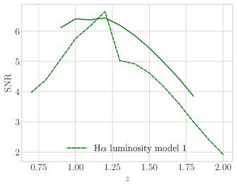
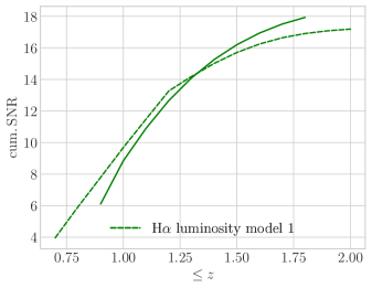
Figure 1: The signal-to-noise ratio (left: per redshift bin, right: cumulative) of the general relativistic bispectrum for a Euclid-like survey with luminosity Model 1 (red) and Model 3 (black) i.e GR contributions with no local primordial non-Gaussianity ($f_{\mathrm{NL}}=0).$

The results are displayed in Fig. 1, which interestingly show that even with a smaller redshift range, Model 3 achieves a slightly better SNR than Model 1. The full information matrix forecast results for both models applied to Roman and Euclid-like, the two surveys targeting H$\alpha$ emitters, are given in Section 4.

Survey	Redshift range	Sky area [$\mathrm{deg}^{2}$]
Roman-like	Model 1 & 3: $0.5\leq z\leq 2$	$2000$
DESI BGS	$0\leq z\leq 0.7$	$14\,000$
Euclid-like	Model 1: $0.7\leq z\leq 2$ Model 3: $0.9\leq z\leq 1.8$	$15\,000$
MegaMapper LBG	$2\leq z\leq 5$	$20\,000$

Table 1: Scope of chosen mock surveys

For our analysis we use cosmological parameters from Planck 2018 data [79]: $h=0.6766$, $\varOmega_{\rm m0}=0.3111$, $\varOmega_{\rm b0}\,h^{2}=0.02242$, $\varOmega_{\rm c0}\,h^{2}=0.11933$, $n_{\rm s}=0.9665$, $\sigma_{8}=0.8102$, $\gamma=0.545$, $\varOmega_{K0}=0=\varOmega_{\nu 0}$. The comoving survey volume is given by

$$V=\frac{4}{3}\,\pi\,f_{\rm sky}\,\left[r(z+\varDelta z/2)^{3}-r(z-\varDelta z/2)^{3}\right]\;,$$ (3.16)

with $f_{\rm sky}$ the fraction of surveyed sky, $r(z)$ the radial comoving distance to redshift $z$ and $\varDelta z$ the width of the redshift bin. The galaxy number density $n_{\rm g}$, magnification bias $\mathcal{Q}$ and evolution bias $\mathcal{E}$ however are dependent on the luminosity function specific to the survey. The explicit implementations for deriving these values for our H$\alpha$ surveys (Euclid/Roman-like) and K-corrected survey (DESI BGS) are outlined in [78]. We obtained the MegaMapper LBG values by taking the Schechter function form for the UV luminosity function and best-fit parameters from table 3 of [80]. The survey-specific input parameters are given in this paper in Appendix C.

4 Results

Following Section 3 and its subsequent subsections on the methodology, we compare the results of the Fisher matrix analysis outlined in Section 3.2 applied to the 6 survey specifications outlined in Section 3.5. That is, Roman-like Model 1, Roman-like Model 3, DESI BGS, Euclid-like Model 1, Euclid-like Model 3 and MegaMapper LBG. The analysis is done for $f_{\mathrm{NL}}=0$, firstly comparing the surveys’ SNR using the formalism set out in Section 3.1 for the total general relativistic contribution (Fig. 2) and the second order general relativistic contribution (Fig. 3).

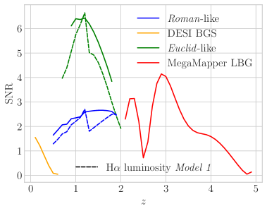
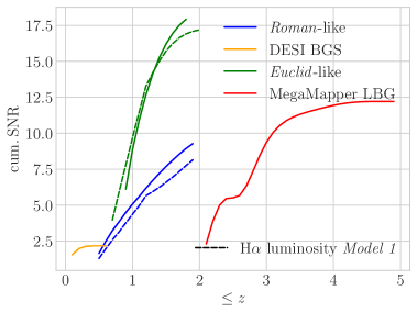
Figure 2: Signal-to-noise ratio for the general relativistic contributions to the galaxy bispectrum for each survey. The dashed blue and green dashed line represent the Model 1 parameters for the $\mathrm{H}\alpha$ surveys, Roman and Euclid-like respectively.

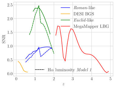
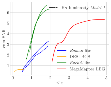
Figure 3: Same as Fig. 2 but for only the second order GR corrections.

From these plots we can clearly see the promise of a detectable GR signal with current surveys, with the expception of DESI BGS and with particularly high expectations from a Euclid-like survey. Naively, we would expect a larger signal from MegaMapper LBG considering it’s larger redshift range and therefore ability to probe small $k$’s well beyond the equality scale, however our analysis shows that the GR signal is significantly suppressed by the evolution bias, $\mathcal{E}$. We find for the second order GR bispectrum we can expect a total SNR of $\sim 6$ with a Euclid-like survey as seen in Fig. 3. It is interesting to note that the SNR for $\mathrm{H}\alpha$ surveys, Euclid and Roman-like, using luminosity Model 3 is larger than for luminosity Model 1 in both examples, even with a smaller redshift range in the case of a Euclid-like survey.

This is largely in agreement with the results of the fisher information matrix analysis on the parameter space $\theta=\{\epsilon_{\rm GR}^{(1)},\epsilon_{\mathrm{GR}}^{(2)},f_{\mathrm{NL}}\}$ as outlined in Section 3.2 and Section 3.3. The marginal errors are given in Fig. 4, showing the comparatively impressive capacity of a Euclid-like survey in accurately detecting the general relativistic signal at both orders achieving a total marginal error $\sigma(\epsilon_{\mathrm{GR}}^{(1)})<0.2$ and $\sigma(\epsilon_{\mathrm{GR}}^{(2)})<0.3$. Our results show that MegaMapper LBG would not improve on the accuracy of the relativistic detection, being comparable with a Roman-like survey even with the vastly larger survey scope, as predicted by the SNR. We note that H$\alpha$ luminosity Model 1 appears to yield a smaller margin of error for $f_{\mathrm{NL}}$, particularly for a Euclid-like survey.

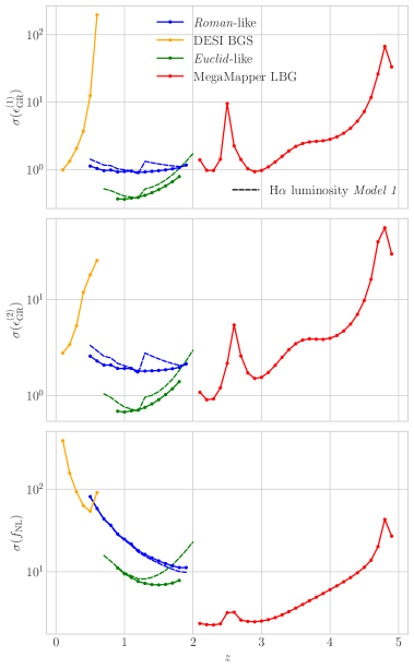
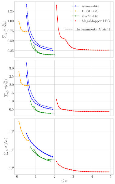
Figure 4: Marginal errors (left: per redshift bin, right: cumulative) on the parameters $\epsilon_{\mathrm{GR}^{(1)}}$, $\epsilon_{\mathrm{GR}^{(2)}}$ and $f_{\mathrm{NL}}$ for $f_{\mathrm{NL}}=0$.

Survey	$\sigma(\epsilon_{\mathrm{GR}}^{(1)})$	$\sigma(\epsilon_{\mathrm{GR}}^{(2)})$	$\sigma(f_{\mathrm{NL}})$
Roman-like Model 1	0.290	0.580	3.994
Roman-like Model 3	0.256	0.502	4.331
DESI BGS	0.723	1.938	33.256
Euclid-like Model 1	0.145	0.233	1.234
Euclid-like Model 3	0.142	0.257	2.446
MegaMapper LBG	0.262	0.364	0.620

Table 2: Marginal errors on each parameter of our chosen parameter space $\theta=\{\epsilon_{\rm GR}^{(1)},\epsilon_{\mathrm{GR}}^{(2)},f_{\mathrm{NL}}\}$ for each survey

However, a significant improvement in accuracy on $f_{\mathrm{NL}}$ can be achieved at the high redshift range reached by MegaMapper LBG, giving a total $\sigma(f_{\mathrm{NL}})<0.7$. The total marginal errors are displayed in Table 2 for $f_{\mathrm{NL}}=0$. The constraints on our parameters can be seen in Fig. 5.

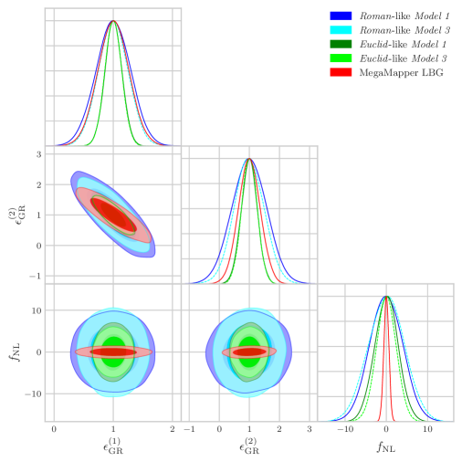
Figure 5: Parameter constraints for each survey (we omit DESI BGS for clarity as the constraints are weak)

Implementing the parameter bias analysis of Section 3.4 for $-5<f_{\mathrm{NL}}<5$ yields Fig. 6. We show the biases for the total information matrix, i.e the sum over all redshift bins. The top plot shows the bias that the assumed value of $f_{\mathrm{NL}}$ compared to the true value $f_{\mathrm{NL}}=0$ has on the measurements of the first order GR amplitude $\epsilon_{\mathrm{GR}}^{(1)}$ in terms of the total marginal error and the middle plot shows the same for the second order GR amplitude $\epsilon_{\mathrm{GR}}^{(2)}$ i.e Section 3.4. The bottom plot shows the bias on $f_{\mathrm{NL}}$ if GR corrections to the bispectrum are ignored i.e Eq. 3.15. We can see that the impact on the measurement of both GR amplitudes $\epsilon_{\rm GR}^{(i)}$, where $i=1,2$, when inaccurate in $f_{\mathrm{NL}}$ is $<0.1\sigma(\epsilon_{\rm GR})^{(i)}$ i.e negligible for all surveys apart from MegaMapper LBG, where the shifts are $<0.6\sigma(\epsilon_{\rm GR}^{(1)})$ and $<1.3\sigma(\epsilon_{\rm GR}^{(2)})$. Since these larger shift values are at the extremities of the analysis, this is not too concerning, as up to $f_{\mathrm{NL}}=\pm 2$ the shifts are $<0.3\sigma(\epsilon_{\rm GR}^{(1)})$ and $<0.5\sigma(\epsilon_{\rm GR}^{(2)})$. Conversely, from the bottom plot, we can see that precise and accurate measurements of $f_{\mathrm{NL}}$ rely on our inclusion of GR corrections in our analysis with surveys probing the larger scales at higher redshift, causing up to $2\sigma(f_{\mathrm{NL}})$ discrepancy in measurement from our most promising survey results, when not included.

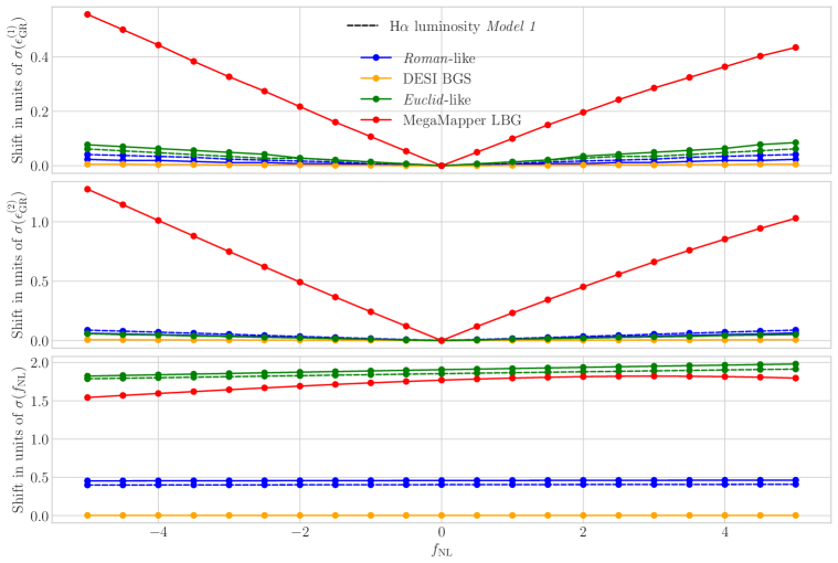
Figure 6: Total parameter bias of each survey in units of marginal errors for $\epsilon_{\mathrm{GR}}^{(1)}$ (top), $\epsilon_{\mathrm{GR}}^{(2)}$ (centre) and $f_{\mathrm{NL}}$ (bottom) for $-5\leq f_{\mathrm{NL}}\leq 5$

This bias for each survey can be seen in Fig. 7. Here we take the true value of $f_{\mathrm{NL}}=-0.9\pm 5.1$ as measured by Planck 2018 [15], shown by the grey vertical line and shaded region representing the error. The shifted (or biased) values of $f_{\mathrm{NL}}$ for each survey are plotted along with the error bars given by the Fisher matrix of the form Eq. 3.10 in the Newtonian regime, i.e inserting Eq. 2.4 for $B_{\rm gN}$ into Eq. 3.9, neglecting all GR and local PNG corrections. This plot demonstrates the importance of including GR corrections in constraining local PNG. The value of $f_{\mathrm{NL}}$ for a Euclid-like survey is shifted to the edge of the margin of error given by Planck 2018, with errors bars extending beyond it. From a quick glance we can see that the surveys with larger error bars have less $f_{\mathrm{NL}}$ bias induced in the Newtonian regime. However, the error bars are significantly larger, and extend outside the margin of error for Planck 2018. Once again, we can see how MegaMapper LBG does not follow this reasoning, due to it’s lower signal detection of GR contributions and higher accuracy on $f_{\mathrm{NL}}$.

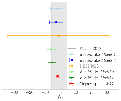
Figure 7: We show the shift on the value of $f_{\mathrm{NL}}$ induced by neglecting GR corrections with error bars in the Newtonian regime. Here we have taken the true value of $f_{\mathrm{NL}}$ as that measured by Planck 2018 [15], $f_{\mathrm{NL}}=-0.9\pm 5.1$, indicated by the grey vertical line and shaded area.

5 Conclusion

The main conclusion that can be drawn from our analysis is that the higher the detection of the GR signal, the more important it is to account for GR corrections when constraining $f_{\rm NL}$. This is shown most convincingly through Fig. 7. The least promising survey from our analysis, with the lowest accuracy for all three parameters, is the DESI BGS, which appears to be inept at detecting any GR corrections to the galaxy bispectrum within a reasonable margin of error and while this means little bias on $f_{\rm NL}$, it also means a huge uncertainty in the measurement of $f_{\rm NL}$ compared to samples at greater depth, see Fig. 5. Comparing the results for the Roman and Euclid-like samples demonstrate that survey depth is more significant than sky coverage in analysis of the interplay between relativistic effects and PNG, however sky coverage does increase the signal of GR contributions and accuracy of the detection of all parameters. These two surveys are the fairest comparison of this since they target the same sample type and thus use the same luminosity functions, therefore the only difference between their analysis is the survey volume, or specifically survey sky area since they probe similar redshift ranges. From Figs. 6 and 7, we see the bias on $f_{\rm NL}$ induced by the Newtonian regime is far more significant then for the lower detection of DESI BGS, while the error bars are much smaller. The smaller scope of a Roman-like survey provides a lower SNR for the GR corrections which in turn gives a lower accuracy in the detection of their amplitudes (see Fig. 4). The MegaMapper LBG sample is not well suited to analyse relativistic contributions to the galaxy bispectrum, as we can see from the disappointingly small SNR in Figs. 2 and 3. We believe the suppression of this signal is caused by the fluctuation of the evolution bias $\mathcal{E}$ from positive to negative values (see Appendices C and 8(d)) as derived from the luminosity model Appendix B. The imprint of the evolution bias is evident for all the surveys, the H$\alpha$ Model 1 discontinuity appears clearly in both Roman and Euclid-like Model 1 SNR analyses. Similarly for MegaMapper LBG, the sharp decrease in the SNR at $z\sim 2.65$ is where $\mathcal{E}$ goes from positive to negative, whereas the redshift bins in which $\mathcal{E}$ is negative $2.7<z<4.5$, produces the highest signal. MegaMapper LBG survey is however well suited to measure fnl to high accuracy as can be seen by the bottom two plots of Fig. 4. We have double checked this by computing the SNR for PNG corrections to the bispectrum i.e $B_{\rm NG}=B_{\rm g}-(B_{\rm gN}+B_{\rm gGR})$ for $f_{\mathrm{NL}}=-0.9$ as in Panck 2018, and found that the SNR for the PNG corrections to the MegaMapper LBG sample is about 4 times higher than that of Euclid-like Model 3. This dynamic is further shown in computing the bias on $f_{\mathrm{NL}}$, as shown in Fig. 6. Both Euclid-like and MegaMapper LBG induce an almost $2\sigma$ shift on $f_{\rm NL}$. The implications of this are only really seen in Fig. 7, where the shift on Euclid-like measurements of $f_{\rm NL}$ is the large whereas MegaMapper LBG shows a very small shift on $f_{\rm NL}$ with margins of error well within that of Planck. This implies that, as the modelling currently stands, constraining $f_{\mathrm{NL}}$ with a relativistic analysis of MegaMapper LBG would not be improvement on the Newtonian analysis, whereas GR corrections are a significant inclusion when studying local PNG through the Euclid-like galaxy bispectrum. We still have hope for MegaMapper LBG’s ability to detect relativistic effects since it will explore the high redshift regime and therefore the ultra large scales beyond the equality scale at which relativistic effects are most dominant and primordial non-Gaussianity can be probed most accuarately. Our study shows that this may be achieved through further developments of the luminosity function, drawing from Halo Occupation Distibutions (HODs) from simulations. This in turn may reduce the suppression of the evolution bias and allow for higher SNR of the GR corrections to the galaxy bispectrum.

Appendix A Fourier kernels and biases

A.1 Fourier kernels

$$F_{2}\left(a,\bm{k}_{1},\bm{k}_{2}\right) =1+\frac{F(a)}{D(a)^{2}}+\left(\frac{k_{1}}{k_{2}}+\frac{k_{2}}{k_{1}}\right)\hat{\bm{k}}_{1}\cdot\hat{\bm{k}}_{2}+\left[1-\frac{F(a)}{D(a)^{2}}\right]\left(\hat{\bm{k}}_{1}\cdot\hat{\bm{k}}_{2}\right)^{2},$$ (A.1)

$$G_{2}\left(\bm{k}_{1},\bm{k}_{2}\right) =\frac{F^{\prime}}{DD^{\prime}}+\left(\frac{k_{1}}{k_{2}}+\frac{k_{2}}{k_{1}}\right)\hat{\bm{k}}_{1}\cdot\hat{\bm{k}}_{2}+\left(2-\frac{F^{\prime}}{DD^{\prime}}\right)\left(\hat{\bm{k}}_{1}\cdot\hat{\bm{k}}_{2}\right)^{2}$$ (A.2)

$$S_{2}\left(\bm{k}_{1},\bm{k}_{2}\right) =\left(\hat{\bm{k}}_{1}\cdot\hat{\bm{k}}_{2}\right)^{2}-\frac{1}{3}$$ (A.3)

$$N_{2}\left(\bm{k}_{1},\bm{k}_{2}\right) =\frac{1}{2}\left(\frac{k_{1}}{k_{2}\mathcal{M}_{1}}+\frac{k_{2}}{k_{1}\mathcal{M}_{2}}\right)\hat{\bm{k}}_{1}\cdot\hat{\bm{k}}_{2}\,,$$ (A.4)

where we use the Einstein-de Sitter relations $F/D^{2}=3/7$ and $F^{\prime}/DD^{\prime}=6/7$ as a reasonable approximation for $\varLambda\mathrm{CDM}$.

A.2 Gaussian clustering biases

$$\rm{\textbf{{Euclid/Roman:}}}\;b_{10} =0.9+0.4z$$ (A.5)

$$b_{20} =-0.741-0.125z+0.123z^{2}+0.00637z^{3}$$ (A.6)

$$\mathbf{DESI\;BGS:}\;b_{10} =1.34/D(z)$$ (A.7)

$$b_{20} =0.30-0.79\,b_{10}+0.20\,b_{10}^{2}+(0.12/b_{10})$$ (A.8)

$$\mathbf{MegaMapper\;LBG:}\;b_{10} =-1.37(1+z)+0.11(1+z)^{2}$$ (A.9)

$$b_{20} =0.30-0.79\,b_{10}+0.20\,b_{10}^{2}+(0.12/b_{10})$$ (A.10)

A.3 non-Gaussian biases

$$b_{01} =2f_{\mathrm{NL}}\delta_{\text{crit }}\left(b_{10}-1\right)$$ (A.11)

$$b_{11} =4f_{\mathrm{NL}}\left[\delta_{\text{crit }}b_{20}+\left(\frac{13}{21}\delta_{\text{crit }}-1\right)\left(b_{10}-1\right)+1\right],$$ (A.12)

$$b_{n} =4f_{\mathrm{NL}}\left[\delta_{\text{crit }}\left(1-b_{10}\right)+1\right],$$ (A.13)

$$b_{02} =4f_{\mathrm{NL}}^{2}\delta_{\text{crit }}\left[\delta_{\text{crit }}b_{20}-2\left(\frac{4}{21}\delta_{\text{crit }}+1\right)\left(b_{10}-1\right)\right].$$ (A.14)

Appendix B MegaMapper LBG biases

To derive the comoving galaxy number density $n_{\mathrm{g}}$, magnification bias $\mathcal{Q}$ and evolution bias $\mathcal{E}$ for the MegaMapper LBG sample we must first start with the luminosity function. We use the Schechter type UV luminosity function with absolute magnitude [80],

$$\varPhi\left(M_{\mathrm{UV}}\right)dM_{\mathrm{UV}}=\left(\frac{\ln 10}{2.5}\right)\phi^{\star}10^{-0.4(1+\alpha)\left(M_{\mathrm{UV}}-M_{\mathrm{UV}}^{\star}\right)}\exp\left(-10^{-0.4\left(M_{\mathrm{UV}}-M_{\mathrm{UV}}^{*}\right)}\right)dM_{\mathrm{UV}},$$ (B.1)

where

$$M_{UV}=m-5\log_{10}\left(\frac{D_{L}(z)}{10\mathrm{pc}}\right)+2.5\log_{10}(1+z)+\underbrace{m_{UV}-m}_{\approx 0}.$$ (B.2)

The last two terms $m_{UV}-m$ is the K-correction and is negligible for the MegaMapper LBG sample so we choose to ignore it. $D_{L}(z)$ is the comoving luminosity distance the best-fit parameters for equation Eq. B.1 are given by table 3 of [80] and printed here in Table 3. We refer you to this paper for a full description of the properties of LBG’s and the selection process.

$z_{\text{eff }}$	$M_{\mathrm{UV}}^{*}$	$\phi^{*}/\left(10h^{-1}\mathrm{Mpc}\right)^{-3}$	$\alpha$	$m_{UV}^{\star}$
2.0	-20.60	9.70	-1.60	24.2
3.0	-20.86	5.04	-1.78	24.7
3.8	-20.63	9.25	-1.57	25.4
4.9	-20.96	3.22	-1.60	25.5
5.9	-20.91	1.64	-1.87	25.8

Table 3: Luminsity function best-fit parameters as given by [80] where you can find references for deriving the best-fit values at each redshift.

As the table values are sparse across the redshift range, we use a cubic spline function to smooth them. This gives us the luminosity function as can be seen in Fig. 8(a). In order to derive the comoving number density, evolution bias and magnification bias, we follow [78], specifically the section on surveys with K-corrections applied to a DESI like survey. The comoving number density is given by (see Fig. 8(b)),

$$n_{\mathrm{g}}\left(z,M_{\mathrm{c}}\right)=\int_{-\infty}^{M_{\mathrm{c}}(z)}\mathrm{d}M\varPhi(z,M),$$ (B.3)

where $M_{\mathrm{c}}$ is given by Eq. B.2 for $m=m_{\mathrm{c}}=24.5$. The magnification bias is given by the relation (see Fig. 8(c)),

$$\mathcal{Q}\left(z,M_{\mathrm{c}}\right)=\frac{5}{2}\frac{\partial\log_{10}n_{\mathrm{g}}\left(z,M_{\mathrm{c}}\right)}{\partial M_{\mathrm{c}}}=\frac{5}{2\ln 10}\frac{\varPhi\left(z,M_{\mathrm{c}}\right)}{n_{\mathrm{g}}\left(z,M_{\mathrm{c}}\right)},$$ (B.4)

and the evolution bias is calculated by (see Fig. 8(d))

$$\mathcal{E}=-\frac{\mathrm{d}\ln n_{\mathrm{g}}}{\mathrm{d}\ln(1+z)}-2\left[1+\frac{1+z}{rH}+\frac{2\ln 10}{5}\frac{\mathrm{d}K}{\mathrm{~{}d}\ln(1+z)}\right]\mathcal{Q}.$$ (B.5)

Since $\mathrm{d}K\approx 0$, the last term in the expression can be ignored.

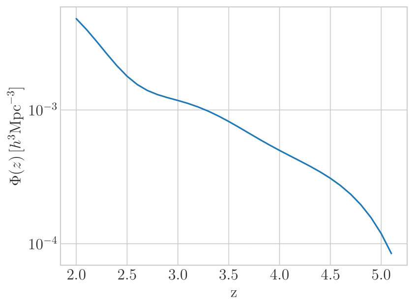
(a) Luminosity function

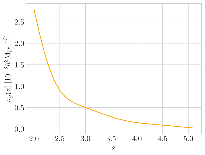
(b) Comoving number density

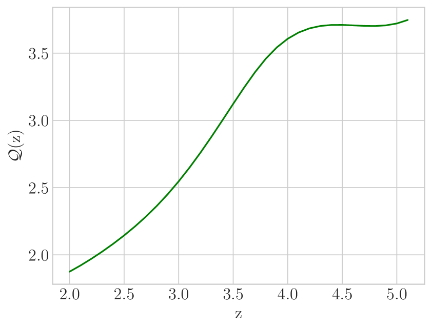
(c) Magnification bias

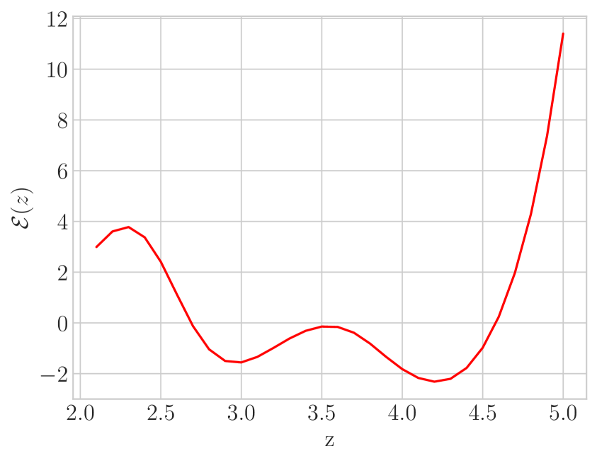
(d) Evolution bias

Figure 8: MegaMapper LBG survey specifications derived from [80, 78].

Appendix C Survey Parameters

$z$	$V(\mathrm{h}^{-3}\,\mathrm{Gpc}^{3})$	$n_{g}(10^{-3}\,\mathrm{h}^{3}\,\mathrm{Mpc}^{-3})$	$\mathcal{E}$	$Q$
0.5	0.24	16.15	$-2.64$	0.81
0.6	0.31	13.21	$-2.82$	0.90
0.7	0.37	11.05	$-2.99$	0.99
0.8	0.43	9.40	$-3.17$	1.08
0.9	0.49	8.09	$-3.35$	1.17
1.0	0.54	7.04	$-3.52$	1.25
1.1	0.58	6.19	$-3.69$	1.34
1.2	0.62	5.48	$-3.86$	1.42
1.3	0.65	4.89	$-2.03$	1.50
1.4	0.68	4.03	$-2.19$	1.58
1.5	0.71	3.35	$-2.35$	1.66
1.6	0.73	2.81	$-2.50$	1.74
1.7	0.74	2.28	$-2.65$	1.81
1.8	0.76	2.02	$-2.80$	1.89
1.9	0.77	1.74	$-2.93$	1.96

Table 4: Survey parameters for Roman-like luminosity Model 1 ($F_{c}=1\times 10^{-16}\mathrm{erg}\,\mathrm{cm}^{-2}\,\mathrm{s}^{-1}$).

$z$	$V(\mathrm{h}^{-3}\,\mathrm{Gpc}^{3})$	$n_{g}(10^{-3}\,\mathrm{h}^{3}\,\mathrm{Mpc}^{-3})$	$\mathcal{E}$	$Q$
0.5	0.24	9.33	$-4.91$	1.07
0.6	0.31	7.82	$-4.71$	1.14
0.7	0.37	6.65	$-4.53$	1.21
0.8	0.43	5.70	$-4.34$	1.29
0.9	0.49	4.90	$-4.24$	1.36
1.0	0.54	4.22	$-4.12$	1.44
1.1	0.58	3.64	$-4.02$	1.52
1.2	0.62	3.13	$-3.92$	1.60
1.3	0.65	2.69	$-3.84$	1.69
1.4	0.68	2.31	$-3.76$	1.77
1.5	0.71	1.97	$-3.68$	1.85
1.6	0.73	1.69	$-3.60$	1.93
1.7	0.74	1.44	$-3.53$	2.01
1.8	0.76	1.23	$-3.45$	2.09
1.9	0.77	1.05	$-3.37$	2.16

Table 5: Survey parameters for Roman-like luminosity Model 3 ($F_{c}=1\times 10^{-16}\mathrm{erg}\,\mathrm{cm}^{-2}\,\mathrm{s}^{-1}$).

$z$	$V(\mathrm{h}^{-3}\,\mathrm{Gpc}^{3})$	$n_{g}(10^{-3}\,\mathrm{h}^{3}\,\mathrm{Mpc}^{-3})$	$\mathcal{E}$	$Q$
0.1	0.05	38.38	$-2.66$	0.55
0.2	0.19	15.88	$-2.90$	0.94
0.3	0.38	6.42	$-3.46$	1.50
0.4	0.60	2.17	$-4.74$	2.31
0.5	0.84	0.56	$-6.01$	3.44
0.6	1.08	0.10	$-7.70$	4.94

Table 6: DESI BGS survey parameters.

$z$	$V(\mathrm{h}^{-3}\,\mathrm{Gpc}^{3})$	$n_{g}(10^{-3}\,\mathrm{h}^{3}\,\mathrm{Mpc}^{-3})$	$\mathcal{E}$	$Q$
0.7	2.78	2.72	$-4.33$	1.66
0.8	3.23	1.98	$-4.76$	1.87
0.9	3.65	1.46	$-5.19$	2.09
1.0	4.03	1.09	$-5.62$	2.30
1.1	4.36	0.82	$-6.05$	2.52
1.2	4.65	0.62	$-6.48$	2.73
1.3	4.90	0.48	$-4.91$	2.94
1.4	5.12	0.34	$-5.33$	3.15
1.5	5.30	0.25	$-5.74$	3.35
1.6	5.45	0.18	$-6.15$	3.56
1.7	5.58	0.13	$-6.55$	3.76
1.8	5.68	0.10	$-6.94$	3.95
1.9	5.76	0.07	$-7.32$	4.14
2.0	5.83	0.06	$-7.69$	4.33

Table 7: Survey parameters for Euclid-like luminosity Model 1 benchmark flux cut ($F_{c}=3\times 10^{-16}\mathrm{erg}\,\mathrm{cm}^{-2}\,\mathrm{s}^{-1}$).

$z$	$V(\mathrm{h}^{-3}\,\mathrm{Gpc}^{3})$	$n_{g}(10^{-3}\,\mathrm{h}^{3}\,\mathrm{Mpc}^{-3})$	$\mathcal{E}$	$Q$
0.9	3.65	1.56	$-6.13$	1.97
1.0	4.03	1.26	$-5.93$	2.07
1.1	4.36	1.02	$-5.73$	2.17
1.2	4.65	0.82	$-5.53$	2.26
1.3	4.90	0.67	$-5.32$	2.34
1.4	5.12	0.54	$-5.11$	2.41
1.5	5.30	0.44	$-4.91$	2.47
1.6	5.45	0.36	$-4.71$	2.52
1.7	5.58	0.29	$-4.51$	2.57
1.8	5.68	0.24	$-4.32$	2.61

Table 8: Survey parameters for Euclid-like luminosity Model 3 benchmark flux cut ($F_{c}=2\times 10^{-16}\mathrm{erg}\,\mathrm{cm}^{-2}\,\mathrm{s}^{-1}$).

$z$	$V(\mathrm{h}^{-3}\,\mathrm{Gpc}^{3})$	$n_{g}(10^{-6}\,\mathrm{h}^{3}\,\mathrm{Mpc}^{-3})$	$\mathcal{E}$	$Q$
2.1	7.88	2.26	2.99	1.92
2.2	7.92	1.79	3.61	1.97
2.3	7.94	1.41	3.78	2.02
2.4	7.95	1.12	3.37	2.08
2.5	7.95	0.91	2.41	2.14
2.6	7.94	0.76	1.12	2.21
2.7	7.91	0.66	-0.13	2.28
2.8	7.88	0.60	-1.04	2.36
2.9	7.84	0.55	-1.50	2.45
3.0	7.80	0.50	-1.56	2.55
3.1	7.74	0.46	-1.34	2.65
3.2	7.69	0.41	-0.99	2.76
3.3	7.63	0.37	-0.61	2.88
3.4	7.57	0.33	-0.31	3.00
3.5	7.50	0.29	-0.14	3.12
3.6	7.43	0.25	-0.16	3.24
3.7	7.36	0.22	-0.39	3.36
3.8	7.29	0.19	-0.81	3.46
3.9	7.22	0.17	-1.34	3.54
4.0	7.15	0.15	-1.82	3.61
4.1	7.07	0.14	-2.17	3.65
4.2	7.00	0.12	-2.32	3.68
4.3	6.93	0.11	-2.20	3.70
4.4	6.85	0.10	-1.78	3.71
4.5	6.78	0.09	-0.98	3.71
4.6	6.70	0.08	-0.24	3.71
4.7	6.63	0.07	1.97	3.70
4.8	6.56	0.06	4.29	3.70
4.9	6.48	0.05	7.37	3.71
5.0	6.41	0.03	11.40	3.72

Table 9: MegaMapper LBG survey parameters.

Appendix D $\beta$ functions

$$\frac{\beta_{1}}{\mathcal{H}^{4}} =\frac{9}{4}\varOmega_{m}^{2}\left[6-2f\left(2\mathcal{E}-4\mathcal{Q}-\frac{4(1-\mathcal{Q})}{\chi\mathcal{H}}-\frac{2\mathcal{H}^{\prime}}{\mathcal{H}^{2}}\right)-\frac{2f^{\prime}}{\mathcal{H}}+\mathcal{E}^{2}+5\mathcal{E}-8\mathcal{E}\mathcal{Q}+4\mathcal{Q}+16\mathcal{Q}^{2}\right.$$

$$\quad-16\frac{\partial\mathcal{Q}}{\partial\ln L}-8\frac{\mathcal{Q}^{\prime}}{\mathcal{H}}+\frac{\mathcal{E}^{\prime}}{\mathcal{H}}+\frac{2}{\chi^{2}\mathcal{H}^{2}}\left(1-\mathcal{Q}+2\mathcal{Q}^{2}-2\frac{\partial\mathcal{Q}}{\partial\ln L}\right)$$

$$\quad-\frac{2}{\chi\mathcal{H}}\left(3+2\mathcal{E}-2\mathcal{E}\mathcal{Q}-3\mathcal{Q}+8\mathcal{Q}^{2}-\frac{3\mathcal{H}^{\prime}}{\mathcal{H}^{2}}(1-\mathcal{Q})-8\frac{\partial\mathcal{Q}}{\partial\ln L}-2\frac{\mathcal{Q}^{\prime}}{\mathcal{H}}\right)$$

$$\quad\left.+\frac{\mathcal{H}^{\prime}}{\mathcal{H}^{2}}\left(-7-2\mathcal{E}+8\mathcal{Q}+\frac{3\mathcal{H}^{\prime}}{\mathcal{H}^{2}}\right)-\frac{\mathcal{H}^{\prime\prime}}{\mathcal{H}^{3}}\right]$$

$$\quad+\frac{3}{2}\varOmega_{m}f\left[5-2f\left(4-\mathcal{E}\right)+\frac{2f^{\prime}}{\mathcal{H}}+2\mathcal{E}\left(5+\frac{2(1-\mathcal{Q})}{\chi_{\mathcal{H}}}\right)-\frac{2\mathcal{E}^{\prime}}{\mathcal{H}}-2\mathcal{E}^{2}+8\mathcal{E}\mathcal{Q}-28\mathcal{Q}\right.$$

$$\quad\left.-\frac{14(1-\mathcal{Q})}{\chi\mathcal{H}}-\frac{3\mathcal{H}^{\prime}}{\mathcal{H}^{2}}+4\left(2-\frac{1}{\chi\mathcal{H}}\right)\frac{\mathcal{Q}^{\prime}}{\mathcal{H}}\right]$$

$$\quad+\frac{3}{2}\varOmega_{m}f^{2}\left[-2+2f-\mathcal{E}+4\mathcal{Q}+\frac{2(1-\mathcal{Q})}{\chi\mathcal{H}}+\frac{3\mathcal{H}^{\prime}}{\mathcal{H}^{2}}\right]$$

$$\quad+f^{2}\left[12-7\mathcal{E}+\mathcal{E}^{2}+\frac{\mathcal{E}^{\prime}}{\mathcal{H}}+\left(\mathcal{E}-3\right)\frac{\mathcal{H}^{\prime}}{\mathcal{H}^{2}}\right]-\frac{3}{2}\varOmega_{m}\frac{f^{\prime}}{\mathcal{H}}$$ (D.1)

$$\frac{\beta_{2}}{\mathcal{H}^{4}} =\frac{9}{2}\varOmega_{m}^{2}\left[-1+\mathcal{E}-2\mathcal{Q}-\frac{2(1-\mathcal{Q})}{\chi\mathcal{H}}-\frac{\mathcal{H}^{\prime}}{\mathcal{H}^{2}}\right]+3\varOmega_{m}f\left[-1+2f-\mathcal{E}+4\mathcal{Q}+\frac{2(1-\mathcal{Q})}{\chi\mathcal{H}}+\frac{3\mathcal{H}^{\prime}}{\mathcal{H}^{2}}\right]$$

$$\quad+3\varOmega_{m}f^{2}\left[-1+\mathcal{E}-2\mathcal{Q}-\frac{2(1-\mathcal{Q})}{\chi\mathcal{H}}-\frac{\mathcal{H}^{\prime}}{\mathcal{H}^{2}}\right]+3\varOmega_{m}\frac{f^{\prime}}{\mathcal{H}}$$ (D.2)

$$\frac{\beta_{3}}{\mathcal{H}^{3}} =\frac{9}{4}\varOmega_{m}^{2}(f-2+2\mathcal{Q})+\frac{3}{2}\varOmega_{m}f\left[-2-f\left(-3+f+2\mathcal{E}-3\mathcal{Q}-\frac{4(1-\mathcal{Q})}{\chi\mathcal{H}}-\frac{2\mathcal{H}^{\prime}}{\mathcal{H}^{2}}\right)-\frac{f^{\prime}}{\mathcal{H}}\right.$$

$$\quad+3\mathcal{E}+\mathcal{E}^{2}-6\mathcal{E}\mathcal{Q}+4\mathcal{Q}+8\mathcal{Q}^{2}-8\frac{\partial\mathcal{Q}}{\partial\ln L}-6\frac{\mathcal{Q}^{\prime}}{\mathcal{H}}+\frac{\mathcal{E}^{\prime}}{\mathcal{H}}$$

$$\quad+\frac{2}{\chi^{2}\mathcal{H}^{2}}\left(1-\mathcal{Q}+2\mathcal{Q}^{2}-2\frac{\partial\mathcal{Q}}{\partial\ln L}\right)+\frac{2}{\chi\mathcal{H}}\left(-1-2\mathcal{E}+2\mathcal{E}\mathcal{Q}+\mathcal{Q}-6\mathcal{Q}^{2}\right.$$

$$\quad\left.\left.+\frac{3\mathcal{H}^{\prime}}{\mathcal{H}^{2}}(1-\mathcal{Q})+6\frac{\partial\mathcal{Q}}{\partial\ln L}+2\frac{\mathcal{Q}^{\prime}}{\mathcal{H}}\right)-\frac{\mathcal{H}^{\prime}}{\mathcal{H}^{2}}\left(3+2\mathcal{E}-6\mathcal{Q}-\frac{3\mathcal{H}^{\prime}}{\mathcal{H}^{2}}\right)-\frac{\mathcal{H}^{\prime\prime}}{\mathcal{H}^{3}}\right]$$

$$\quad+f^{2}\left[-3+2\mathcal{E}\left(2+\frac{(1-\mathcal{Q})}{\chi\mathcal{H}}\right)-\mathcal{E}^{2}+2\mathcal{E}\mathcal{Q}-6\mathcal{Q}-\frac{\mathcal{E}^{\prime}}{\mathcal{H}}-\frac{6(1-\mathcal{Q})}{\chi\mathcal{H}}+2\left(1-\frac{1}{\chi\mathcal{H}}\right)\frac{\mathcal{Q}^{\prime}}{\mathcal{H}}\right]$$ (D.3)

$$\frac{\beta_{4}}{\mathcal{H}^{3}} =\frac{9}{2}\varOmega_{m}f\left[-\mathcal{E}+2\mathcal{Q}+\frac{2(1-\mathcal{Q})}{\chi\mathcal{H}}+\frac{\mathcal{H}^{\prime}}{\mathcal{H}^{2}}\right]$$ (D.4)

$$\frac{\beta_{5}}{\mathcal{H}^{3}} =3\varOmega_{m}f\left[\mathcal{E}-2\mathcal{Q}-\frac{2(1-\mathcal{Q})}{\chi\mathcal{H}}-\frac{\mathcal{H}^{\prime}}{\mathcal{H}^{2}}\right]$$ (D.5)

$$\frac{\beta_{6}}{\mathcal{H}^{2}} =\frac{3}{2}\varOmega_{m}\left[2-2f+\mathcal{E}-4\mathcal{Q}-\frac{2(1-\mathcal{Q})}{\chi\mathcal{H}}-\frac{\mathcal{H}^{\prime}}{\mathcal{H}^{2}}\right]$$ (D.6)

$$\frac{\beta_{7}}{\mathcal{H}^{2}} =f\left(3-\mathcal{E}\right)$$ (D.7)

$$\frac{\beta_{8}}{\mathcal{H}^{2}} =3\varOmega_{m}f(2-f-2\mathcal{Q})+f^{2}\left[4+\mathcal{E}-\mathcal{E}^{2}+4\mathcal{E}\mathcal{Q}-6\mathcal{Q}-4\mathcal{Q}^{2}+4\frac{\partial\mathcal{Q}}{\partial\ln L}+4\frac{\mathcal{Q}^{\prime}}{\mathcal{H}}-\frac{\mathcal{E}^{\prime}}{\mathcal{H}}\right.$$

$$\quad-\frac{2}{\chi^{2}\mathcal{H}^{2}}\left(1-\mathcal{Q}+2\mathcal{Q}^{2}-2\frac{\partial\mathcal{Q}}{\partial\ln L}\right)-\frac{2}{\chi\mathcal{H}}\left(3-2\mathcal{E}+2\mathcal{E}\mathcal{Q}-\mathcal{Q}-4\mathcal{Q}^{2}+\frac{3\mathcal{H}^{\prime}}{\mathcal{H}^{2}}(1-\mathcal{Q})\right.$$

$$\quad\left.\left.+4\frac{\partial\mathcal{Q}}{\partial\ln L}+2\frac{\mathcal{Q}^{\prime}}{\mathcal{H}}\right)-\frac{\mathcal{H}^{\prime}}{\mathcal{H}^{2}}\left(3-2\mathcal{E}+4\mathcal{Q}+\frac{3\mathcal{H}^{\prime}}{\mathcal{H}^{2}}\right)+\frac{\mathcal{H}^{\prime\prime}}{\mathcal{H}^{3}}\right]$$ (D.8)

$$\frac{\beta_{9}}{\mathcal{H}^{2}} =-\frac{9}{2}\varOmega_{m}f$$ (D.9)

$$\frac{\beta_{10}}{\mathcal{H}^{2}} =3\varOmega_{m}f$$ (D.10)

$$\frac{\beta_{11}}{\mathcal{H}^{2}} =\frac{3}{2}\varOmega_{m}\left(1+\frac{2f}{3\varOmega_{m}}\right)+3\varOmega_{m}f-f^{2}\left[-1+\mathcal{E}-2\mathcal{Q}-\frac{2(1-\mathcal{Q})}{\chi\mathcal{H}}-\frac{\mathcal{H}^{\prime}}{\mathcal{H}^{2}}\right]$$ (D.11)

$$\frac{\beta_{12}}{\mathcal{H}^{2}} =-3\varOmega_{m}\left(1+\frac{2f}{3\varOmega_{m}}\right)-f\left[b_{10}\left(f-3+\mathcal{E}\right)+\frac{b_{10}^{\prime}}{\mathcal{H}}\right]$$

$$\quad+\frac{3}{2}\varOmega_{m}\left[b_{10}\left(2+\mathcal{E}-4\mathcal{Q}-\frac{2(1-\mathcal{Q})}{\chi\mathcal{H}}-\frac{\mathcal{H}^{\prime}}{\mathcal{H}^{2}}\right)+\frac{b_{10}^{\prime}}{\mathcal{H}}+2\left(2-\frac{1}{\chi\mathcal{H}}\right)\frac{\partial b_{10}}{\partial\ln L}\right]$$ (D.12)

$$\frac{\beta_{13}}{\mathcal{H}^{2}} =\frac{9}{4}\varOmega_{m}^{2}+\frac{3}{2}\varOmega_{m}f\left[1-2f+2\mathcal{E}-6\mathcal{Q}-\frac{4(1-\mathcal{Q})}{\chi\mathcal{H}}-\frac{3\mathcal{H}^{\prime}}{\mathcal{H}^{2}}\right]+f^{2}\left(3-\mathcal{E}\right)$$ (D.13)

$$\frac{\beta_{14}}{\mathcal{H}} =-\frac{3}{2}\varOmega_{m}b_{10}$$ (D.14)

$$\frac{\beta_{15}}{\mathcal{H}} =2f^{2}$$ (D.15)

$$\frac{\beta_{16}}{\mathcal{H}} =f\left[b_{10}\left(f+\mathcal{E}-2\mathcal{Q}-\frac{2(1-\mathcal{Q})}{\chi\mathcal{H}}-\frac{\mathcal{H}^{\prime}}{\mathcal{H}^{2}}\right)+\frac{b_{10}^{\prime}}{\mathcal{H}}+2\left(1-\frac{1}{\chi\mathcal{H}}\right)\frac{\partial b_{10}}{\partial\ln L}\right]$$ (D.16)

$$\frac{\beta_{17}}{\mathcal{H}} =-\frac{3}{2}\varOmega_{m}f$$ (D.17)

$$\frac{\beta_{18}}{\mathcal{H}} =\frac{3}{2}\varOmega_{m}f-f^{2}\left[3-2\mathcal{E}+4\mathcal{Q}+\frac{4(1-\mathcal{Q})}{\chi\mathcal{H}}+\frac{3\mathcal{H}^{\prime}}{\mathcal{H}^{2}}\right]$$ (D.18)

$$\frac{\beta_{19}}{\mathcal{H}} =f\left[\mathcal{E}-2Q-\frac{2(1-\mathcal{Q})}{\chi\mathcal{H}}-\frac{\mathcal{H}^{\prime}}{\mathcal{H}^{2}}\right]$$ (D.19)

Appendix E $\varUpsilon$ functions

$$\frac{1}{f_{\mathrm{NL}}}\frac{\varUpsilon_{1}}{\mathcal{H}^{2}} =2\left(3-\mathcal{E}\right)f+3\varOmega_{m}\left[1+\mathcal{E}-4\mathcal{Q}-\frac{2(1-\mathcal{Q})}{\chi\mathcal{H}}-\frac{\mathcal{H}^{\prime}}{\mathcal{H}^{2}}\right]$$

$$\quad+\frac{6\varOmega_{m}}{\left(3\varOmega_{m}+2f\right)}\left[\frac{f^{\prime}}{\mathcal{H}}+\left(1+2\frac{\mathcal{H}^{\prime}}{\mathcal{H}^{2}}\right)f\right]$$ (E.1)

$$\frac{1}{f_{\mathrm{NL}}}\frac{\varUpsilon_{2}}{\mathcal{H}} =2f\left[\mathcal{E}-2\mathcal{Q}-\frac{2(1-\mathcal{Q})}{\chi\mathcal{H}}-\frac{\mathcal{H}^{\prime}}{\mathcal{H}^{2}}\right]$$ (E.2)

$$\frac{1}{b_{01}}\frac{\varUpsilon_{3}}{\mathcal{H}^{2}} =\frac{3}{2}\varOmega_{m}\left[2+\mathcal{E}-4\mathcal{Q}+\frac{2(1-\mathcal{Q})}{\chi\mathcal{H}}+\frac{\mathcal{H}^{\prime}}{\mathcal{H}^{2}}+2\left(2-\frac{1}{\chi\mathcal{H}}\right)\frac{\partial\ln b_{01}}{\partial\ln L}\right]$$

$$\quad+f\left[3-f-\mathcal{E}+\frac{1}{2}\frac{\partial\ln b_{01}}{\partial\ln a}\right]$$ (E.3)

$$\frac{1}{b_{01}}\frac{\varUpsilon_{4}}{\mathcal{H}} =-\frac{3}{2}\varOmega_{m}$$ (E.4)

$$\frac{1}{b_{01}}\frac{\varUpsilon_{5}}{\mathcal{H}} =f\left[f+\mathcal{E}-2\mathcal{Q}-\frac{2(1-\mathcal{Q})}{\chi\mathcal{H}}-\frac{\mathcal{H}^{\prime}}{\mathcal{H}^{2}}+2\left(2-\frac{1}{\chi\mathcal{H}}\right)\frac{\partial\ln b_{01}}{\partial\ln L}\right]$$ (E.5)

References

- [1] DESI collaboration, The DESI Experiment Part I: Science,Targeting, and Survey Design, 1611.00036.
- [2] C. Hahn, M.J. Wilson, O. Ruiz-Macias, S. Cole, D.H. Weinberg, J. Moustakas et al., The DESI Bright Galaxy Survey: Final Target Selection, Design, and Validation, AJ 165 (2023) 253 [2208.08512].
- [3] L. Amendola et al., Cosmology and fundamental physics with the Euclid satellite, Living Rev. Rel. 21 (2018) 2 [1606.00180].
- [4] Euclid Collaboration, Y. Mellier, Abdurro’uf, J.A. Acevedo Barroso, A. Achúcarro, J. Adamek et al., Euclid. I. Overview of the Euclid mission, arXiv e-prints (2024) arXiv:2405.13491 [2405.13491].
- [5] D. Spergel, N. Gehrels, C. Baltay, D. Bennett, J. Breckinridge, M. Donahue et al., Wide-Field InfrarRed Survey Telescope-Astrophysics Focused Telescope Assets WFIRST-AFTA 2015 Report, arXiv e-prints (2015) arXiv:1503.03757 [1503.03757].
- [6] T. Eifler, H. Miyatake, E. Krause, C. Heinrich, V. Miranda, C. Hirata et al., Cosmology with the Roman Space Telescope - multiprobe strategies, MNRAS 507 (2021) 1746 [2004.05271].
- [7] D.J. Schlegel et al., The MegaMapper: A Stage-5 Spectroscopic Instrument Concept for the Study of Inflation and Dark Energy, 2209.04322.
- [8] S. Camera, R. Maartens and M.G. Santos, Einstein’s legacy in galaxy surveys., MNRAS 451 (2015) L80 [1412.4781].
- [9] O. Umeh, S. Jolicoeur, R. Maartens and C. Clarkson, A general relativistic signature in the galaxy bispectrum: the local effects of observing on the lightcone, JCAP 2017 (2017) 034 [1610.03351].
- [10] D. Jeong, F. Schmidt and C.M. Hirata, Large-scale clustering of galaxies in general relativity, PRD 85 (2012) 023504 [1107.5427].
- [11] M. Bruni, R. Crittenden, K. Koyama, R. Maartens, C. Pitrou and D. Wands, Disentangling non-Gaussianity, bias and GR effects in the galaxy distribution, Phys. Rev. D 85 (2012) 041301 [1106.3999].
- [12] A. Kehagias, A. Moradinezhad Dizgah, J. Noreña, H. Perrier and A. Riotto, A Consistency Relation for the Observed Galaxy Bispectrum and the Local non-Gaussianity from Relativistic Corrections, JCAP 08 (2015) 018 [1503.04467].
- [13] S. Jolicoeur, O. Umeh, R. Maartens and C. Clarkson, Imprints of local lightcone \projection effects on the galaxy bispectrum. Part II, JCAP 2017 (2017) 040 [1703.09630].
- [14] K. Koyama, O. Umeh, R. Maartens and D. Bertacca, The observed galaxy bispectrum from single-field inflation in the squeezed limit, JCAP 07 (2018) 050 [1805.09189].
- [15] Planck Collaboration, Y. Akrami, F. Arroja, M. Ashdown, J. Aumont, C. Baccigalupi et al., Planck 2018 results. IX. Constraints on primordial non-Gaussianity, A&A 641 (2020) A9 [1905.05697].
- [16] N. Kaiser, Clustering in real space and in redshift space, MNRAS 227 (1987) 1.
- [17] C. Bonvin, Isolating relativistic effects in large-scale structure, Class. Quant. Grav. 31 (2014) 234002 [1409.2224].
- [18] C. Bonvin and R. Durrer, What galaxy surveys really measure, PRD 84 (2011) 063505 [1105.5280].
- [19] A. Challinor and A. Lewis, Linear power spectrum of observed source number counts, PRD 84 (2011) 043516 [1105.5292].
- [20] J. Yoo, A.L. Fitzpatrick and M. Zaldarriaga, New perspective on galaxy clustering as a cosmological probe: General relativistic effects, PRD 80 (2009) 083514 [0907.0707].
- [21] J. Fonseca, S. Camera, M. Santos and R. Maartens, Hunting down horizon-scale effects with multi-wavelength surveys, Astrophys. J. Lett. 812 (2015) L22 [1507.04605].
- [22] D. Alonso, P. Bull, P.G. Ferreira, R. Maartens and M. Santos, Ultra large-scale cosmology in next-generation experiments with single tracers, Astrophys. J. 814 (2015) 145 [1505.07596].
- [23] L. Lopez-Honorez, O. Mena and S. Rigolin, Biases on cosmological parameters by general relativity effects, PRD 85 (2012) 023511 [1109.5117].
- [24] J. Yoo, N. Hamaus, U. Seljak and M. Zaldarriaga, Going beyond the Kaiser redshift-space distortion formula: a full general relativistic account of the effects and their detectability in galaxy clustering, arXiv e-prints (2012) arXiv:1206.5809 [1206.5809].
- [25] A. Raccanelli, D. Bertacca, O. Doré and R. Maartens, Large-scale 3D galaxy correlation function and non-Gaussianity, JCAP 08 (2014) 022 [1306.6646].
- [26] S. Camera, M.G. Santos and R. Maartens, Probing primordial non-Gaussianity with SKA galaxy redshift surveys: a fully relativistic analysis, Mon. Not. Roy. Astron. Soc. 448 (2015) 1035 [1409.8286].
- [27] A. Raccanelli, F. Montanari, D. Bertacca, O. Doré and R. Durrer, Cosmological Measurements with General Relativistic Galaxy Correlations, JCAP 05 (2016) 009 [1505.06179].
- [28] D. Alonso and P.G. Ferreira, Constraining ultralarge-scale cosmology with multiple tracers in optical and radio surveys, Phys. Rev. D 92 (2015) 063525 [1507.03550].
- [29] J. Fonseca, R. Maartens and M.G. Santos, Probing the primordial Universe with MeerKAT and DES, Mon. Not. Roy. Astron. Soc. 466 (2017) 2780 [1611.01322].
- [30] L.R. Abramo and D. Bertacca, Disentangling the effects of Doppler velocity and primordial non-Gaussianity in galaxy power spectra, Phys. Rev. D 96 (2017) 123535 [1706.01834].
- [31] C.S. Lorenz, D. Alonso and P.G. Ferreira, Impact of relativistic effects on cosmological parameter estimation, Phys. Rev. D 97 (2018) 023537 [1710.02477].
- [32] J. Fonseca, R. Maartens and M.G. Santos, Synergies between intensity maps of hydrogen lines, Mon. Not. Roy. Astron. Soc. 479 (2018) 3490 [1803.07077].
- [33] M. Ballardini, W.L. Matthewson and R. Maartens, Constraining primordial non-Gaussianity using two galaxy surveys and CMB lensing, Mon. Not. Roy. Astron. Soc. 489 (2019) 1950 [1906.04730].
- [34] N. Grimm, F. Scaccabarozzi, J. Yoo, S.G. Biern and J.-O. Gong, Galaxy Power Spectrum in General Relativity, JCAP 11 (2020) 064 [2005.06484].
- [35] J.L. Bernal, N. Bellomo, A. Raccanelli and L. Verde, Beware of commonly used approximations. Part II. Estimating systematic biases in the best-fit parameters, JCAP 10 (2020) 017 [2005.09666].
- [36] M.S. Wang, F. Beutler and D. Bacon, Impact of Relativistic Effects on the Primordial Non-Gaussianity Signature in the Large-Scale Clustering of Quasars, Mon. Not. Roy. Astron. Soc. 499 (2020) 2598 [2007.01802].
- [37] T. Baldauf, U. Seljak and L. Senatore, Primordial non-Gaussianity in the bispectrum of the halo density field, JCAP 2011 (2011) 006 [1011.1513].
- [38] V. Desjacques, D. Jeong and F. Schmidt, Large-Scale Galaxy Bias, Phys. Rept. 733 (2018) 1 [1611.09787].
- [39] M. Tellarini, A.J. Ross, G. Tasinato and D. Wands, Galaxy bispectrum, primordial non-Gaussianity and redshift space distortions, JCAP 06 (2016) 014 [1603.06814].
- [40] L. Verde, L.-M. Wang, A. Heavens and M. Kamionkowski, Large scale structure, the cosmic microwave background, and primordial non-gaussianity, Mon. Not. Roy. Astron. Soc. 313 (2000) L141 [astro-ph/9906301].
- [41] R. Scoccimarro, E. Sefusatti and M. Zaldarriaga, Probing primordial non-Gaussianity with large - scale structure, Phys. Rev. D 69 (2004) 103513 [astro-ph/0312286].
- [42] E. Sefusatti, M. Crocce, S. Pueblas and R. Scoccimarro, Cosmology and the Bispectrum, Phys. Rev. D 74 (2006) 023522 [astro-ph/0604505].
- [43] E. Sefusatti and E. Komatsu, The Bispectrum of Galaxies from High-Redshift Galaxy Surveys: Primordial Non-Gaussianity and Non-Linear Galaxy Bias, Phys. Rev. D 76 (2007) 083004 [0705.0343].
- [44] T. Giannantonio and C. Porciani, Structure formation from non-Gaussian initial conditions: Multivariate biasing, statistics, and comparison with N-body simulations, PRD 81 (2010) 063530 [0911.0017].
- [45] M. Tellarini, A.J. Ross, G. Tasinato and D. Wands, Non-local bias in the halo bispectrum with primordial non-Gaussianity, JCAP 07 (2015) 004 [1504.00324].
- [46] C.A. Watkinson, S. Majumdar, J.R. Pritchard and R. Mondal, A fast estimator for the bispectrum and beyond – a practical method for measuring non-Gaussianity in 21-cm maps, Mon. Not. Roy. Astron. Soc. 472 (2017) 2436 [1705.06284].
- [47] S. Majumdar, J.R. Pritchard, R. Mondal, C.A. Watkinson, S. Bharadwaj and G. Mellema, Quantifying the non-Gaussianity in the EoR 21-cm signal through bispectrum, Mon. Not. Roy. Astron. Soc. 476 (2018) 4007 [1708.08458].
- [48] D. Karagiannis, A. Lazanu, M. Liguori, A. Raccanelli, N. Bartolo and L. Verde, Constraining primordial non-Gaussianity with bispectrum and power spectrum from upcoming optical and radio surveys, Mon. Not. Roy. Astron. Soc. 478 (2018) 1341 [1801.09280].
- [49] V. Yankelevich and C. Porciani, Cosmological information in the redshift-space bispectrum, Mon. Not. Roy. Astron. Soc. 483 (2019) 2078 [1807.07076].
- [50] D. Sarkar, S. Majumdar and S. Bharadwaj, Modelling the post-reionization neutral hydrogen () 21-cm bispectrum, Mon. Not. Roy. Astron. Soc. 490 (2019) 2880 [1907.01819].
- [51] D. Karagiannis, A. Slosar and M. Liguori, Forecasts on Primordial non-Gaussianity from 21 cm Intensity Mapping experiments, JCAP 11 (2020) 052 [1911.03964].
- [52] S. Bharadwaj, A. Mazumdar and D. Sarkar, Quantifying the Redshift Space Distortion of the Bispectrum I: Primordial Non-Gaussianity, Mon. Not. Roy. Astron. Soc. 493 (2020) 594 [2001.10243].
- [53] D. Karagiannis, J. Fonseca, R. Maartens and S. Camera, Probing primordial non-Gaussianity with the power spectrum and bispectrum of future 21 cm intensity maps, Phys. Dark Univ. 32 (2021) 100821 [2010.07034].
- [54] A. Moradinezhad Dizgah, M. Biagetti, E. Sefusatti, V. Desjacques and J. Noreña, Primordial Non-Gaussianity from Biased Tracers: Likelihood Analysis of Real-Space Power Spectrum and Bispectrum, JCAP 05 (2021) 015 [2010.14523].
- [55] K.S. Dawson, D.J. Schlegel, C.P. Ahn, S.F. Anderson, É. Aubourg, S. Bailey et al., The Baryon Oscillation Spectroscopic Survey of SDSS-III, AJ 145 (2013) 10 [1208.0022].
- [56] eBOSS collaboration, The SDSS-IV extended Baryon Oscillation Spectroscopic Survey: Overview and Early Data, Astron. J. 151 (2016) 44 [1508.04473].
- [57] R. Laureijs, J. Amiaux, S. Arduini, J.L. Auguères, J. Brinchmann, R. Cole et al., Euclid Definition Study Report, arXiv e-prints (2011) arXiv:1110.3193 [1110.3193].
- [58] DESI collaboration, The DESI Experiment, a whitepaper for Snowmass 2013, 1308.0847.
- [59] J.L. Fuentes, J.C. Hidalgo and K.A. Malik, Galaxy number counts at second order: an independent approach, Class. Quant. Grav. 38 (2021) 065014 [1908.08400].
- [60] J. Yoo and M. Zaldarriaga, Beyond the Linear-Order Relativistic Effect in Galaxy Clustering: Second-Order Gauge-Invariant Formalism, Phys. Rev. D 90 (2014) 023513 [1406.4140].
- [61] E. Di Dio, R. Durrer, G. Marozzi and F. Montanari, Galaxy number counts to second order and their bispectrum, JCAP 12 (2014) 017 [1407.0376].
- [62] D. Bertacca, R. Maartens and C. Clarkson, Observed galaxy number counts on the lightcone up to second order: II. Derivation, JCAP 11 (2014) 013 [1406.0319].
- [63] D. Bertacca, Observed galaxy number counts on the light cone up to second order: III. Magnification bias, Class. Quant. Grav. 32 (2015) 195011 [1409.2024].
- [64] O. Umeh, K. Koyama, R. Maartens, F. Schmidt and C. Clarkson, General relativistic effects in the galaxy bias at second order, JCAP 05 (2019) 020 [1901.07460].
- [65] O. Umeh and K. Koyama, The galaxy bias at second order in general relativity with Non-Gaussian initial conditions, JCAP 12 (2019) 048 [1907.08094].
- [66] N. Dalal, O. Dore, D. Huterer and A. Shirokov, The imprints of primordial non-gaussianities on large-scale structure: scale dependent bias and abundance of virialized objects, Phys. Rev. D 77 (2008) 123514 [0710.4560].
- [67] S. Matarrese and L. Verde, The effect of primordial non-Gaussianity on halo bias, Astrophys. J. Lett. 677 (2008) L77 [0801.4826].
- [68] R. Maartens, S. Jolicoeur, O. Umeh, E.M. De Weerd, C. Clarkson and S. Camera, Detecting the relativistic galaxy bispectrum, JCAP 03 (2020) 065 [1911.02398].
- [69] E.M. de Weerd, C. Clarkson, S. Jolicoeur, R. Maartens and O. Umeh, Multipoles of the relativistic galaxy bispectrum, JCAP 05 (2020) 018 [1912.11016].
- [70] C. Clarkson, E.M. de Weerd, S. Jolicoeur, R. Maartens and O. Umeh, The dipole of the galaxy bispectrum, Mon. Not. Roy. Astron. Soc. 486 (2019) L101 [1812.09512].
- [71] S. Jolicoeur, R. Maartens, E.M. De Weerd, O. Umeh, C. Clarkson and S. Camera, Detecting the relativistic bispectrum in 21cm intensity maps, JCAP 06 (2021) 039 [2009.06197].
- [72] S. Jolicoeur, O. Umeh, R. Maartens and C. Clarkson, Imprints of local lightcone projection effects on the galaxy bispectrum. Part III. Relativistic corrections from nonlinear dynamical evolution on large-scales, JCAP 03 (2018) 036 [1711.01812].
- [73] S. Jolicoeur, A. Allahyari, C. Clarkson, J. Larena, O. Umeh and R. Maartens, Imprints of local lightcone projection effects on the galaxy bispectrum IV: second-order vector and tensor contributions, JCAP 2019 (2019) 004 [1811.05458].
- [74] O. Umeh, K. Koyama and R. Crittenden, Testing the equivalence principle on cosmological scales using the odd multipoles of galaxy cross-power spectrum and bispectrum, JCAP 08 (2021) 049 [2011.05876].
- [75] R. Maartens, S. Jolicoeur, O. Umeh, E.M. De Weerd and C. Clarkson, Local primordial non-Gaussianity in the relativistic galaxy bispectrum, JCAP 04 (2021) 013 [2011.13660].
- [76] A.F. Heavens, T.D. Kitching and L. Verde, On model selection forecasting, dark energy and modified gravity, MNRAS 380 (2007) 1029 [astro-ph/0703191].
- [77] L. Pozzetti, C.M. Hirata, J.E. Geach, A. Cimatti, C. Baugh, O. Cucciati et al., Modelling the number density of H emitters for future spectroscopic near-IR space missions, Astron. Astrophys. 590 (2016) A3 [1603.01453].
- [78] R. Maartens, J. Fonseca, S. Camera, S. Jolicoeur, J.-A. Viljoen and C. Clarkson, Magnification and evolution biases in large-scale structure surveys, JCAP 12 (2021) 009 [2107.13401].
- [79] Planck collaboration, Planck 2018 results. VI. Cosmological parameters, Astron. Astrophys. 641 (2020) A6 [1807.06209].
- [80] M.J. Wilson and M. White, Cosmology with dropout selection: straw-man surveys \& CMB lensing, JCAP 10 (2019) 015 [1904.13378].