Probing populations of dark stellar remnants in the globular clusters 47 Tuc and Terzan 5 using pulsar timing

Abstract

We present a new method to combine multimass equilibrium dynamical models and pulsar timing data to constrain the mass distribution and remnant populations of Milky Way globular clusters (GCs). We first apply this method to 47 Tuc, a cluster for which there exists an abundance of stellar kinematic data and which is also host to a large population of millisecond pulsars. We demonstrate that the pulsar timing data allow us to place strong constraints on the overall mass distribution and remnant populations even without fitting on stellar kinematics. Our models favor a small population of stellar-mass BHs in this cluster (with a total mass of $412\begin{subarray}{c}+77\\ -146\end{subarray}\ \mathrm{M}_{\odot}$), arguing against the need for a large ($>2000\ \mathrm{M}_{\odot}$) central intermediate-mass black hole. We then apply the method to Terzan 5, a heavily obscured bulge cluster which hosts the largest population of millisecond pulsars of any Milky Way GC and for which the collection of conventional stellar kinematic data is very limited. We improve existing constraints on the mass distribution and structural parameters of this cluster and place stringent constraints on its black hole content, finding an upper limit on the mass in BHs of $\sim 4500\ \mathrm{M}_{\odot}$. This method allows us to probe the central dynamics of GCs even in the absence of stellar kinematic data and can be easily applied to other GCs with pulsar timing data, for which datasets will continue to grow with the next generation of radio telescopes.

1 Introduction

Pulsars have a long history of being used to investigate the mass distribution of globular clusters (GCs). Early work from Phinney (1992, 1993) examined the effect of a pulsar’s surroundings on its measured spin ($\dot{P}$) and orbital period derivatives ($\dot{P}_{\rm b}$; for pulsars in binary systems), including quantifying the effects of the cluster potential, Galactic potential, proper motion and intrinsic effects like magnetic breaking. Recently, several works have presented detailed analyses of pulsar data for probing the gravitational potential of GCs (see e.g., Prager et al. 2017 for Terzan 5 (catalog ), Freire et al. 2017 and Abbate et al. 2018, 2019b for 47 Tuc (catalog ), Gieles et al. 2018 for NGC 6624, and Abbate et al. 2019a for M62).

Pulsars indeed present a unique opportunity to probe the central dynamics of these systems, especially when crowding and extinction make it challenging to obtain detailed stellar kinematic data in their central regions. Because of their extremely stable periods (spin and orbital), measured changes in the periods of pulsars beyond their (unknown) intrinsic spin down due to magnetic breaking can be almost entirely attributed to external factors. By performing timing measurements over long time scales and precisely measuring the changes in their periods, we can learn about the host potential of the pulsars. In particular, the observed period derivatives due to the changing ‘Doppler shift’ from the line-of-sight gravitational acceleration felt by pulsars in GCs allow us to constrain the gravitational potential and mass distribution of GCs hosting pulsars.

Most of the studies mentioned above used single-mass dynamical models, without a mass spectrum. Therefore, they cannot capture the effect of mass segregation, which is affected by the presence/absence of central black holes (e.g. Merritt et al., 2004; MacKey et al., 2008; Gill et al., 2008; Peuten et al., 2016, 2017; Weatherford et al., 2018). These studies also usually focus on fitting models to the pulsar data, ignoring the velocity dispersion profiles, surface density profiles and stellar mass functions which are typically used to constrain mass models of GCs. As an example, Freire et al. (2017) presented a single-mass King model of 47 Tuc which was compared to the pulsar acceleration data as well as the measured “jerk" (the time derivative of the acceleration) of the pulsars. Their model does not contain an intermediate-mass black hole (IMBH) but is still able to account for all of the pulsars’ period derivatives as well as the inferred jerks for all the pulsars within the cluster core.

In this work, we present new self-consistent multimass models of 47 Tuc and Terzan 5 that are fitted both to traditional observables (velocity dispersion profiles, number density profile, local stellar mass function observations) and to the variety of pulsar timing data available for these clusters. The direct inclusion of the pulsar data in the likelihood function allows us to revisit and address the previous claim from Kızıltan et al. (2017a) that the pulsar accelerations favor a large central mass in 47 Tuc in the form of an IMBH. We use updated stellar mass function data where available, and adopt the latest constraints on the distance to our clusters from Gaia (Baumgardt & Vasiliev, 2021) as a prior on the distance parameter in our models. To properly model the effect and constrain the size of a possible population of stellar-mass BHs, our multimass models use stellar evolution recipes based on recent prescriptions for the masses and natal kicks of BHs, and can therefore include realistic BH populations. While our models do not explicitly allow for an IMBH, given that the effects of a central IMBH and a large population of centrally concentrated stellar-mass BHs are expected to be similar beyond the sphere of influence of the IMBH, especially when the mass fraction of the cluster in BHs is small (e.g. Aros & Vesperini, 2023), a best-fitting model without a large population of BHs would provide evidence that an IMBH is not required to explain the dynamics of the cluster.

Since we are interested in accurately modeling the present-day mass distribution within these clusters, equilibrium distribution function-based models are a good choice. Compared to the more computationally expensive evolutionary models like Monte-Carlo or $N$-body models (which are limited to relatively small grids), our multimass models offer much-increased flexibility to vary the cluster’s structural properties, stellar mass function, and population of dark remnants (including BHs) at a small fraction of the computational cost.

Both 47 Tuc and Terzan 5 are host to large populations of pulsars. 47 Tuc is a well-studied cluster with a great deal of stellar kinematic data, making it an ideal candidate to test our method. Terzan 5 is a heavily obscured bulge cluster which is host to the largest population of millisecond pulsars of any Milky Way GC and which is located in the bulge, making the collection of conventional stellar kinematic data extremely challenging. The combination of the large pulsar population and the lack of traditional stellar kinematic data means that our method is particularly well-suited to studying the central dynamics of this cluster. This large population of pulsars may be partially explained by the cluster’s collision rate, which is the highest of any Milky Way GC (e.g. Lanzoni et al., 2010). The central dynamics of this cluster are therefore of great interest.

The remainder of this paper is structured as follows. In Section 2 we describe the data to which we fit our models. Section 3 describes the models, fitting procedure and individual likelihoods. In Section 4 we present our fits and discuss our results. In Section 5 we discuss the implications of our results and compare them to other studies. We finally summarize our findings in Section 6.

2 Data

For this study, we use the same data that was used by Dickson et al. (2023, 2024), with the addition of the pulsar data described below and some additional datasets for Terzan 5. We summarize the data below.

2.1 Kinematics and density profiles

2.1.1 Proper motion dispersion profiles

We use both Hubble Space Telescope (HST) proper motion data and Gaia DR3 proper motions to constrain the kinematics of the clusters. For 47 Tuc, there are proper motion measurements from HST that cover the inner regions of the cluster. These data were presented in Libralato et al. (2022) and are split into radial and tangential dispersion profiles, allowing some leverage on the velocity anisotropy of the cluster.

For both clusters, we also use Gaia DR3 proper motion dispersion profiles which are based on the membership catalogs presented in Vasiliev & Baumgardt (2021). These profiles are split into radial and tangential components for 47 Tuc where there is an abundance of high-probability members (the radial and tangential profiles were derived in Dickson et al. 2023), but left as total proper motion ($\mu_{\rm tot}^{2}=\mu_{\alpha^{*}}^{2}+\mu_{\delta}^{2}$) for Terzan 5 where isolating high-probability members is more difficult due to bulge contamination.

2.1.2 Line-of-sight velocity dispersion profiles

We use the line-of-sight velocity dispersion profiles from Baumgardt & Hilker (2018) to further constrain the kinematics of the clusters. These dispersion profiles are based on archival spectra obtained at the European Southern Observatory’s (ESO) Very Large Telescope (VLT) and the Keck observatory, supplemented with published radial velocity data from the literature from Baumgardt (2017).

For 47 Tuc, we additionally use the line-of-sight dispersion profile presented by Kamann et al. (2018), who used the MUSE spectrograph (Bacon et al., 2010) to collect data for 22 GCs.

As these radial velocity samples are dominated by bright stars, we assume that these velocity dispersion profiles trace the kinematics of upper main-sequence and evolved stars (which we assume trace the kinematics of giants) in our models.

2.1.3 Number density profiles

We use the number density profiles from De Boer et al. (2019) and Lanzoni et al. (2010) to constrain the size and structural parameters of the clusters. The De Boer et al. (2019) profile is made up of a combination of the number density profile of cluster members based on Gaia DR2 data in the outer regions and a surface brightness profile from Trager et al. (1995) in the central regions, which is matched to the Gaia number density profile in the region where the two profiles overlap.

Terzan 5 is not included in the compilation of De Boer et al. (2019) due its position in the bulge, where crowding and extinction are significant issues. Because of these challenges, we use the number density profile from Lanzoni et al. (2010) which is based on a combination of data from the HST, the Multi-conjugate Adaptive optics Demonstrator (MAD) on VLT and the Two Micron All Sky Survey (2MASS) which combine to cover the entire radial extent of the cluster.

The Gaia data only includes bright stars ($m>0.6\ \mathrm{M}_{\odot}$) and the HST and ground-based data are likewise dominated by bright stars, so we assume that these number density profiles trace the distribution of upper main-sequence and evolved stars in our models.

Note that there are two density profiles we could have chosen from for Terzan 5: the surface brightness profile of Trager et al. (1995) or the number density profile of Lanzoni et al. (2010). In their region of overlap, these profiles do not match very well with each other, even when scaled vertically. The Lanzoni et al. (2010) profile decreases faster in the outer regions compared to the Trager et al. (1995) profile. We opted to use the Lanzoni et al. (2010) profile because it is based on HST data and modern ground-based data which should help to more reliably subtract bulge contamination, and also because it has well-defined uncertainties. We also found that tests with the surface brightness profile of Trager et al. (1995) resulted in best-fitting models where the surface brightness profile and the other datasets and profiles could not be simultaneously reproduced as well as when using the Lanzoni et al. (2010) number density profile.

2.2 Stellar mass functions

As a constraint on the global present-day stellar mass function of 47 Tuc, we use the completeness-corrected stellar mass function data that was derived from archival HST photometry by Baumgardt et al. (2023). These are based on various archival HST images (20 different pointings for 47 Tuc, proposal IDs shown in Figure 5) from which stellar number counts were derived as a function of magnitude and projected distance from the cluster center and were then converted into stellar mass functions through isochrone fits. For 47 Tuc, there are extensive observations which cover stars within a mass range of $\sim$0.1\text{\,}\mathrm{-}$$0.8\text{\,}\mathrm{M}_{\odot}$$ as well as a radial range of 0-40 arcminutes from the cluster center. The large span of radii and stellar masses allows us to constrain the varying local stellar mass function as a function of distance from the cluster center, and therefore the degree of mass segregation in the cluster.

The stellar mass function for Terzan 5 was derived in the same way as for 47 Tuc, but was not included in the compilation of Baumgardt et al. (2023) due to limitations with the data resulting from the cluster’s position in the bulge. For this cluster, we have a single mass function field, in the infrared (filters F110W and F160W of HST proposal 12933, PI: Ferraro) which covers a region from 0.6-1.6 arcminutes from the cluster center and a mass range of $\sim$0.6\text{\,}\mathrm{-}$$0.9\text{\,}\mathrm{M}_{\odot}$$. While this dataset provides weaker constraints on the model than the mass function data for 47 Tuc, it is still useful for constraining the amount of visible mass in the cluster around its half-mass radius and verifying that the assumed global stellar mass function in our model of Terzan 5 is reasonable.

2.3 Pulsar data

For 47 Tuc, we use timing solutions from Freire et al. (2017), Ridolfi et al. (2016) and Freire & Ridolfi (2018) which include both the spin and orbital periods (the latter when applicable, for pulsars in binaries) and their time derivatives. For Terzan 5, we use the timing solutions presented in Lyne et al. (2000), Ransom et al. (2005), Prager et al. (2017), Cadelano et al. (2018), Andersen & Ransom (2018), Ridolfi et al. (2021) and Padmanabh et al. (2024), again including both the spin and orbital periods and their derivatives, where available.

Pulsars with non-degenerate companions are classified as either ‘black-widow’ or ‘redback’ systems, where black widows have companions with masses less than $\sim 0.08\ \mathrm{M}_{\odot}$ and redbacks have more massive companions. The redbacks are worthy of special attention as they often display changes in their observed spin periods that are likely due to Roche lobe overflow of the companion or interactions between the companion and the pulsar wind (e.g. Thongmeearkom et al., 2024). The observed changes in the periods of these systems could be incorrectly interpreted as effects from the cluster potential, so we follow Prager et al. (2017) and exclude redback systems from our analysis. Among the well-timed pulsars, this means we exclude pulsar W from 47 Tuc and pulsars A, P, ad and ar from Terzan 5. The pulsar data is summarized in Tables 5 and 6 in the Appendix.

Finally, we make use of the Australia Telescope National Facility’s pulsar database presented by Manchester et al. (2005) in order to build a representative population of Galactic MSPs which we use to estimate the probability distribution for the intrinsic spin-down of the pulsars as a function of their spin period (see Section 3.3.1).

3 Methods

3.1 Models

To model the dynamics and mass distribution of 47 Tuc and Terzan 5, we use the gcfit package, recently presented by Dickson et al. (2023, 2024). This package couples a fast mass evolution algorithm with the limepy family of models presented by Gieles & Zocchi (2015). We refer readers to these papers for a detailed description of the models, and provide a brief summary here. The limepy models are a set of distribution function-based equilibrium models that are isothermal for the most bound stars near the cluster center and described by polytropes in the outer regions near the escape energy. The models have been extensively tested against $N$-body models (Zocchi et al., 2016; Peuten et al., 2017) and their multimass version is able to effectively reproduce the effects of mass segregation. Their suitability for mass modeling of GCs has been tested on mock data (Hénault-Brunet et al., 2019), and they have recently been applied to real datasets as well (for example, Gieles et al., 2018; Hénault-Brunet et al., 2020; Dickson et al., 2023, 2024).

The input parameters needed to compute our models include the dimensionless central potential $\phi_{0}$, the truncation parameter $g$, the anisotropy radius $r_{a}$ which determines the degree of radial anisotropy in the models, $\delta$ which sets the mass dependence of the velocity scale and thus governs the degree of mass segregation, and finally the specific mass bins to use as defined by the mean stellar mass ($m_{j}$) and total mass ($M_{j}$) of each bin, which together specify the stellar mass function. In order to scale the model units to physical units, the total mass of the cluster $M$ and a size scale (the half-mass radius of the cluster $r_{\rm h}$) are provided as well. Finally, we provide the distance to the cluster ($D$) which is used in converting between angular and linear quantities.

In order to generate the input mass bins (the $m_{j}$ and $M_{j}$ sets of input values) for the multimass limepy models, the gcfit models use the evolve_mf algorithm, originally presented by Balbinot & Gieles (2018) and updated in Dickson et al. (2023). This algorithm combines precomputed grids of stellar evolution models, isochrones and initial-final mass relations to model the evolution of a given initial mass function (IMF), including the effects of stellar evolution as well as (optionally) mass loss due to escaping stars and dynamical ejections. The algorithm returns a binned mass function at a requested evolutionary time, for specified metallicity, ideal for use as an input in the limepy models.

We parameterize the mass function as a three-segment broken power law with break points at $0.5\ \mathrm{M}_{\odot}$ and $1.0\ \mathrm{M}_{\odot}$. We provide to evolve_mf the IMF slopes ($\alpha_{1}$, $\alpha_{2}$ and $\alpha_{3}$) and break points, the cluster age, metallicity and initial escape velocity. We adopt the same methodology as Dickson et al. (2023) to determine the initial escape velocities of our clusters. Briefly, we run an initial fit with an initial guess of the escape velocity and use the present-day escape velocity of this preliminary fit to set the initial escape velocity of the cluster. We use double the present-day value as our estimate for the initial escape velocity, which accounts for adiabatic expansion of the cluster after mass-loss due to stellar evolution. We note that after the initial fit, changing the initial escape velocity by $20\ \mathrm{km\ s}^{-1}$ in either direction has no discernible effect on the final model. We additionally specify parameters which control the mass loss (if any) due to escaping stars and the specific binning to be used when returning the final discrete mass-function bins. We finally provide the black hole retention fraction ($\mathrm{BH}_{\mathrm{ret}}$) which controls the percentage of the mass in black holes initially created from the initial mass function that is retained to the present day after natal kicks and dynamical ejections (see Dickson et al. 2024 for details). For this study we do not model the mass loss due to escaping stars, so we set this mass loss due to escaping stars to be zero, and we are effectively specifying the present-day mass function for low-mass stars, not their IMF.

3.2 Fitting

The gcfit package provides a uniform interface for fitting the coupled limepy and evolve_mf models to a variety of observables using either a Markov Chain Monte Carlo (MCMC) or nested sampling algorithm. For this work, we use the nested sampling algorithm, which is implemented using the dynesty package (Speagle, 2020; Koposov et al., 2023). For the majority of our parameters we adopt wide, uniform priors, with the exception of the distance where we adopt the measurements of Baumgardt & Vasiliev (2021) as Gaussian priors and the mass function power-law slopes where we adopt the physically motivated priors described in Dickson et al. (2023). We list the priors in Table 1.

Table 1: Model parameters and their priors. Most priors are uniform and are chosen to bound the parameters around a reasonable range of values for both clusters. For the mass function slopes, we add the additional constraint that $\alpha_{2}$ must be steeper than $\alpha_{1}$ and $\alpha_{3}$ steeper than $\alpha_{2}$. For the distance, we use a Gaussian prior with the distance measurement from Baumgardt & Vasiliev (2021) and its uncertainty providing the mean $\mu$ and standard deviation $\sigma$ of the prior. These distances are $D=4.521\pm 0.031$ $\mathrm{k}\mathrm{p}\mathrm{c}$ and $D=6.62\pm 0.15$ $\mathrm{k}\mathrm{p}\mathrm{c}$ for 47 Tuc and Terzan 5 respectively.

Parameter	Prior Form	Value
$\phi_{0}$	Uniform	[0.1, 15]
$M[10^{6}\ \mathrm{M}_{\odot}]$	Uniform	[0.01, 3]
$r_{h}$ [pc]	Uniform	[0.5, 15]
$\log_{10}{\left(r_{a}/{\rm pc}\right)}$	Uniform	[0, 8]
$g$	Uniform	[0, 3.5]
$\delta$	Uniform	[0.3, 0.5]
$s^{2}$	Uniform	[0, 20]
$F$	Uniform	[1, 7.5]
$\alpha_{1}$	Uniform	[-1, 2.35]
$\alpha_{2}$	Uniform	[-1, 2.35] and $\geq\alpha_{1}$
$\alpha_{3}$	Uniform	[1.6, 4] and $\geq\alpha_{2}$
$\mathrm{BH}_{\mathrm{ret}}[\%]$	Uniform	[0, 100]
$D[\mathrm{kpc}]$	Gaussian	BV21

3.3 Likelihoods

The majority of the likelihood functions we use for different datasets are Gaussian likelihoods. Provided below is the log-likelihood for velocity dispersion profile data as an example, but all other likelihoods are of a similar form:

$$\ln\left(\mathcal{L}\right)=-\frac{1}{2}\sum_{i=1}^{N_{\rm p}}\left\{\frac{\left[\sigma_{\mathrm{obs}}(r_{i})-\sigma_{\mathrm{model}}(r_{i})\right]^{2}}{\delta\sigma_{\mathrm{obs}}^{2}(r_{i})}-\ln\left[\delta\sigma_{\mathrm{obs}}^{2}(r_{i})\right]\right\},$$ (1)

where $\mathcal{L}$ is the likelihood, $N_{\rm p}$ is the number of data points, $\sigma_{\mathrm{obs}}$ is the measured velocity dispersion, $\sigma_{\mathrm{model}}$ is the model velocity dispersion at the corresponding radius, $r$ is the projected distance from the cluster center, and $\delta\sigma_{\mathrm{obs}}$ is the uncertainty in the velocity dispersion. The likelihoods for other observables are formulated in the same way, and the specifics are discussed in Dickson et al. (2023) as well as in the gcfit documentation. The total log-likelihood is the sum of all the log-likelihoods for each set of observations.

For the mass function and number density profile likelihoods, we include additional nuisance parameters and scaling terms. For the number density data, we introduce a parameter $s^{2}$ which is added in quadrature to the existing measurement uncertainties. This parameter allows us to add a constant contribution to all values in the dataset, effectively lowering the weight of the data located farthest from the cluster center where the number density is lowest. This allows us to account for limitations in the models such as the effects of potential escapers near the cluster tidal boundary that the limepy models do not account for (see Claydon et al. 2019 for a discussion of potential escapers in equilibrium models).

Finally, for the number density profile data, we make an additional modification to equation  (1) and introduce a scaling factor $K$ which allows us to fit only on the shape of the number density profile instead of the absolute values. $K$ is defined as follows (see section 3.3 of Hénault-Brunet et al. 2020 for a complete explanation) and the model data points ($\Sigma_{\mathrm{model},i}$) are multiplied by this value before they are compared to the data:

$$K=\frac{\sum_{i=1}^{N_{\rm p}}\Sigma(r)_{\mathrm{obs},i}\Sigma(r)_{\mathrm{model},i}/\delta\Sigma(r)_{\mathrm{model},i}^{2}}{\sum_{i=1}^{N_{\rm p}}\left(\Sigma(r)_{\mathrm{model},i}\right)^{2}/\delta\Sigma(r)_{\mathrm{obs},i}^{2}},$$ (2)

where $N_{\rm p}$ is the number of data points, $\Sigma(r)_{\mathrm{obs},i}$ are the number density measurements, $\Sigma(r)_{\mathrm{model},i}$ are the model number densities at the corresponding radii and $\delta\Sigma(r)_{\mathrm{obs},i}$ are the uncertainties on the number density measurements where $r$ is the projected radius of a given measurement of $\Sigma(r)_{\mathrm{obs},i}$.

We discuss the likelihoods for the pulsar timing data and the stellar mass function data separately in the subsections below.

3.3.1 Pulsars

Pulsar period derivatives, as measured by an observer, are made up of several distinct components, with contributions from the cluster’s gravitational potential, the gravitational potential of the Milky Way, the pulsar’s proper motion, intrinsic effects like magnetic breaking, and the changing dispersion measure between the pulsar and the observer. The effects of the cluster’s proper motion and the Galactic potential are fairly well constrained based on the pulsar’s position and motion in the Galaxy but, the effects of processes like magnetic breaking which are intrinsic to the pulsar itself require more careful consideration. The breakdown of the measured period derivative $(\dot{P}/P)_{\rm obs}$ into separate components is:

$$\left(\frac{\dot{P}}{P}\right)_{\rm obs}=\left(\frac{\dot{P}}{P}\right)_{\rm int}+\frac{a_{{\rm cl},z}}{c}+\frac{a_{{\rm G}}}{c}+\frac{a_{\rm S}}{c}+\frac{a_{\mathrm{DM}}}{c},$$ (3)

where $(\dot{P}/P)_{\rm int}$ is any change in period due to the effects intrinsic to the pulsar like magnetic breaking, $c$ is the speed of light, $a_{{\rm cl},z}$ the line-of-sight acceleration of the pulsar due to the cluster’s gravitational potential and is the quantity we are most interested in, $a_{\rm G}$ is the acceleration of the pulsar along the line of sight due to the Galaxy’s gravitational potential, $a_{\rm S}$ is the ‘Shklovskii’ effect (Shklovskii, 1970), an apparent acceleration due to the proper motion of the pulsar and $a_{\mathrm{DM}}$ is the effect of the changing dispersion measure between the pulsar and the observer.

For each of the components in equation (3), we explain below how we calculate either a point estimate or a probability distribution for the quantities of interest, and how we combine these to obtain a probability distribution for the measured period derivative of a pulsar, given a model (i.e. the likelihood).

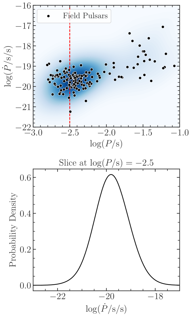
Figure 1: Top: The $P$-$\dot{P}$ plane for the field pulsars with the Gaussian KDE of the $P$-$\dot{P}$ distribution shown in blue. Bottom: an example of a slice from this KDE. The slice is taken at $\log{P}=-2.5$ s and shows the distribution of $\log{\dot{P}}$ values for pulsars with this period.

All pulsars have some intrinsic spin-up or spin-down caused by processes like magnetic breaking or active accretion. We exclude any redback pulsars (pulsars with massive, non-degenerate companions) from this work and therefore assume that none of the pulsars are actively accreting and that any intrinsic effects are purely in the spin-down direction (positive $(\dot{P}/P)_{\rm int}$ term in Equation 3). To estimate the probability distribution for the intrinsic spin-down distribution, we assume that the intrinsic spin-down of cluster pulsars follows the same distribution as the Galactic field pulsars, and that it is dependent only on their period. We use the ATNF pulsar catalog (Manchester et al., 2005) to build a distribution of possible $\dot{P}$ values for a given value of $P$ using the Galactic field pulsars as a reference (for which the period derivative can be directly linked to the intrinsic spin-down after correcting for Galactic and proper motion contributions due to there being no cluster acceleration for these pulsars). We compute a Gaussian kernel density estimator (KDE) in the field $P$-$\dot{P}$ space, which is sliced along each cluster pulsar’s period to extract a distribution of intrinsic values. We show the field pulsars in the $P$-$\dot{P}$ plane, the KDE and an example of a slice from this KDE in Figure 1.

The next two components, $a_{\rm cl}/c$ and $a_{\rm G}/c$, are fundamentally similar in that they are both manifestations of the Doppler effect. In the typical case, we infer a star’s radial velocity by measuring the frequency shift of some known spectral feature, but in the case of pulsars, we instead measure the acceleration of the pulsar along the line of sight by measuring the rate of change of the pulsar’s period.

We will first look at $a_{\rm G}/c$, the effect of the Galaxy’s gravitational potential on the pulsar’s period derivative. The acceleration due to the Galaxy’s potential is a function of the pulsar’s position in the Galaxy and the Galaxy’s mass distribution. We use the Gala package (Price-Whelan, 2017) to calculate the acceleration due to the Galactic potential at each cluster’s position. We adopt the MWPotential2014 potential presented in Bovy (2015) as well as the cluster positions measured by Vasiliev & Baumgardt (2021) who used Gaia EDR3 data to measure the positions (including distances) and kinematics of Milky Way GCs. After projecting this acceleration along the line of sight, the effect on the period derivative is the following:

$$\dot{P}_{\rm G}=\frac{a_{\rm G}P}{c},$$ (4)

where $\dot{P}_{\rm G}$ is the contribution to the period derivative due to the Galactic potential.

The effect of the cluster’s gravitational potential on the pulsar’s period derivative (the $a_{\rm cl}/c$ term in equation 3) is the effect we are most interested in as it helps us to constrain the internal mass distribution of the cluster. For a pulsar with a known 3-D position within the cluster, the period derivative due to the cluster’s gravitational potential ($\dot{P}_{\rm cl}$) will simply be:

$$\dot{P}_{\rm cl}=\frac{a_{{\rm cl},z}P}{c}.$$ (5)

Because the pulsar position along the line of sight is unknown, we need to generate a probability distribution over possible line-of-sight accelerations for a given pulsar at a given projected radius for a given model, based on the enclosed mass over the full range of possible line-of-sight positions. We can then weight this distribution by the probability of a pulsar being at a given position $z$ along the line of sight to generate a probability distribution for $\dot{P}_{\rm cl}$ given a projected radius for a given model.

In order to generate the probability distribution of a pulsar being at a given position along the line of sight we insert a tracer mass bin into the limepy models. This tracer mass bin is a single mass bin with a mean mass of $1.6\ \mathrm{M}_{\odot}$ and a negligible total mass. This allows us to calculate the (line-of-sight) density profile of pulsar-mass objects in our model at a given projected radius. This profile is proportional to the probability that a pulsar has a given line-of-sight acceleration, given the model parameters, which indirectly provides constraints on the position of the pulsar along the line-of-sight. Combining the line-of-sight density profile with the line-of-sight acceleration profile we then obtain a probability distribution over the range of period derivatives for a given projected radius for a given model.

We show the expression from which we can calculate this probability distribution in equation (6):

$$P\left(a_{{\rm cl},z}\mid R_{i}\right)\propto\frac{\mathrm{d}m}{\mathrm{d}a_{{\rm cl},z}}=\frac{\mathrm{d}m}{\mathrm{d}z}\absolutevalue{\frac{\mathrm{d}z}{\mathrm{d}a_{{\rm cl},z}}}=\frac{\rho(z)}{\left|{{\rm d}a_{{\rm cl},z}/{\rm d}z}\right|},$$ (6)

where $P\left(a_{{\rm cl},z}\mid R_{i}\right)$ is the probability of a given line-of-sight acceleration measurement ($a_{{\rm cl},z}$) for a projected radius $R_{i}$, $m$ is mass column density of pulsar-mass objects along the line of sight at projected radius $R_{i}$, $a_{{\rm cl},z}$ is the line-of-sight acceleration for a given line-of-sight position and $\rho(z)$ is the mass density of pulsar-mass objects at a given line-of-sight position. We note that, as stated on the right-hand side of Equation 6, this probability distribution is not normalized. After constructing this distribution, we explicitly normalize it such that it behaves like a probability density function. Each of the quantities on the right-hand side of Equation (6) ($\rho(z)$, ${\rm d}a_{{\rm cl},z}/{\rm d}z$) are calculated for each limepy model. We show the combination of these distributions in Figure 2.

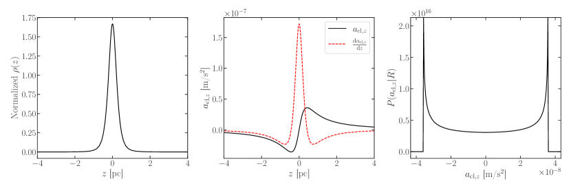
Figure 2: An example of the combination of the line-of-sight density and acceleration profiles leading to the probability distribution of line-of-sight accelerations. Left panel: The normalized line-of-sight density profile for pulsar-mass objects for a model fit to Terzan 5 at the projected radius of pulsar aa. Middle panel: The line-of-sight acceleration profile for the same model and projected radius. The derivative of this profile, used in the calculation of the probability distribution of line-of-sight accelerations is shown with a red, dashed line. Right panel: The probability distribution for the line-of-sight acceleration for the same model, at the same projected radius. This distribution is a result of combining the density profile with the derivative of the acceleration profile.

The Shklovskii effect ($a_{\rm S}/c$) is the effect of the pulsar’s proper motion on its observed period derivative. Any transverse motion of a pulsar acts to increase the distance to the pulsar, regardless of the direction of motion. A constant transverse motion results in a non-linear increase in the distance, manifesting as an apparent line-of-sight acceleration (e.g. Verbiest et al., 2008). This effect is calculated as:

$$\dot{P}_{\rm S}=\frac{a_{\rm S}P}{c}=\frac{\mu^{2}DP}{c},$$ (7)

where $\dot{P}_{\rm S}$ is the rate of change of the period due to the Shklovskii effect and $\mu$ is the proper motion. We use the cluster’s bulk proper motion to calculate this effect and again adopt the measurements of Vasiliev & Baumgardt (2021). Finally, $D$ is the distance to the cluster, one of the parameters which we allow to vary in our fitting. This effect is of order $a_{\rm S}\sim 10^{-11}-10^{-10}\ \mathrm{m\ s^{-2}}$ which is negligible compared the acceleration due to the cluster potential which is of order $10^{-9}-10^{-8}\ \mathrm{m\ s^{-2}}$ (e.g. Figure 2).

The final component, $a_{\rm DM}/c$, is the effect of the changing dispersion measure between a pulsar and the observer. The total amount and distribution of the ionized gas along our line of sight is not necessarily constant over the full time-span over which these observations were performed and small changes in the total dispersion measure between us and the cluster can cause small variations in the observed period derivatives (see, for example, Prager et al. 2017). This effect is stochastic, meaning it is unlikely to bias the timing solution in one direction or the other. Furthermore, the magnitude of this effect is expected to be very small, on the order of $10^{-13}\ \mathrm{m\ s^{-2}}$ (Prager et al., 2017), several orders of magnitude smaller than the typical acceleration from the cluster potential, therefore we do not consider it in our analysis.

One potential contribution to the observed values of $\dot{P}/P$ that we do not model is the acceleration and its higher-order derivatives caused by nearby stars in the dense core of the cluster. For the acceleration of the pulsars in particular, this effect has been shown to be typically $\sim 2$ orders of magnitude smaller than the mean-field acceleration from the cluster potential as a whole (Phinney, 1993; Prager et al., 2017). This effect is however relevant for the higher order derivatives, where nearby stars contribute at a similar level to the bulk cluster potential (Blandford et al., 1987; Gieles et al., 2018). It is for this reason that while higher-order period derivatives are measured for many of the pulsars we use in this work, we chose not to consider these measurements in our determination of the mass distributions of our clusters.

To combine these various effects into a likelihood function for $(\dot{P}/P)_{\rm meas}$ given a model, we start with the distribution of $\dot{P}_{\rm cl}/P$ from the cluster’s gravitational potential and convolve with it the intrinsic distribution of $(\dot{P}/P)_{\rm int}$ values for the period of a given pulsar. We additionally convolve the distribution with a Gaussian distribution, centered at zero with a width equal to the uncertainty of $(\dot{P}/P)_{\rm meas}$ in order to fully incorporate the uncertainty of the period derivative measurement. We then shift this distribution by the point estimates for the contributions of the Galactic potential and the Shklovskii effect. This results in a probability distribution for a measured period derivative which fully incorporates the physical effects within the cluster, which depend on our model parameters as well as the effects of the Galactic gravitational potential and the effects of the pulsars’ proper motions. We use this probability distribution to compute the likelihood of each measured period derivative. We show an example of the combination of these various distributions into the final likelihood in Figure 3.

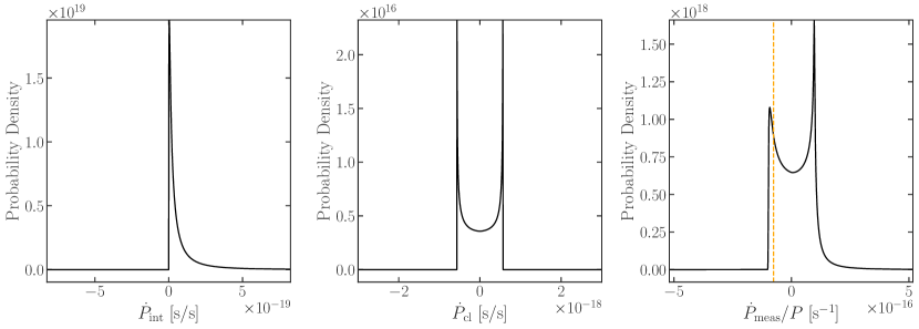
Figure 3: Left panel: The probability distribution of $\dot{P}_{\rm int}$ (intrinsic spin-down) for pulsar aa in Terzan 5. Note that this distribution is of the same form as the one shown in the bottom panel of Figure 1 but here shown on a linear scale. Middle panel: The probability distribution of $\dot{P}_{\rm cl}$ (due to the cluster’s potential at the projected radius of pulsar aa in a model fit to Terzan 5. Right panel: The convolution of the intrinsic and cluster $\dot{P}$ distributions, then convolved with a Gaussian distribution representing the uncertainty on the measured period derivative, transformed to $\dot{P}/P$, with the observed value for pulsar aa shown as a vertical dashed line.

Many pulsars in GCs are in binary systems, and for systems with well-determined timing solutions, the orbital period derivatives of these systems can be measured. The orbital period solutions are useful because the orbital periods of these systems are of the order of days, while the intrinsic orbital decay of these systems acts over millions of years (e.g. Binney & Tremaine, 2008). This means that effects intrinsic to the system are negligible and any measured change in the binary period derivatives can be entirely attributed to the acceleration from the cluster and the well-constrained effects of the Galactic potential and pulsar’s proper motion. Due to the longer timescales and the difficulties associated with determining the orbital periods of these systems (see Ridolfi et al. 2016 for details), the relative uncertainties on the orbital period derivatives are much larger than those of the spin-period derivatives. These larger uncertainties mean that the likelihood functions for the observed orbital period derivatives are wider and provide weaker constraints on the mass distribution of the cluster, but we nonetheless use the orbital period derivatives of these systems (pulsars E, H, I Q, R, S, T, U, X and Y in 47 Tuc and pulsars ao, ap, au, av, aw and ax in Terzan 5) as an additional constraint on the cluster potential, independent of any intrinsic effects on the period derivatives. We construct these likelihood functions in an identical way to the spin period likelihoods but we neglect any effects intrinsic to the binary systems.

One avenue for future improvement of this methodology lies in including the dispersion measures of the pulsars in the analysis. The dispersion measure of a pulsar provides a measure of the amount of ionized gas between the pulsar and an observer, with a higher column density of free electrons producing a larger dispersion measure. Given an estimate of the average dispersion measure between an observer and a cluster and a model for the internal gas distribution within a cluster, the dispersion measures provide an estimate of the line-of-sight position of each pulsar within the cluster.

For 47 Tuc, Abbate et al. (2018) used the pulsars within the cluster to infer the internal gas distribution. These authors found that the pulsar data preferred a uniform gas distribution within the cluster rather than a distribution that follows the stellar density (see also Pancino et al. 2024), finding a gas density $n_{\rm g}$ of $0.23\pm 0.05\ \mathrm{cm^{-3}}$. This measurement, combined with the average cluster dispersion measure $\mathrm{DM_{cl}}$ of $24.38\pm 0.02\ \mathrm{pc\ cm^{-3}}$ allows us to infer the 3-D position of each pulsar within 47 Tuc, independent of our modeling. We describe the necessary modifications to equation 6 in Appendix A.1.

We implemented this alternative formulation and applied it to 47 Tuc to test if the dispersion measures would enable the pulsar timing data to place stronger constraints on the mass distribution within our models. We found that while the dispersion measures did in some cases provide stronger constraints from individual pulsars, the uncertainties on the dispersion-measure-based line-of-sight positions are such that the overall constraints are ultimately very similar to those provided by the density-based calculation described in equation (6). Because the required internal gas models do not yet exist for Terzan 5 and because the dispersion measures provided little to no improvement for 47 Tuc, we opt to simply use the density-based calculation for both clusters for the remainder of this paper.

3.4 Stellar mass functions

The stellar mass function likelihoods are also Gaussian likelihoods, however, care must be taken when extracting model values due to the non-trivial footprint of the observed HST fields from which the mass functions were extracted. To ensure that we are extracting mass functions from the same corresponding regions in the models, we employ a Monte Carlo integration method which allows us to handle the irregular overlapping HST fields. This process is described in detail by Dickson et al. (2023) and is implemented in the gcfit package.

The only uncertainty formally included with the stellar mass function data is the Poisson counting error. We introduce a nuisance parameter $F$ which scales up the uncertainties on the absolute counts by a constant factor, leading to larger relative errors in regions with lower counts. This error encapsulates additional sources of error that may not have been accounted for such as the error associated with the conversion from luminosity to mass with an isochrone and the fact that the mass function is being approximated as a broken power law, a functional form which may not be a perfectly accurate representation of the true mass function of the cluster.

3.5 Stellar populations and mass bins

To generate the input mass bins for the limepy models the evolve_mf algorithm requires as inputs the mass function power-law slopes, as well as the age and metallicity of the stellar population. For 47 Tuc we adopt an age of 11.75 Gyr (VandenBerg et al., 2013) and a metallicity of $[\mathrm{Fe}/\mathrm{H}]=-0.72$ (Harris, 1996, 2010 edition). Depending on the fit, as detailed below, we either allow the mass function power-law slopes to vary or fix the mass function.

Terzan 5 has been found to have at least three distinct stellar populations (Ferraro et al., 2009; Origlia et al., 2013; Ferraro et al., 2016). One of these populations, the most metal-poor population ($[\mathrm{Fe}/\mathrm{H}]=-0.8$), only makes up a small fraction of the cluster and can be neglected in our analysis. The other two population are a young (4.5 Gyr) super-solar ($[\mathrm{Fe}/\mathrm{H}]=0.2$) population, making up about $40\%$ of the cluster (by mass) and an old (12 Gyr) population with $[\mathrm{Fe}/\mathrm{H}]=-0.2$ making up the other $60\%$ of the cluster. With the young population making up a significant fraction of the cluster, we cannot simply assume a single, old stellar population for Terzan 5 as we do for 47 Tuc as we want our remnant populations to be as realistic as possible.

Tests with our stellar evolution algorithm show that this $40/60$ mixture of the young and old stellar populations results in a remnant mass fraction around $35\%$ at the present day, made up of mostly white dwarfs. We can achieve a similar remnant fraction ($\sim 34\%$) with a single metal-poor ($[\mathrm{Fe}/\mathrm{H}]=-0.2$), intermediate-age population of about 8 Gyr. Using this intermediate-age stellar population also makes the main-sequence turnoff mass consistent with the maximum mass of main-sequence stars of $\sim 0.9\ \mathrm{M}_{\odot}$ in our stellar mass function data, avoiding possible issues when comparing the observed mass function and model predictions.

While populations of different metallicities are expected to produce different remnants from similarly massive progenitors, this is a minor effect for our modeling. Our primary goal is to produce a realistic mix of remnants that together make up the correct fraction of the total mass of the cluster, a goal for which an intermediate-age population is a useful simplification.

Finally, the stellar mass function data available for Terzan 5 does not cover a wide enough range of masses or distances from the cluster center to leave the mass function power-law slopes free while fitting as they are derived from a single field and only extend down to $\sim 0.6\ \mathrm{M}_{\odot}$. As such, we chose to fix the mass function slopes for Terzan 5 while still including the mass function data as a constraint on the visible stellar mass in three radial bins between 0.67 and 1.67 arcminutes from the center.

We chose to adopt for the present-day mass function of Terzan 5 the bottom-light IMF of Baumgardt et al. (2023), which was measured from star clusters in the Milky Way and Magellanic Clouds and represents the best estimate for the IMF of massive star clusters. We show in Section 4 that this mass function provides a satisfactory match to the available stellar mass function data. This mass function has slopes of $\alpha_{1}=0.3,\alpha_{2}=1.65,\alpha_{3}=2.3$ and we again place our breakpoints at $0.5$ and $1$ $\mathrm{M}_{\odot}$.

4 Results

To test the performance of our method, we run several fits for each cluster with different subsets of the data introduced in Section 2.

For 47 Tuc, we perform three fits: (1) a fit to all available data for this cluster (47Tuc-AllData), (2) a fit with the pulsar timing data held out (47Tuc-NoPulsars), and (3) a fit to the number density profile, pulsar timing data and a single field of mass function data (47Tuc-NoKin), designed to emulate the data available for Terzan 5.

For Terzan 5 we also run three fits: (1) a fit with all of the available data for this cluster (Ter5-AllData), (2) a fit with the pulsar data held out (Ter5-NoPulsars), and finally (3) a fit on just the number density profile and pulsar data, with the kinematic data and mass function data held out (Ter5-NoKinNoMF), to test the reliability of the limited stellar kinematic data available for Terzan 5.

These fits are summarized in Table 2. We present the median of the posterior probability distribution and $1\sigma$ credibility intervals for the parameters of each of these fits in Table 3.

Table 2: Summary of the different model fits for 47 Tuc and Terzan 5, showing which datasets are included or held out in each case. The columns indicate if the models are fit to the number density profile (NDP), line-of-sight velocity dispersion profile (LOS), proper motion dispersion profile (PM), stellar mass function data (MF) and the pulsar timing data.

Fit	NDP	LOS	PM	MF	Pulsars
47Tuc-AllData	✓	✓	✓	✓	✓
47Tuc-NoPulsars	✓	✓	✓	✓
47Tuc-NoKin	✓			✓(one field)	✓
Ter5-AllData	✓	✓	✓	✓	✓
Ter5-NoPulsars	✓	✓	✓	✓
Ter5-NoKinNoMF	✓				✓

Table 3: Medians and $1\sigma$ uncertainties of each model parameter for each of our fits. Entries without uncertainties indicate parameters that have been held fixed during fitting. We note that as discussed in Dickson et al. (2023), the statistical uncertainties listed here likely underestimate the true uncertainties on each parameter and, in particular, our uncertainties on the cluster mass are likely closer to $10\%$ (Dickson et al., 2024).

Cluster	47Tuc-AllData	47Tuc-NoPulsars	47Tuc-NoKin	Ter5-AllData	Ter5-NoPulsars	Ter5-NoKinNoMF
$\hat{\phi}_{0}$	$6.08\begin{subarray}{c}+0.07\\ -0.08\end{subarray}$	$6.12\begin{subarray}{c}+0.06\\ -0.07\end{subarray}$	$5.99\begin{subarray}{c}+0.14\\ -0.05\end{subarray}$	$5.9\begin{subarray}{c}+0.3\\ -0.3\end{subarray}$	$6.0\begin{subarray}{c}+1.3\\ -0.3\end{subarray}$	$5.6\begin{subarray}{c}+0.4\\ -0.3\end{subarray}$
$M\ \left[10^{6}\ M_{\odot}\right]$	$0.917\begin{subarray}{c}+0.006\\ -0.006\end{subarray}$	$0.908\begin{subarray}{c}+0.006\\ -0.005\end{subarray}$	$0.97\begin{subarray}{c}+0.02\\ -0.01\end{subarray}$	$0.77\begin{subarray}{c}+0.08\\ -0.11\end{subarray}$	$0.78\begin{subarray}{c}+0.06\\ -0.07\end{subarray}$	$0.57\begin{subarray}{c}+0.07\\ -0.07\end{subarray}$
$r_{\mathrm{h}}\ \left[\mathrm{pc}\right]$	$6.71\begin{subarray}{c}+0.04\\ -0.04\end{subarray}$	$6.64\begin{subarray}{c}+0.04\\ -0.03\end{subarray}$	$7.04\begin{subarray}{c}+0.06\\ -0.06\end{subarray}$	$2.7\begin{subarray}{c}+0.6\\ -0.7\end{subarray}$	$2.0\begin{subarray}{c}+0.4\\ -0.3\end{subarray}$	$1.9\begin{subarray}{c}+0.3\\ -0.2\end{subarray}$
$\log_{10}\left(\hat{r}_{\mathrm{a}}\right)$	$1.76\begin{subarray}{c}+0.04\\ -0.05\end{subarray}$	$1.78\begin{subarray}{c}+0.05\\ -0.04\end{subarray}$	$5.54\begin{subarray}{c}+1.70\\ -2.01\end{subarray}$	$4.00\begin{subarray}{c}+2.54\\ -2.41\end{subarray}$	$4.77\begin{subarray}{c}+2.12\\ -2.32\end{subarray}$	$4.52\begin{subarray}{c}+2.32\\ -2.28\end{subarray}$
$g$	$1.52\begin{subarray}{c}+0.02\\ -0.02\end{subarray}$	$1.52\begin{subarray}{c}+0.02\\ -0.02\end{subarray}$	$1.50\begin{subarray}{c}+0.02\\ -0.02\end{subarray}$	$1.9\begin{subarray}{c}+0.3\\ -0.7\end{subarray}$	$2.0\begin{subarray}{c}+0.2\\ -0.5\end{subarray}$	$0.8\begin{subarray}{c}+0.8\\ -0.5\end{subarray}$
$\delta$	$0.47\begin{subarray}{c}+0.01\\ -0.01\end{subarray}$	$0.462\begin{subarray}{c}+0.011\\ -0.009\end{subarray}$	$0.490\begin{subarray}{c}+0.007\\ -0.016\end{subarray}$	$0.40\begin{subarray}{c}+0.06\\ -0.05\end{subarray}$	$0.35\begin{subarray}{c}+0.05\\ -0.04\end{subarray}$	$0.43\begin{subarray}{c}+0.05\\ -0.07\end{subarray}$
$s^{2}\ \left[\mathrm{arcmin^{-4}}\right]$	$0.0010\begin{subarray}{c}+0.0022\\ -0.0005\end{subarray}$	$0.0008\begin{subarray}{c}+0.0010\\ -0.0003\end{subarray}$	$0.0005\begin{subarray}{c}+0.0003\\ -0.0002\end{subarray}$	$6.92\begin{subarray}{c}+5.10\\ -5.00\end{subarray}$	$7.44\begin{subarray}{c}+4.90\\ -5.08\end{subarray}$	$8.26\begin{subarray}{c}+4.68\\ -5.37\end{subarray}$
$F$	$2.6\begin{subarray}{c}+0.1\\ -0.1\end{subarray}$	$2.7\begin{subarray}{c}+0.1\\ -0.1\end{subarray}$	$5.8\begin{subarray}{c}+0.7\\ -0.7\end{subarray}$	$1.8\begin{subarray}{c}+0.2\\ -0.3\end{subarray}$	$1.7\begin{subarray}{c}+0.3\\ -0.2\end{subarray}$	$4.0\begin{subarray}{c}+2.4\\ -2.0\end{subarray}$
$\alpha_{1}$	$0.40\begin{subarray}{c}+0.02\\ -0.02\end{subarray}$	$0.38\begin{subarray}{c}+0.02\\ -0.02\end{subarray}$	0.3	0.3	0.3	0.3
$\alpha_{2}$	$1.29\begin{subarray}{c}+0.04\\ -0.04\end{subarray}$	$1.31\begin{subarray}{c}+0.03\\ -0.03\end{subarray}$	1.65	1.65	1.65	1.65
$\alpha_{3}$	$2.19\begin{subarray}{c}+0.02\\ -0.02\end{subarray}$	$2.20\begin{subarray}{c}+0.02\\ -0.02\end{subarray}$	2.3	2.3	2.3	2.3
$\mathrm{BH}_{\mathrm{ret}}\ \left[\%\right]$	$0.22\begin{subarray}{c}+0.04\\ -0.07\end{subarray}$	$0.26\begin{subarray}{c}+0.04\\ -0.04\end{subarray}$	$0.31\begin{subarray}{c}+0.25\\ -0.10\end{subarray}$	$1.68\begin{subarray}{c}+1.91\\ -1.23\end{subarray}$	$5.42\begin{subarray}{c}+2.95\\ -3.04\end{subarray}$	$1.31\begin{subarray}{c}+1.82\\ -0.92\end{subarray}$
$D\ \left[\mathrm{kpc}\right]$	$4.46\begin{subarray}{c}+0.02\\ -0.02\end{subarray}$	$4.44\begin{subarray}{c}+0.01\\ -0.02\end{subarray}$	$4.46\begin{subarray}{c}+0.03\\ -0.02\end{subarray}$	$6.7\begin{subarray}{c}+0.1\\ -0.1\end{subarray}$	$6.7\begin{subarray}{c}+0.1\\ -0.1\end{subarray}$	$6.7\begin{subarray}{c}+0.1\\ -0.1\end{subarray}$

4.1 47 Tuc

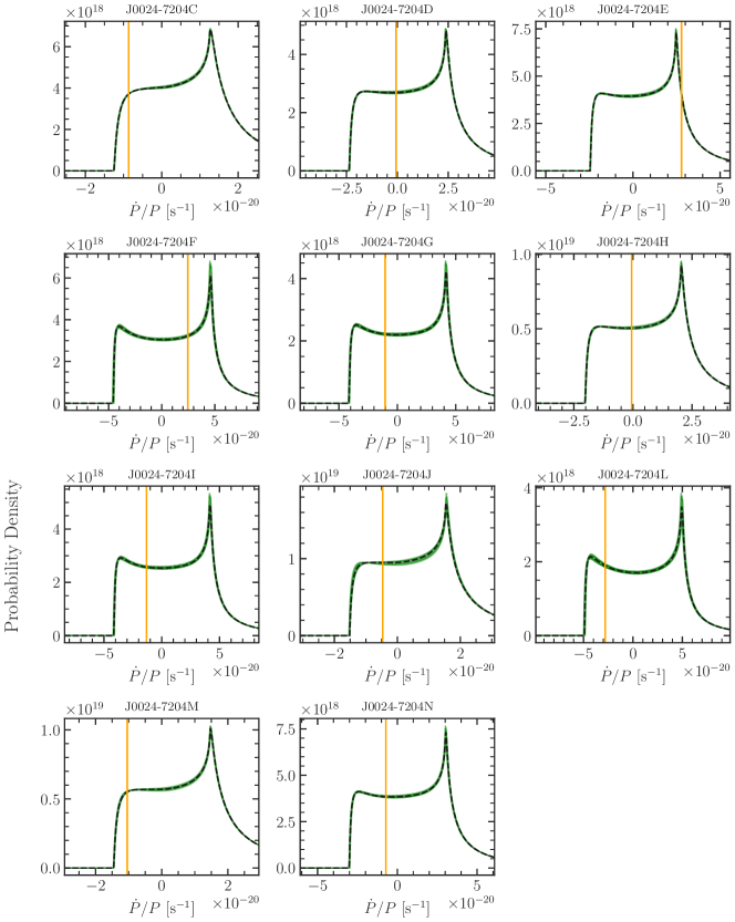
Figure 14: Likelihood functions corresponding to the best-fitting model (47Tuc-AllData) for the observed $\dot{P}/P$ for each pulsar in 47 Tuc. In each panel, we show the observed period derivative as a vertical orange line.

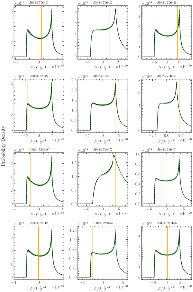
Figure 15: Continuation of Figure 14.

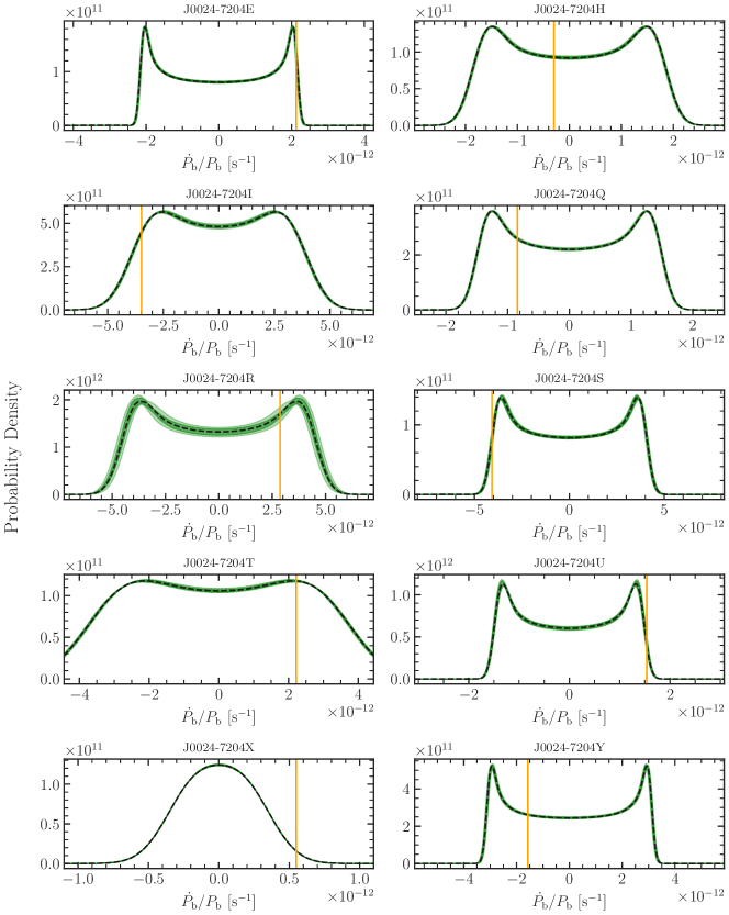
Figure 16: Likelihood functions corresponding to the best-fitting model (47Tuc-AllData) for the observed $\dot{P}_{\rm b}/P_{\rm b}$ for each pulsar in 47 Tuc with an orbital timing solution. In each panel, we show the observed period derivative as a vertical orange line.

The 47Tuc-NoPulsars fit is very similar to the fit presented in Dickson et al. (2024), and we use this fit as a baseline to evaluate the additional leverage provided by the pulsar data. The 47Tuc-AllData fit to all of the available data is shown in Figure 4 and Figure 5, along with examples of the likelihood functions for the measured pulsar period derivatives for the best-fitting models shown in Figure 6 (top panels) and all pulsars in Figures 14, 15 and 16.

Figure 4: Best-fitting model (in orange) for the 47Tuc-AllData fit compared to different datasets (in blue). Top left: Model fit to the projected number density profile. Top right: Model fit to the projected line-of-sight velocity dispersion profile. Bottom panels: Model fit to the projected proper motion dispersion profile, separated into radial (left panel) and tangential (right panel) components. The shaded regions represent the $1\sigma$ and $2\sigma$ credible intervals.

Figure 5: Continuation of Figure 4 showing the best-fitting model for the 47Tuc-AllData fit compared to the stellar mass function data of 47 Tuc. Each colour corresponds to a different HST field and each panel to a different radial region within a field. We display the HST proposal ID for in the first panel of each field.

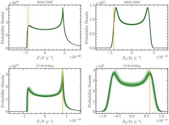
Figure 6: Likelihood functions corresponding to the best-fitting model for the observed $\dot{P}/P$ and $\dot{P}_{\rm b}/P_{\rm b}$ (recall that $P$ and $P_{\rm b}$ are the spin and orbital periods of the pulsars) for one pulsar in each cluster. Top left: The $\dot{P}/P$ likelihood for pulsar S in 47 Tuc from the 47Tuc-AllData fit. Top right: The $\dot{P}_{\rm b}/P_{\rm b}$ likelihood for pulsar S in 47 Tuc from the 47Tuc-AllData fit. Bottom left: The $\dot{P}/P$ likelihood for pulsar ap in Terzan 5 from the Ter5-AllData fit. Bottom right: The $\dot{P}_{\rm b}/P_{\rm b}$ likelihood for pulsar ap in Terzan 5 from the Ter5-AllData fit. In each panel, we show the observed period derivative as a vertical orange line. We show similar plots for all of the pulsars in Figures 14 through 19.

An initial comparison of the 47Tuc-AllData and 47Tuc-NoPulsars fits reveals no significant differences, either in model parameters, fit quality or derived quantities like the black hole mass fraction. We take this agreement as an indication that the 47Tuc-NoPulsars fit already provides a very good description of the underlying mass distribution and dynamics of the cluster, as probed by and fully consistent with the pulsar data.

Given the agreement between the 47Tuc-AllData and 47Tuc-NoPulsars fits, we turn to the third case in order to evaluate the leverage provided by the pulsar data. In the 47Tuc-NoKin fit we seek to emulate the data that we have for Terzan 5. For this fit, we fix the mass function to the bottom-light IMF of Baumgardt et al. (2023) discussed in Section 3.5. This mass function is a reasonable approximation for 47 Tuc and is similar to the best-fitting mass function we infer when the mass function is allowed to vary (see Table 3). We show part of the results for this third fit in Figure 7, where the best-fitting model is plotted along with the stellar kinematic data even though this data is excluded from the fit. This model is in excellent agreement with the data, similar to the models that are directly fit on the stellar kinematics and the best fit parameters for this fit are similar to the previous two fits (see Table 3). A comparison of the enclosed mass profiles of the 47Tuc-AllData and 47Tuc-NoKin fits reveal that the mass profiles vary by less than $\sim 15\%$ within the innermost $1\text{\,}\mathrm{p}\mathrm{c}$ (where the 47Tuc-NoKin fit contains less mass) and the total mass varies only by $\sim 5\%$ with the 47Tuc-NoKin fit favoring a slightly higher mass.

Figure 7: Same as Figure 4 but for the 47Tuc-NoKin fit. The best-fitting model is plotted along with the stellar kinematic data even though this data is excluded from the fit.

We show our inferred posterior probability distribution for the cluster mass in BHs for each of our three fits of 47 Tuc in Figure 8. While the results for the 47Tuc-AllData and 47Tuc-NoPulsars fits are quite similar and both resemble the results of Dickson et al. (2024), the 47Tuc-NoKin fit is worth discussing in more detail. The most obvious feature of this fit is that the posterior distribution of the mass in BHs is much broader than the cases with abundant stellar kinematic and mass function data, and this posterior is also not uni-modal. Despite this, we can still place a very stringent upper limit (99th percentile) on the mass in BHs, limiting this mass to less than $\sim 0.1\%$ of the total cluster mass, even in the 47Tuc-NoKin fit. Finally, the 47Tuc-AllData posterior shows non-zero probability as it approaches zero mass in BHs, indicating that with all data included, we cannot rule out the possibility that this cluster hosts zero BHs at the present day. We further note that even though we have adopted a fixed IMF for the 47Tuc-NoKin fit, the inferred BH content is consistent with the fits where we allow the IMF to vary.

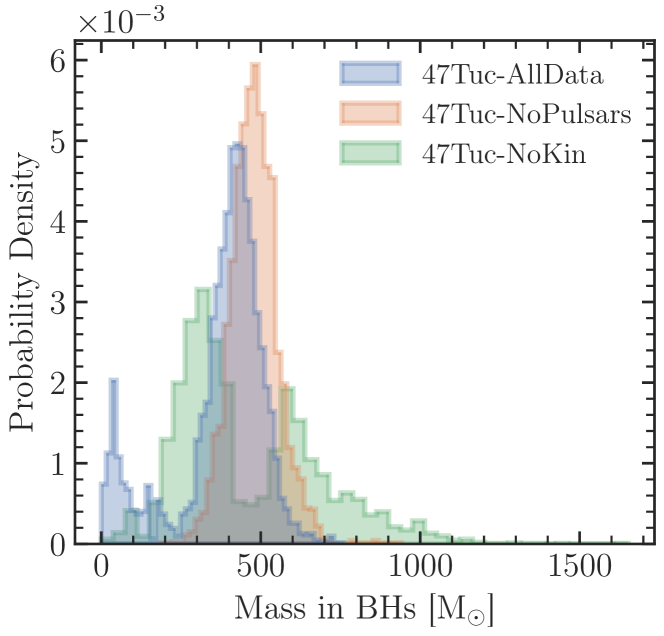
Figure 8: Posterior probability distribution of the mass in BHs in 47 Tuc for each of the fits summarized in Table 2.

These tests demonstrate that the pulsar timing data can provide constraints on the central dynamics, BH content, and mass distribution of the cluster very similar to the stellar kinematics, and in cases like Terzan 5 where the stellar kinematic data are lacking, pulsar timing data may provide an excellent substitute. With this in mind, we discuss the case of Terzan 5 next.

4.2 Terzan 5

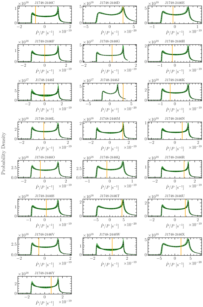
Figure 17: Likelihood functions corresponding to the best-fitting model (Ter5-AllData) for the observed $\dot{P}/P$ for each pulsar in Terzan 5. In each panel, we show the observed period derivative as a vertical orange line.

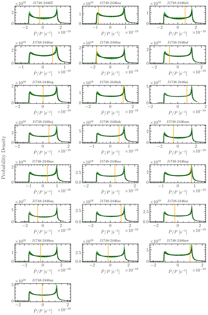
Figure 18: Continuation of Figure 17.

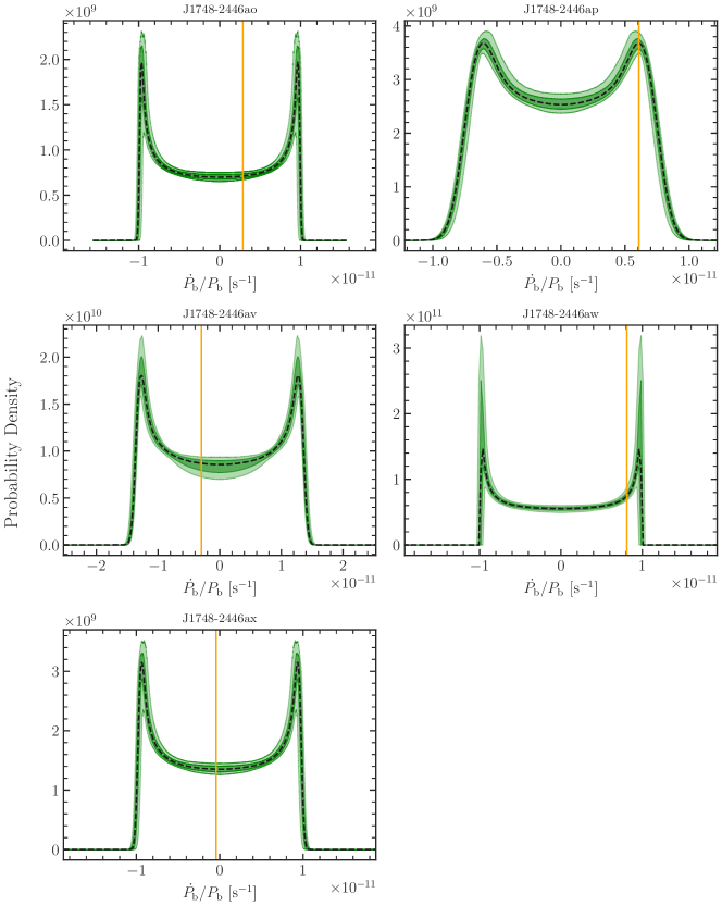
Figure 19: Likelihood functions corresponding to the best-fitting model (Ter5-AllData) for the observed $\dot{P}_{\rm b}/P_{\rm b}$ for each pulsar in Terzan 5 with an orbital timing solution. In each panel, we show the observed period derivative as a vertical orange line.

We show the Ter5-AllData fit in Figures 9 and 10, along with examples of the likelihood functions for the measured period derivatives for the best-fitting models shown in Figure 6 (bottom panels) and all the pulsars in Figures 17, 18 and 19. Our best-fitting model for the Ter5-AllData fit is in excellent agreement with the data and is able to fully reproduce all of the observables, including the pulsar data. The comparative lack of data for Terzan 5 means that our inferred model parameters for Terzan 5 generally have larger uncertainties compared to our fits of 47 Tuc. We present the median and $1\sigma$ uncertainties on all model parameters in Table 3.

Figure 9: Best-fitting model (in orange) for the Ter5-AllData fit compared to different datasets (in blue). Top left: Model fit to the projected number density profile. Top right: Model fit to the projected line-of-sight velocity dispersion profile. Bottom: Model fit to the projected proper motion dispersion profile. The shaded regions represent the $1\sigma$ and $2\sigma$ credible intervals of the model fits.

When we do not fit on the pulsar data (Ter5-NoPulsars), the uncertainties on model parameters and related quantities generally become larger than was the case for the Ter5-AllData fit. This comparison suggests that the pulsar data can play a more dominant role in constraining the models in the case of Terzan 5 (compared to 47 Tuc), given the lack of stellar kinematic data for this bulge cluster.

The third fit, Ter5-NoKinNoMF, was done to test the reliability of the stellar kinematics data given the challenge of membership determination in the Galactic bulge. As we find for 47 Tuc, even when we exclude the stellar kinematic data from the fit, the pulsar timing data provides enough constraints that the resulting best-fitting model is relatively similar and generally in good agreement with the held-out data. With the insight from 47 Tuc (see Section 4.1) that pulsars can provide strong constraints on the mass distribution of a cluster, we interpret this agreement as a sign that the existing stellar kinematics for Terzan 5, while sparse, are likely not suffering from significant contamination or other systematic effects.

As mentioned previously, the stellar mass function data available for Terzan 5 does not cover a wide enough range of masses or radii to a sufficient completeness level to allow us to leave the mass function slopes as free parameters when fitting models. We adopted the IMF of Baumgardt et al. (2023) for each of our three fits and we show in Figure 10 that this mass function is in excellent agreement with the available data.

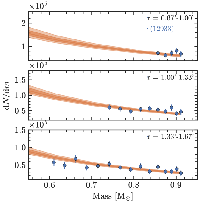
Figure 10: Continuation of Figure 9 showing the best-fitting model for the Ter5-AllData fit compared to the stellar mass function data of Terzan 5. Each panel corresponds to a different radial region within the HST field.

We show our inferred cluster masses in BHs for each of our fits of Terzan 5 in Figure 11. Comparing the fits, it is again obvious that the pulsar data is providing most of the constraining power, with the Ter5-NoPulsars fit resulting in an upper bound on the mass in BHs roughly double that of the two fits that do include the pulsar data. Even with the inclusion of the pulsar data we are only able to place an upper limit on the mass in BHs in this cluster, though we do significantly improve on existing estimates, lowering the range of allowed masses by a factor of $\sim 10$ (see discussion in Section 5.3). As was the case for 47 Tuc, we cannot rule out that Terzan 5 contains zero BHs at the present day and indeed our posterior distribution of mass in BHs is peaked towards zero for both fits that include the pulsar data.

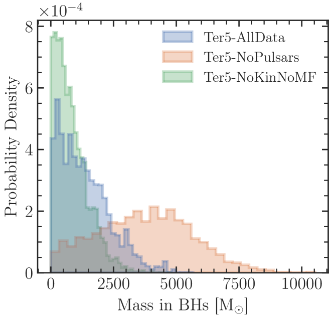
Figure 11: Posterior probability distribution of the mass in BHs in Terzan 5 for each of the fits summarized in Table 2.

5 Discussion

5.1 Constraints from pulsars

The specific constraints provided by the pulsar data are on the local acceleration of each pulsar, and thus on the enclosed mass profile of the cluster. The most stringent constraints come from pulsars with larger negative observed values of $\dot{P}/P$. This can be seen most easily in the rightmost panel of Figure 3 where the positive side of the $\dot{P}/P$ distribution has a long tail due to the convolution with the intrinsic spin-down distribution. By contrast, the negative side of the $\dot{P}/P$ distribution truncates sharply to zero at the $\dot{P}/P$ corresponding to the maximum possible acceleration at a given projected radius. In terms of specific pulsars, this means that pulsar S and aa in 47 Tuc provide the strictest limits on the enclosed mass while pulsar ae provides the strictest limits in Terzan 5. When inferring the dark remnant content of a cluster (in particular BHs), the ideal pulsars would be very close to the center of the cluster and would have large negative observed values of $\dot{P}/P$ , as these pulsars place the strongest constraints on the central mass distribution of their host cluster, where the mass density is dominated by heavy remnants due to mass segregation. We show in Figure 12 the minimum and maximum allowed values of $\dot{P}/P$ and $\dot{P}_{\rm b}/P_{\rm b}$ due to the cluster potential, where pulsars providing these stronger constraints fall along the bottom contour of the allowed values of $\dot{P}/P$.

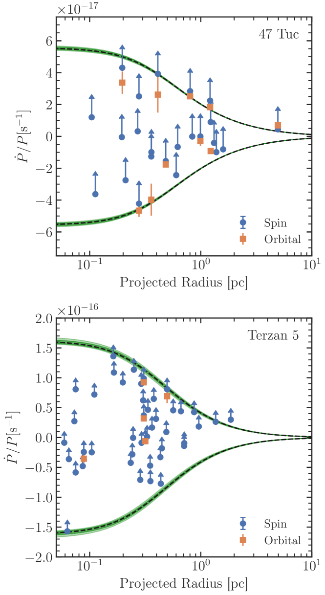
Figure 12: Minimum and maximum values of $\dot{P}/P$ allowed from the acceleration in the cluster potential for the best-fitting models of our 47Tuc-AllData (top) and Ter5-AllData (bottom) fits. We show the median values as a dashed line while the shaded regions represent the $1\sigma$ and $2\sigma$ credible intervals of the model fits. The observed $\dot{P}/P$ of the pulsars are shown with blue circles and the observed $\dot{P}_{\rm b}/P_{\rm b}$ are shown with orange squares. Uncertainties on the $\dot{P}_{\rm b}/P_{\rm b}$ points represent measurement errors while the upward-facing error bars on the $\dot{P}/P$ points show the typical width of the $\dot{P}_{\rm int}$ distribution at each pulsar’s location in the $P$-$\dot{P}$ plane shown in Figure 1. Note that pulsars above the maximum contour are not disallowed by our models due to the long tails on the spin-down side of the likelihood function shown in Figure 3. We note that we have converted the projected radius of each pulsar from angular to linear units using the median value of our inferred distances to each cluster from the AllData fits (see Table 3).

Our finding of pulsar S being the most constraining pulsar in 47 Tuc is not new and was discussed by Giersz & Heggie (2011). These authors reported that when attempting to find a suitable Monte Carlo model of 47 Tuc, the tension between the central surface brightness and the large negative acceleration of pulsar S was the single most impactful factor. Similarly, Figure 2 (extended) of Kızıltan et al. (2017a) shows that pulsar S is just barely compatible with their model and could potentially be a driving factor in requiring more mass in the cluster center, therefore favoring models with an IMBH. Pulsars 47Tuc-S and Ter5-ae do have a binary companions (Freire et al., 2017; Prager et al., 2017), however, due to the fact that the companions are low-mass WDs any spin-up effects from accretion which would shift the observed spin period derivatives towards more negative values are very unlikely. Pulsar 47Tuc-aa appears to be an isolated pulsar, leaving little possibility for accretion-induced spin-up. Because these pulsars are not likely to experience any spin period change from accretion, the constraints that their spin period derivatives place on the mass distribution of the cluster are likely trustworthy.

While pulsars with large negative observed values of $\dot{P}/P$ provide the strongest constraints, the majority of pulsars have values that are much closer to zero or even on the positive extreme of the distribution. These pulsars nonetheless provide useful constraints on the mass distribution of the cluster, particularly when it comes to constraining the total mass of the cluster. These pulsars have observed values of $\dot{P}/P$ that would be technically compatible with any model containing some minimum mass at their radius. As the mass of the model grows however, the range of possible $\dot{P}/P$ values grows, lowering the probability of observing these less extreme values. In this way the pulsars provide not just a minimum enclosed mass at their projected radius, but also some leverage on the exact value of the enclosed mass. We can see this when we compare our fits of Terzan 5 with different subsets of the data, as the best-fitting models found when including the pulsar data in the fits (Ter5-AllData and Ter5-NoKinNoMF) are less massive than the fit that excludes the pulsar data (Ter5-NoPulsars).

5.2 Mass of Terzan 5

The total mass of Terzan 5 is somewhat uncertain in the current literature, with mass estimates based on photometry (e.g. Lanzoni et al., 2010) a factor of a few higher than those based on kinematics and dynamical modeling (e.g. Baumgardt & Hilker, 2018; Prager et al., 2017). We show in Figure 13 our inferred cumulative mass profile along with several literature values for the cluster mass. Our profile is in good agreement with the estimate of the enclosed mass at $1\text{\,}\mathrm{p}\mathrm{c}$ from Prager et al. (2017) and our total mass estimate of $0.77\begin{subarray}{c}+0.08\\ -0.11\end{subarray}\times 10^{6}\ \mathrm{M}_{\odot}$ is in good agreement with the total masses of Baumgardt & Hilker (2018) and Baumgardt et al. (2019a) given that the true uncertainty on our inferred mass from multimass modeling is likely closer to $10\%$ (see Section 3 in Dickson et al., 2024). The masses inferred from kinematics and dynamical modeling, including our own value, are a factor of $2-3$ times smaller than the mass inferred by Lanzoni et al. (2010) from photometry. A lower present-day mass for Terzan 5 potentially has many important implications, in particular for studies that seek to model the star-formation and chemical enrichment histories of this system (e.g. Romano et al., 2023).

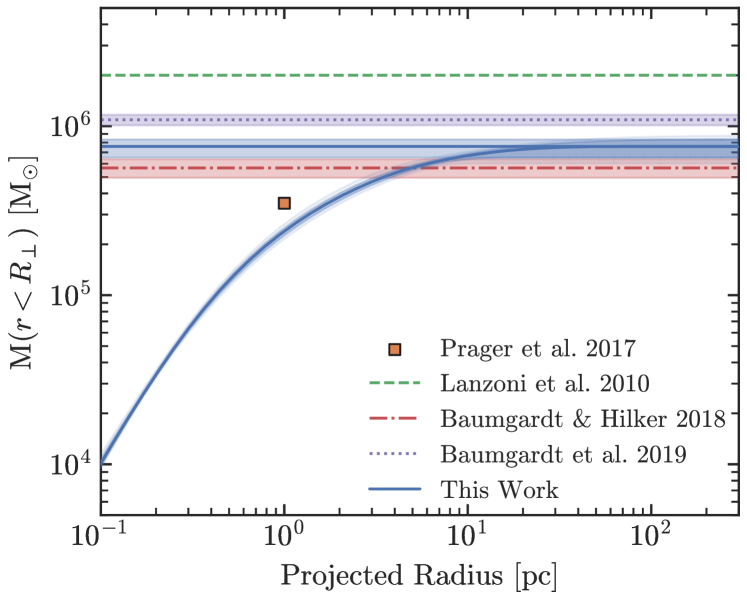
Figure 13: The inferred cumulative mass profile of Terzan 5 from our Ter5-AllData fit. We show the median values as a solid line (blue) while the shaded regions represent the $1\sigma$ and $2\sigma$ credible intervals of the model fit. The enclosed mass at $1\text{\,}\mathrm{p}\mathrm{c}$ measured by Prager et al. (2017) is shown with an orange square. We show our inferred total mass and the values from Lanzoni et al. (2010), Baumgardt & Hilker (2018) and Baumgardt et al. (2019a) as horizontal dashed lines where the shaded regions represent the $1\sigma$ credible intervals.

5.3 Comparison of mass in BHs to literature results

Our models allow us to place strong constraints on the mass in BHs in both 47 Tuc and Terzan 5. We compare our results with other studies that investigate the BH population in these clusters in Table 4.

47 Tuc is a well-studied cluster with many previous works investigating its BH content, using a variety of methods. In general, we see that recent works which employ Monte Carlo models (Weatherford et al., 2020; Ye et al., 2022) generally infer larger BH populations (with larger uncertainties) despite taking very different approaches while works employing equilibrium models favor somewhat smaller populations of BHs. Our models place an upper limit (99th percentile) on the total mass in BHs in 47 Tuc of $618\ \mathrm{M}_{\odot}$, very similar the results of Dickson et al. (2024) who did not consider pulsar timing data. Our results are also in very good agreement with the upper limit of $578\ \mathrm{M}_{\odot}$ on the mass of a central IMBH reported by Della Croce et al. (2024). These authors employ action-based distribution function models to derive an upper limit on the mass of a putative IMBH in 47 Tuc, which as discussed earlier (see discussion in Section 1), is expected to have similar dynamical effects to a compact central cluster of BHs. Our inferred upper limit on the mass in BHs corresponds to an upper limit of $0.07\%$ on the BH mass fraction $f_{\mathrm{BH}}$, slightly lower than the upper limit of $0.09\%$ found by Della Croce et al. (2024). These upper limits significantly limit the room for a more massive potential IMBH in 47 Tuc, which we discuss in the following section.

Terzan 5 on the other hand, has only a single estimate of its BH content reported in the literature, by Prager et al. (2017). These authors, also fitting on pulsar data, test for the presence of an IMBH in the center of 47 Tuc, reporting marginal evidence of a $\sim 500\ \mathrm{M}_{\odot}$ IMBH and an upper limit of . Our posterior for the mass in BHs in Terzan 5 is peaked near zero and the 99th percentile upper limit is $4437\ \mathrm{M}_{\odot}$ ($f_{\mathrm{BH}}<0.59\%$), representing an improvement of nearly one order of magnitude on the existing constraints on the mass in BHs.

Table 4: Reported masses in BHs (or upper limits) in 47 Tuc and Terzan 5 from dynamical studies in the literature and from this work. Note that we have scaled the BH mass fraction reported by Weatherford et al. (2020) to our inferred total mass to facilitate comparison. We note that the uncertainties on the black hole content reported by studies that employ limepy models (Hénault-Brunet et al. 2020; Dickson et al. 2024 and this work) are likely underestimated by a factor of $2-3$ (see discussion in Dickson et al. 2024). Listed uncertainties correspond to the $1\sigma$ uncertainties.

Study	47 Tuc	Terzan 5
Hénault-Brunet et al. (2020)	$430\begin{subarray}{c}+386\\ -301\end{subarray}\ \mathrm{M}_{\odot}$
Weatherford et al. (2020)	$1059\begin{subarray}{c}+1674\\ -941\end{subarray}\ \mathrm{M}_{\odot}$
Ye et al. (2022)	$\sim 2375\ \mathrm{M}_{\odot}$
Della Croce et al. (2024)	$<578\ \mathrm{M}_{\odot}$
Dickson et al. (2024)	$420\begin{subarray}{c}+150\\ -80\end{subarray}\ \mathrm{M}_{\odot}$
This work	$412\begin{subarray}{c}+77\\ -146\end{subarray}\ \mathrm{M}_{\odot}$	$<4437\ \mathrm{M}_{\odot}$
Prager et al. (2017)		$<30\,000\ \mathrm{M}_{\odot}$

5.4 An IMBH in 47 Tuc?

GCs have long been suggested to host IMBHs. For proposed detections in multiple clusters using various techniques, see e.g. Gerssen et al. (2002), Noyola et al. (2008), Jalali et al. (2012), Lützgendorf et al. (2015), Kamann et al. (2016), Baumgardt (2017), Kızıltan et al. (2017a), Paduano et al. (2024), and Häberle et al. (2024). Many of these possible detections have however been contested. Typically, follow-up studies find that the dynamical effects of a central IMBH and other ingredients like a large population of centrally concentrated dark stellar remnants (including stellar-mass black holes - BHs) are highly degenerate, making the detection of a non-accreting IMBH very difficult (see e.g. McNamara et al., 2003; Van Der Marel & Anderson, 2010; Freire et al., 2017; Zocchi et al., 2017, 2019; Gieles et al., 2018; Baumgardt et al., 2019c; Mann et al., 2019, 2020; Hénault-Brunet et al., 2020). Ruling out the presence of an IMBH is also very difficult, with most works placing only an upper limit on the dark mass in the core of a cluster (e.g. Mann et al., 2019; Häberle et al., 2021; Della Croce et al., 2024). Häberle et al. (2024) find seven stars with velocities above the inferred escape velocity in the inner 0.08 pc of $\omega$ Cen, and they conclude that this implies an IMBH with a mass $\gtrsim 8200\,\mathrm{M}_{\odot}$. We note that only two of those seven stars are above the escape velocity of the mass model of Dickson et al. (2023), but they are the two closest to the cluster center and remain difficult to reconcile with explanations other than an IMBH, making this the strongest case for an IMBH in a Galactic GC so far.

Particularly relevant to this work are the results from Kızıltan et al. (2017a, b) and Paduano et al. (2024) who each report evidence for an IMBH in 47 Tuc. Kızıltan et al. (2017a) reported evidence for a $2300\ \mathrm{M}_{\odot}$ IMBH in the center of 47 Tuc on the basis of pulsar timing measurements. In order to constrain the mass of a central IMBH, they compared snapshots from a grid of $N$-body models (with and without an IMBH) to surface density and velocity dispersion profiles. The best-fitting models with and without an IMBH were then compared to measurements of pulsar accelerations (based on period derivatives) due to the cluster’s gravitational potential, and the set of models with a central IMBH was found to be more consistent with these measurements.

Critically, several follow-up studies identified limitations and possible issues with the analysis of Kızıltan et al. (2017a) (see Freire et al. 2017; Mann et al. 2019, 2020; Hénault-Brunet et al. 2020). Among the issues raised was the assumption of a short cluster distance of $4\text{\,}\mathrm{k}\mathrm{p}\mathrm{c}$, the lack of primordial binaries in their $N$-body models, and the use of a grid of isolated $N$-body models that have a much steeper present-day mass function than the bottom-light mass function that is observed for 47 Tuc, all of which could affect the inferred amount of dark mass in the cluster core.

We note that models of 47 Tuc that do not include a central IMBH have been shown to satisfyingly reproduce its velocity dispersion profile, number density profile, and stellar mass function data (Baumgardt et al., 2019b; Hénault-Brunet et al., 2020; Dickson et al., 2023, 2024). These studies, however, either did not consider the pulsar data, or they checked that the models were consistent with the pulsars’ maximum accelerations and projected radial distribution but did not directly incorporate the pulsar timing data in the fitting process.

Our results allow us to address the claims of Kızıltan et al. (2017a) since we are directly fitting our models to the pulsar timing data. As mentioned previously, our fit to all the available 47 Tuc data (47Tuc-AllData) yields an upper limit of $618\ \mathrm{M}_{\odot}$ in BHs ($\sim 0.07\%$ of the total cluster mass). This argues against the conclusions of Kızıltan et al. (2017a) that the pulsar data requires a central IMBH of $2300\ \mathrm{M}_{\odot}$ to explain the observed values of $\dot{P}/P$. We performed a fit of 47 Tuc with the distance set to $4\text{\,}\mathrm{k}\mathrm{p}\mathrm{c}$, resulting in a noticeably worse quality of fit but also a larger ($\sim 1700\ \mathrm{M}_{\odot}$) population of BHs, perhaps indicating that the low distance assumed by Kızıltan et al. (2017a) contributes to the differences in our inferred dark mass in 47 Tuc.

The potential IMBH detection reported by Paduano et al. (2024) has a much wider range of possible masses, with the nominal 1$\sigma$ uncertainty range spanning $56-6000\ \mathrm{M}_{\odot}$. The results of Della Croce et al. (2024), who infer an upper limit on the mass of an IMBH in 47 Tuc of $578\ \mathrm{M}_{\odot}$ reduce this range substantially. The fact that our inferred upper limit on the mass in BHs is consistent with the upper limit on the mass of an IMBH from Della Croce et al. (2024) highlights the fact there is very little room for a significant dark mass in the center of 47 Tuc.

While the effects of an IMBH and a centrally concentrated population of BHs are expected to be similar, they are not identical because the dark mass is more centrally concentrated if it is in an IMBH. This means that an upper limit on the mass in BHs does not necessarily correspond directly to the upper limit on the mass of an IMBH. Despite this, we expect that in our models, these effects are likely degenerate due to the spatial regions probed by our datasets. The half-mass radius of the BH population in our 47Tuc-AllData fit is $\sim 0.1\ \mathrm{pc}$, which is more centrally concentrated than the majority of the pulsars in this cluster. While we do have a few pulsars inside this radius, the pulsars with large negative period derivatives (those that provide the most stringent constraints on the enclosed mass) are located outside of this radius meaning we are largely insensitive to the spatial extent and concentration of the mass in BHs in the central regions of the cluster.

We note that given the central line-of-sight velocity dispersion of 47 Tuc, the radius of influence of an IMBH of $\sim 600\ \mathrm{M}_{\odot}$ is $\lesssim 0.02\ \mathrm{pc}$ which at the distance of 47 Tuc corresponds to $\lesssim 0.8^{\prime\prime}$, a much smaller region than is probed by either the pulsar data or the stellar kinematic data. This means that any future work seeking to use stellar kinematics to understand the nature of the dark mass in the core of this cluster would need to precisely measure the velocities of individual stars in the central arcsecond of 47 Tuc.

5.5 Central velocity dispersion of Terzan 5

The existing stellar kinematic data for Terzan 5 does not probe the central regions of the cluster, but the pulsar timing data allows us to independently predict the central velocity distribution of bright stars, without directly relying on any stellar kinematics. This also allows us to validate the existing observed stellar kinematics for a cluster like Terzan 5 where bulge contamination makes membership selection especially difficult. Our predicted central dispersion for Terzan 5 based on fit Ter5-NoKinNoMF is $15.6\begin{subarray}{c}+0.4\\ -0.4\end{subarray}\ \textrm{km s}^{-1}$. Future work seeking to constrain the central kinematics of this cluster can use this prediction as a benchmark to which new measurements can be compared. For example, a cusp in the central velocity dispersion within the radius of influence of an IMBH should manifest as a velocity dispersion larger than this predicted central velocity dispersion given that our models do not contain an IMBH.

5.6 Terzan 5: a comparison with $\omega$ Cen

The formation of Terzan 5 and its multiple populations is a topic of much debate in the literature, with suggested formation channels ranging from the stripped core of an accreted dwarf galaxy (Ferraro et al., 2009, 2016) to a surviving fragment of the proto-bulge (Ferraro et al., 2009, 2016; Taylor et al., 2022) to the product of a collision between a typical GC and a giant molecular cloud or young massive cluster (McKenzie & Bekki, 2018; Pfeffer et al., 2021; Bastian & Pfeffer, 2022).

While it is generally accepted that the metal-rich population in Terzan 5 is too enriched to have formed in a low-mass dwarf galaxy (e.g. Bastian & Pfeffer, 2022), we can further investigate the dynamical evolution of this object by comparing Terzan 5 to $\omega$ Cen, a well-studied GC which is frequently suggested to be the core of an accreted dwarf galaxy (e.g. Pfeffer et al., 2021). $\omega$ Cen is the most massive GC in the Milky Way (e.g. Harris, 1996, 2010 edition) and hosts multiple stellar populations with a large spread in iron abundance (e.g. Johnson & Pilachowski, 2010; Bellini et al., 2017). Several studies have presented dynamical models of $\omega$ Cen which suggest that the cluster is host to a very large population of black holes (e.g. Zocchi et al., 2019; Baumgardt et al., 2019c; Dickson et al., 2024) typically making up about $5\%$ of the total cluster mass (consistent with having retained almost all its BHs). The fact that we infer a much smaller population of BHs and indeed rule out a population larger than $0.6\%$ of the total cluster mass in Terzan 5 suggests a different evolutionary history for this object. We note that $\omega$ Cen is more massive than Terzan 5 by a factor of $\sim 3-4$, and has a factor of $\sim 3$ larger $r_{\rm h}$, which both contribute to a higher retention of BHs by the present day for $\omega$ Cen through an order of magnitude longer relaxation time (diminishing the importance of dynamical ejections of BHs throughout the evolution of the cluster). Additionally, the higher metallicity of Terzan 5 compared to $\omega$ Cen is expected to produce lower-mass BHs from the same initial progenitor masses (e.g. Fryer et al., 2012; Banerjee et al., 2020), increasing the number of BHs lost to natal kicks and reducing the fraction of the cluster mass in BHs resulting from a given IMF.

While the origin of Terzan 5 remains uncertain, the discussion above highlights that further studies of the evolution of Terzan 5 along with its BH population could help to shed light on the initial conditions and formation of this peculiar system.

6 Conclusions

In this work, we presented a method to directly fit multimass dynamical models of GCs to pulsar timing data, allowing to infer the mass distribution of clusters. We applied our method to 47 Tuc, a well-studied cluster with a wealth of conventional stellar kinematic and local stellar mass function data as well as a large population of pulsars. We use this cluster as a benchmark by which we evaluate the performance of our method. We then applied our method to Terzan 5, a bulge cluster host to the largest population of pulsars of any Milky Way GC and lacking in conventional stellar kinematic data. Our main conclusions are as follows:

1. For clusters like 47 Tuc and Terzan 5 that are host to large populations of pulsars, the timing solutions of these pulsars can place similar constraints on the mass distribution and dynamics of their host cluster as conventional stellar kinematics. We demonstrate that the pulsar timing data allows us to accurately predict held-out stellar kinematic data and place strong constraints on the BH content of clusters.

2. We infer new and improved values for the mass and structural parameters of Terzan 5, finding a total mass of $0.77\begin{subarray}{c}+0.08\\ -0.11\end{subarray}\times 10^{6}\ \mathrm{M}_{\odot}$, and a (3D) half-mass radius of $2.7\begin{subarray}{c}+0.6\\ -0.7\end{subarray}\ \mathrm{pc}$. This mass is consistent with other dynamical estimates but is smaller by a factor of $2-3$ than the estimate derived from photometry.

3. We refine existing constraints on the BH content of 47 Tuc and lower the existing upper limit on the mass in BHs of Terzan 5 by an order of magnitude. We infer the presence of $412\begin{subarray}{c}+77\\ -146\end{subarray}\ \mathrm{M}_{\odot}$ in BHs in 47 Tuc and place an upper limit on the mass in BHs in Terzan 5 of $4437\ \mathrm{M}_{\odot}$.

4. Our results do not support the $\sim 2300\ \mathrm{M}_{\odot}$ IMBH reported by Kızıltan et al. (2017a) in the center of 47 Tuc on the basis of pulsar timing data, as we instead infer an upper limit of $618\ \mathrm{M}_{\odot}$ in BHs in this cluster, representing $\sim 0.07\%$ of the total cluster mass. This adds to several follow-up studies that refuted this original claim, but it is the first time that pulsar timing data, a crucial component of the Kızıltan et al. (2017a) study, is revisited as a direct constraint on the dynamical models.

5. We predict the central velocity dispersion of Terzan 5, independently of any stellar kinematic data, finding a dispersion of $15.6\begin{subarray}{c}+0.4\\ -0.4\end{subarray}\ \mathrm{km\ s^{-1}}$. This prediction provides a baseline to which future work seeking to measure the central kinematics of this cluster can be compared.

The next generation of radio telescopes is expected to dramatically increase the number of detected pulsars in GCs (e.g. Hessels et al., 2015; Ridolfi et al., 2021; Chen et al., 2023; Berteaud et al., 2024), allowing us to apply our methodology to clusters that are not currently known to host large numbers of pulsars.

Perhaps the most promising candidate to host a large number of undiscovered pulsars is Liller 1, a bulge cluster that is qualitatively very similar to Terzan 5 (e.g. Ferraro et al., 2021). Liller 1 is a massive cluster ($\sim 1\times 10^{6}\ \mathrm{M}_{\odot}$, Baumgardt et al. 2019a) that is similarly compact to Terzan 5 and has been found to have a similarly high stellar encounter rate (Saracino et al., 2015). This high stellar encounter rate, combined with strong gamma-ray emission detected from this cluster, suggests that it may be host to hundreds of undiscovered MSPs (Tam et al., 2011).

Like Terzan 5, Liller 1 is difficult to observe due to its location, with bulge contamination and strong differential reddening (e.g. Pallanca et al., 2021) making the collection of conventional stellar kinematic data very difficult. As we have shown for Terzan 5, pulsars present a unique opportunity to investigate the internal dynamics of even heavily obscured clusters.

Appendix A Supplementary Material

A.1 Incorporating dispersion measures

Given a description of the gas distribution within a cluster (e.g. Abbate et al., 2018) Equation 6 can be modified to use the dispersion measure of a pulsar to form the line-of-sight probability distribution instead of using the model line-of-sight density profile:

$$P\left(a_{{\rm cl},z}\mid R_{i}\right)\propto\frac{\mathrm{d}m}{\mathrm{d}a_{{\rm cl},z}}=\frac{\mathrm{d}m}{\mathrm{d}z}\absolutevalue{\frac{\mathrm{d}z}{\mathrm{d}a_{{\rm cl},z}}}=\frac{P\left(z\mid z_{{\rm DM},i},\sigma_{z,{\rm DM},i}\right)}{\left|\frac{\mathrm{d}a_{{\rm cl},z}}{\mathrm{d}z}\right|},$$ (A1)

where we have replaced the $\frac{\mathrm{d}m}{\mathrm{d}z}$ term with $P\left(z\mid z_{\rm DM},\sigma_{z,{\rm DM}}\right)$, the probability distribution of line-of-sight positions $z$ given the predicted line-of-sight position from the dispersion measure $z_{\rm DM}$ and its uncertainty $\sigma_{z,{\rm DM}}$. The values of $z_{{\rm DM},i}$ and $\sigma_{z,{\rm DM}}$ can be calculated from the an individual dispersion measure $\mathrm{DM}_{i}$, $n_{g}$ and $\mathrm{DM_{c}}$ as $z_{{\rm DM},i}=({\rm DM}_{i}-{\rm DM_{c}})/n_{g}$ (under the assumption of a uniform gas distribution) with $\sigma_{z,{\rm DM}}$ following from Gaussian error propagation. $P\left(z\mid z_{{\rm DM},i},\sigma_{z,{\rm DM},i}\right)$ is then a Gaussian probability density function, centered at $z_{{\rm DM},i}$ with a dispersion of $\sigma_{z,{\rm DM}}$:

$$P\left(z\mid z_{{\rm DM},i},\sigma_{z,{\rm DM},i}\right)=\frac{1}{\sigma_{z,{\rm DM},i}\sqrt{2\pi}}\exp\left(-\frac{1}{2}\left(\frac{z-z_{{\rm DM},i}}{\sigma_{z,{\rm DM},i}}\right)^{\!2}\,\right).$$ (A2)

A.2 Pulsar Data

Table 5: Pulsar timing data used in this work for 47 Tuc. The columns indicate the pulsar ID, projected radius, spin period, spin-period derivative, the uncertainty on the spin-period derivative, the orbital period, the orbital period derivative and the uncertainty on the orbital period derivative. In the rightmost column we indicate the work in which the timing solution was derived. Timing References: F17: Freire et al. (2017), R16: Ridolfi et al. (2016), FR18: Freire & Ridolfi (2018).

Pulsar ID	$R$ [’]	$P$ [ms]	$\dot{P}$ [s/s]	$\Delta\dot{P}$ [s/s]	$P_{\rm b}$ [days]	$\dot{P}_{\rm b}$ [s/s]	$\Delta\dot{P}_{\rm b}$ [s/s]	Timing Reference
J0024-7204C	1.2298	5.75678	-4.99e-20	2e-24	–	–	–	F17
J0024-7204D	0.6483	5.35757	-3.42e-21	9e-25	–	–	–	F17
J0024-7204E	0.6205	3.53633	9.85e-20	5e-25	2.2568483	4.8e-12	2e-13	F17
J0024-7204F	0.2149	2.62358	6.45e-20	7e-25	–	–	–	F17
J0024-7204G	0.2781	4.04038	-4.22e-20	2e-24	–	–	–	F17
J0024-7204H	0.7677	3.21034	-1.83e-21	1e-24	2.357696895	-7e-13	6e-13	F17
J0024-7204I	0.2772	3.48499	-4.59e-20	2e-24	0.2297922489	-8e-13	2e-13	F17
J0024-7204J	1.0185	2.10063	-9.79e-21	9e-25	–	–	–	F17
J0024-7204L	0.1627	4.34617	-1.22e-19	1e-24	–	–	–	F17
J0024-7204M	1.0688	3.67664	-3.84e-20	5e-24	–	–	–	F17
J0024-7204N	0.4793	3.05395	-2.19e-20	2e-24	–	–	–	F17
J0024-7204O	0.0806	2.64334	3.03e-20	6e-25	–	–	–	F17
J0024-7204Q	0.9502	4.03318	3.4e-20	6e-25	1.1890840496	-1e-12	2e-13	F17
J0024-7204R	0.1519	3.48046	1.48e-19	3e-24	0.06623147751	1.9e-13	4e-14	F17
J0024-7204S	0.215	2.83041	-1.21e-19	1e-24	1.2017242354	-4.9e-12	4e-13	F17
J0024-7204T	0.3179	7.58848	2.94e-19	1e-23	1.126176771	2.5e-12	1.1e-12	F17
J0024-7204U	0.9386	4.34283	9.52e-20	2e-24	0.42910568324	6.6e-13	5e-14	F17
J0024-7204W	0.087	2.35234	-8.66e-20	1e-24	–	–	–	R16
J0024-7204X	3.828	4.77152	1.84e-20	7e-25	10.921183545	6e-12	2e-12	R16
J0024-7204Y	0.3743	2.19666	-3.52e-20	8e-25	0.5219386107	-8.2e-13	7e-14	F17
J0024-7204Z	0.1506	4.55445	-4.56e-21	1e-22	–	–	–	F17
J0024-7204aa	0.465	1.84538	-4.59e-20	1.5e-23	–	–	–	FR18
J0024-7204ab	0.2092	3.70464	9.82e-21	8e-24	–	–	–	F17

Table 6: Same as Table 5 but for Terzan 5. Timing References: L00: Lyne et al. (2000), R05: Ransom et al. (2005), P17: Prager et al. (2017), C18: Cadelano et al. (2018), A18: Andersen & Ransom (2018), R21: Ridolfi et al. (2021), P24: Padmanabh et al. (2024).

Pulsar ID	$R$ [’]	$P$ [ms]	$\dot{P}$ [s/s]	$\Delta\dot{P}$ [s/s]	$P_{\rm b}$ [days]	$\dot{P}_{\rm b}$ [s/s]	$\Delta\dot{P}_{\rm b}$ [s/s]	Timing Reference
J1748-2446C	0.179	8.4361	-6.06e-19	4e-21	–	–	–	L00
J1748-2446D	0.693	4.71398	1.3e-19	–	–	–	–	R05
J1748-2446E	0.361	2.1978	-1.8e-20	–	–	–	–	R05
J1748-2446F	0.125	5.54014	4e-21	–	–	–	–	R05
J1748-2446G	0.185	21.6719	3.9e-19	–	–	–	–	R05
J1748-2446H	0.227	4.92589	-8.3e-20	–	–	–	–	R05
J1748-2446I	0.03	9.57019	-7.1e-20	–	–	–	–	R05
J1748-2446J	0.948	80.3379	2.5e-18	–	–	–	–	R05
J1748-2446K	0.22	2.96965	-9.4e-20	–	–	–	–	R05
J1748-2446L	0.149	2.2447	-1.7e-20	–	–	–	–	R05
J1748-2446M	0.083	3.56957	4.9e-19	–	–	–	–	R05
J1748-2446N	0.154	8.6669	5.5e-19	–	–	–	–	R05
J1748-2446O	0.119	1.67663	-6.9e-20	–	–	–	–	R05
J1748-2446Q	0.36	2.812	-3.6e-20	–	–	–	–	R05
J1748-2446R	0.101	5.02854	4.7e-19	–	–	–	–	R05
J1748-2446S	0.249	6.11664	6.4e-20	–	–	–	–	R05
J1748-2446T	0.443	7.08491	3.1e-19	–	–	–	–	R05
J1748-2446U	0.148	3.28914	3e-19	–	–	–	–	R05
J1748-2446V	0.178	2.07251	-9.5e-20	–	–	–	–	R05
J1748-2446W	0.037	4.20518	1.2e-19	–	–	–	–	R05
J1748-2446X	0.488	2.99926	5.9e-20	–	–	–	–	R05
J1748-2446Y	0.056	2.04816	1.5e-19	–	–	–	–	R05
J1748-2446Z	0.033	2.46259	-8.6e-20	–	–	–	–	P17
J1748-2446aa	0.222	5.78804	-4.4e-19	–	–	–	–	P17
J1748-2446ab	0.038	5.11971	4.2e-19	–	–	–	–	P17
J1748-2446ac	0.337	5.08691	2.3e-19	–	–	–	–	P17
J1748-2446ae	0.032	3.65859	-5.7e-19	–	–	–	–	P17
J1748-2446af	0.145	3.30434	-2.3e-19	–	–	–	–	P17
J1748-2446ag	0.167	4.44803	1.2e-20	–	–	–	–	P17
J1748-2446ah	0.127	4.96515	5.7e-19	–	–	–	–	P17
J1748-2446ai	0.192	21.22838	1.4e-18	–	–	–	–	P17
J1748-2446aj	0.17	2.95891	1.41232e-19	6e-24	–	–	–	C18
J1748-2446ak	0.287	1.8901	8.8495e-20	6-24	–	–	–	C18
J1748-2446am	0.044	2.93382	-1.368e-19	3e-23	–	–	–	A18
J1748-2446an	0.201	4.802	1.55746e-19	6-24	–	–	–	R21
J1748-2446ao	0.156	2.27438	8.6979e-20	1e-24	57.5556	1.65e-10	9e-12	P24
J1748-2446ap	0.253	3.74469	3.07e-19	1e-24	21.3882	1.3e-10	2.1e-11	P24
J1748-2446aq	0.038	12.52194	-7.16198e-19	6e-24	–	–	–	P24
J1748-2446as	0.084	2.32646	2.559829e-19	6e-25	–	–	–	P24
J1748-2446at	0.123	2.18819	-5.89966e-20	4e-25	–	–	–	P24
J1748-2446au	0.053	4.54822	-1.06797e-19	2e-24	–	–	–	P24
J1748-2446av	0.045	1.84945	-4.25047e-20	2e-25	3.38166	-1e-11	2e-12	P24
J1748-2446aw	0.156	13.04908	1.306465e-18	3e-24	0.73138	5.92e-12	2e-14	P24
J1748-2446ax	0.161	1.9435	-9.5495e-21	7e-25	30.2088	-1.3e-11	9e-12	P24

A.3 Supplementary Figures

References

- Abbate et al. (2019a) Abbate, F., Possenti, A., Colpi, M., & Spera, M. 2019a, The Astrophysical Journal, 884, L9, doi: 10.3847/2041-8213/ab46c3
- Abbate et al. (2018) Abbate, F., Possenti, A., Ridolfi, A., et al. 2018, Monthly Notices of the Royal Astronomical Society, 481, 627, doi: 10.1093/mnras/sty2298
- Abbate et al. (2019b) Abbate, F., Spera, M., & Colpi, M. 2019b, Monthly Notices of the Royal Astronomical Society, 487, 769, doi: 10.1093/mnras/stz1330
- Andersen & Ransom (2018) Andersen, B. C., & Ransom, S. M. 2018, The Astrophysical Journal, 863, L13, doi: 10.3847/2041-8213/aad59f
- Aros & Vesperini (2023) Aros, F. I., & Vesperini, E. 2023, Monthly Notices of the Royal Astronomical Society, 525, 3136, doi: 10.1093/mnras/stad2429
- Bacon et al. (2010) Bacon, R., Accardo, M., Adjali, L., et al. 2010, SPIE Proceedings, 7735, 773508, doi: 10.1117/12.856027
- Balbinot & Gieles (2018) Balbinot, E., & Gieles, M. 2018, Monthly Notices of the Royal Astronomical Society, 474, 2479, doi: 10.1093/mnras/stx2708
- Banerjee et al. (2020) Banerjee, S., Belczynski, K., Fryer, C. L., et al. 2020, Astronomy & Astrophysics, 639, A41, doi: 10.1051/0004-6361/201935332
- Bastian & Pfeffer (2022) Bastian, N., & Pfeffer, J. 2022, Monthly Notices of the Royal Astronomical Society, 509, 614, doi: 10.1093/mnras/stab3081
- Baumgardt (2017) Baumgardt, H. 2017, Monthly Notices of the Royal Astronomical Society, 464, 2174, doi: 10.1093/mnras/stw2488
- Baumgardt et al. (2023) Baumgardt, H., Hénault-Brunet, V., Dickson, N., & Sollima, A. 2023, Monthly Notices of the Royal Astronomical Society, 521, 3991, doi: 10.1093/mnras/stad631
- Baumgardt & Hilker (2018) Baumgardt, H., & Hilker, M. 2018, Monthly Notices of the Royal Astronomical Society, 478, 1520, doi: 10.1093/mnras/sty1057
- Baumgardt et al. (2019a) Baumgardt, H., Hilker, M., Sollima, A., & Bellini, A. 2019a, Monthly Notices of the Royal Astronomical Society, 482, 5138, doi: 10.1093/mnras/sty2997
- Baumgardt et al. (2019b) Baumgardt, H., Sollima, A., & Hilker, M. 2019b, Proceedings of the International Astronomical Union, 14, 400, doi: 10.1017/S1743921319007695
- Baumgardt & Vasiliev (2021) Baumgardt, H., & Vasiliev, E. 2021, Monthly Notices of the Royal Astronomical Society, 505, 5957, doi: 10.1093/mnras/stab1474
- Baumgardt et al. (2019c) Baumgardt, H., He, C., Sweet, S. M., et al. 2019c, Monthly Notices of the Royal Astronomical Society, 488, 5340, doi: 10.1093/mnras/stz2060
- Bellini et al. (2017) Bellini, A., Milone, A. P., Anderson, J., et al. 2017, The Astrophysical Journal, 844, 164, doi: 10.3847/1538-4357/aa7b7e
- Berteaud et al. (2024) Berteaud, J., Eckner, C., Calore, F., Clavel, M., & Haggard, D. 2024, Simulation-Based Inference of Radio Millisecond Pulsars in Globular Clusters, arXiv. https://arxiv.org/abs/2405.15691
- Binney & Tremaine (2008) Binney, J., & Tremaine, S. 2008, Galactic Dynamics (Princeton University Press)
- Blandford et al. (1987) Blandford, R. D., Romani, R. W., & Applegate, J. H. 1987, Monthly Notices of the Royal Astronomical Society, 225, 51p, doi: 10.1093/mnras/225.1.51P
- Bovy (2015) Bovy, J. 2015, The Astrophysical Journal Supplement Series, 216, 29, doi: 10.1088/0067-0049/216/2/29
- Cadelano et al. (2018) Cadelano, M., Ransom, S. M., Freire, P. C. C., et al. 2018, The Astrophysical Journal, 855, 125, doi: 10.3847/1538-4357/aaac2a
- Chen et al. (2023) Chen, W., Freire, P. C. C., Ridolfi, A., et al. 2023, Monthly Notices of the Royal Astronomical Society, 520, 3847, doi: 10.1093/mnras/stad029
- Claydon et al. (2019) Claydon, I., Gieles, M., Varri, A. L., Heggie, D. C., & Zocchi, A. 2019, Monthly Notices of the Royal Astronomical Society, 487, 147, doi: 10.1093/mnras/stz1109
- De Boer et al. (2019) De Boer, T. J., Gieles, M., Balbinot, E., et al. 2019, Monthly Notices of the Royal Astronomical Society, 485, 4906, doi: 10.1093/mnras/stz651
- Della Croce et al. (2024) Della Croce, A., Pascale, R., Giunchi, E., et al. 2024, Astronomy and Astrophysics, 682, A22, doi: 10.1051/0004-6361/202347569
- Dickson et al. (2023) Dickson, N., Hénault-Brunet, V., Baumgardt, H., Gieles, M., & Smith, P. J. 2023, Monthly Notices of the Royal Astronomical Society, 522, 5320, doi: 10.1093/mnras/stad1254
- Dickson et al. (2024) Dickson, N., Smith, P. J., Hénault-Brunet, V., Gieles, M., & Baumgardt, H. 2024, Monthly Notices of the Royal Astronomical Society, 529, 331, doi: 10.1093/mnras/stae470
- Ferraro et al. (2016) Ferraro, F. R., Massari, D., Dalessandro, E., et al. 2016, The Astrophysical Journal, 828, 75, doi: 10.3847/0004-637X/828/2/75
- Ferraro et al. (2009) Ferraro, F. R., Dalessandro, E., Mucciarelli, A., et al. 2009, Nature, 462, 483, doi: 10.1038/nature08581
- Ferraro et al. (2021) Ferraro, F. R., Pallanca, C., Lanzoni, B., et al. 2021, Nature Astronomy, 5, 311, doi: 10.1038/s41550-020-01267-y
- Foreman-Mackey et al. (2013) Foreman-Mackey, D., Hogg, D. W., Lang, D., & Goodman, J. 2013, Publications of the Astronomical Society of the Pacific, 125, 306, doi: 10.1086/670067
- Foreman-Mackey et al. (2019) Foreman-Mackey, D., Farr, W., Sinha, M., et al. 2019, Journal of Open Source Software, 4, 1864, doi: 10.21105/joss.01864
- Freire & Ridolfi (2018) Freire, P. C., & Ridolfi, A. 2018, Monthly Notices of the Royal Astronomical Society, 476, 4794, doi: 10.1093/mnras/sty524
- Freire et al. (2017) Freire, P. C., Ridolfi, A., Kramer, M., et al. 2017, Monthly Notices of the Royal Astronomical Society, 471, 857, doi: 10.1093/MNRAS/STX1533
- Fryer et al. (2012) Fryer, C. L., Belczynski, K., Wiktorowicz, G., et al. 2012, Astrophysical Journal, 749, 91, doi: 10.1088/0004-637X/749/1/91
- Gerssen et al. (2002) Gerssen, J., van der Marel, R. P., Gebhardt, K., et al. 2002, The Astronomical Journal, 124, 3270, doi: 10.1086/344584
- Gieles et al. (2018) Gieles, M., Balbinot, E., Yaaqib, R. I. S. M., et al. 2018, Monthly Notices of the Royal Astronomical Society, 473, 4832, doi: 10.1093/mnras/stx2694
- Gieles & Zocchi (2015) Gieles, M., & Zocchi, A. 2015, Monthly Notices of the Royal Astronomical Society, 454, 576, doi: 10.1093/mnras/stv1848
- Giersz & Heggie (2011) Giersz, M., & Heggie, D. C. 2011, Monthly Notices of the Royal Astronomical Society, 410, 2698, doi: 10.1111/j.1365-2966.2010.17648.x
- Gill et al. (2008) Gill, M., Trenti, M., Miller, M. C., et al. 2008, The Astrophysical Journal, 686, 303, doi: 10.1086/591269
- Häberle et al. (2021) Häberle, M., Libralato, M., Bellini, A., et al. 2021, Monthly Notices of the Royal Astronomical Society, 503, 1490, doi: 10.1093/mnras/stab474
- Häberle et al. (2024) Häberle, M., Neumayer, N., Seth, A., et al. 2024, Fast-Moving Stars around an Intermediate-Mass Black Hole in Omega Centauri, arXiv. https://arxiv.org/abs/2405.06015
- Harris et al. (2020) Harris, C. R., Millman, K. J., van der Walt, S. J., et al. 2020, Nature, 585, 357, doi: 10.1038/s41586-020-2649-2
- Harris (1996) Harris, W. E. 1996, The Astronomical Journal, 112, 1487, doi: 10.1086/118116
- Hénault-Brunet et al. (2019) Hénault-Brunet, V., Gieles, M., Sollima, A., et al. 2019, Monthly Notices of the Royal Astronomical Society, 483, 1400, doi: 10.1093/mnras/sty3187