Distilling circularly polarized photon emission from magnetized chiral plasmas

Abstract

We investigate the emission of circularly polarized photons from a magnetized quark-gluon plasma with nonzero quark-number and chiral charge chemical potentials. These chemical potentials qualitatively influence the differential emission rates of circularly polarized photons. A nonzero net electric charge density, induced by quark-number chemical potentials, enhances the overall emission of one circular polarization over the other, while a nonzero chiral charge density introduces a spatial asymmetry in the emission with respect to reflection in the transverse plane. The signs of the electrical and chiral charge densities determine which circular polarization dominates overall and whether the emission preferentially aligns with or opposes the magnetic field. Based on these findings, we propose that polarized photon emission is a promising observable for characterizing the quark-gluon plasma produced in heavy-ion collisions.

I Introduction

Over the past two decades, the study of exotic states of matter in extreme environments has become a central focus of modern nuclear physics. This interest is largely driven by successful experimental programs at the relativistic heavy-ion colliders in Brookhaven and CERN. The ultrarelativistic collisions produce quark-gluon plasma (QGP) at temperatures well above the quark deconfinement transition. By analyzing particle spectra and correlations, one uncovers valuable information about the fundamental properties of QGP.

High temperature and energy density are not the only extreme characteristics of the QGP produced by heavy-ion collisions. The system is, without exaggeration, rich in extremes. Since heavy ions carry electric charges, they induce extreme magnetic fields [1, 2, 3, 4, 5]. Furthermore, large values of angular momentum in non-central collisions can produce high vorticity in the resulting QGP fluid [6, 7]. Many theoretical aspects of QGP associated with strong magnetic fields and high vorticity are routinely tested in experimental studies [8, 9, 10, 11]. (For reviews, see Refs. [12, 13, 14, 15, 16].)

One aspect we would like to discuss in more detail is the effect of chiral charge density on the electromagnetic probes of QGP. A nonzero chiral charge arises from an imbalance between left-handed and right-handed quarks in the plasma. At first glance, such a state may seem too exotic as it would break local parity symmetry. However, in a hot plasma, local bubbles of chiral plasma can be produced by topological configurations of gauge fields [17]. This idea is not new, and it is taken seriously enough to motivate the challenging search for its observable signatures via the dipole and quadrupole chiral magnetic effects (CME) in multiple experiments. Unfortunately, the evidence supporting CME remains inconclusive.

This study was motivated by the proposition that there might be unexplored, better observables for detecting chiral plasma effects. Electromagnetic probes, such as photon and dilepton emissions, play a crucial role in revealing the properties of QGP in strong magnetic fields. These probes provide valuable information about temperature, magnetic fields, flow characteristics, and possibly much more. Naturally, one might ask how a nonzero chiral charge affects electromagnetic probes. Some attempts to address this question have been made before, see Ref. [18, 19, 20]. Here, we delve into more detail to illuminate the role of strong magnetic fields and propose new observables that may resolve the issue. While the task remains challenging, we believe it is not impossible.

This paper is organized as follows. In Sec. II, we briefly present the formalism used for studying polarized photon emission from the plasma. Numerical results for the polarized photon emission are given in Sec. III. In Sec. IV, we discuss our main findings and summarize the results. Several technical derivations and auxiliary results are provided in the appendices at the end of the paper.

II Formalism

To investigate the impact of a nonzero chiral charge density on photon emission from a strongly magnetized plasma, we will utilize the general framework developed in Refs. [21, 22]. Specifically, we will utilize a relationship between the emission rate and the imaginary part of the retarded photon polarization tensor [23]

$${\cal R}_{\rm diff}\equiv k^{0}\frac{d^{3}R}{dk_{x}dk_{y}dk_{z}}=-\frac{1}{(2\pi)^{3}}\frac{\mbox{Im}\left[g^{\mu\nu}\Pi_{\mu\nu}(k)\right]}{\exp\left(\frac{k_{0}}{T}\right)-1}.$$ (1)

Assuming that the background magnetic field is sufficiently strong, the polarization tensor $\Pi_{\mu\nu}(k)$ is determined by the simplest one-loop diagram at the leading order of coupling [22]. For QED plasma, this approximation should hold true for magnetic field strengths $|eB|\gtrsim\alpha T^{2}$, where $\alpha=1/137$ denotes the fine structure constant. In the context of QGP, the requirement is $|eB|\gtrsim\alpha_{s}T^{2}$, where $\alpha_{s}$ is the strong coupling constant. Additionally, in the case of QCD, one should require that $T\gg\Lambda_{\rm QCD}$.

To separate total emission into polarized components, we use the following completeness relation:

$$g^{\mu\nu}=\epsilon_{0}^{\mu}\epsilon_{0}^{\nu*}-\epsilon_{+}^{\mu}\epsilon_{+}^{\nu*}-\epsilon_{-}^{\mu}\epsilon_{-}^{\nu*}-\epsilon_{\parallel}^{\mu}\epsilon_{\parallel}^{\nu*}.$$ (2)

where $\epsilon_{r}^{\mu}$ are photon polarization vectors. Here, we will use the same basis for $\epsilon_{r}^{\mu}$ as in Refs. [19, 20], i.e., $\epsilon_{0}^{\mu}=(1,0,0,0)$, $\epsilon_{\parallel}^{\mu}=(0,0,0,1)$, $\epsilon_{\pm}^{\mu}=(0,1,\pm i,0)/\sqrt{2}$. (A slightly different decomposition was used in the study of dilepton production in Ref. [24].)

This study focuses on the emission of circularly polarized photons, represented by the polarization vectors $\epsilon_{\pm}^{\mu}$. Before proceeding further, it is important to clarify the exact physical meaning of these photon states. For emission along (or opposite to) the direction of the magnetic field, these states correspond to the left-handed and right-handed circular polarizations, or equivalently, photons with positive and negative helicities, respectively. For photons emitted in other directions in the upper and lower hemispheres, they serve only as proxies for representing photons with given circular polarizations. For our qualitative discussion, we ignore the subtle difference between true circular polarization and its proxy defined by $\epsilon_{\pm}^{\mu}$. This is acceptable since, from symmetry considerations, both characterize closely related photon emission observables.

Note that the projection operators for circularly polarized photons take the following explicit form:

$$\epsilon_{\pm}^{\mu}\epsilon_{\pm}^{\nu*}=(-g_{\perp}^{\mu\nu}\pm i\epsilon_{\perp}^{\mu\nu})/2,$$ (3)

where $g_{\perp}^{\mu\nu}=g^{\mu\nu}-\delta^{\mu}_{0}\delta^{\nu}_{0}$ and $\epsilon_{\perp}^{\mu\nu}=\delta^{\mu}_{1}\delta^{\nu}_{2}-\delta^{\mu}_{2}\delta^{\nu}_{1}$. For completeness, let us note that the projectors for the other two states are $\epsilon_{0}^{\mu}\epsilon_{0}^{\nu*}=\mbox{diag}(1,0,0,0)$ and $\epsilon_{\parallel}^{\mu}\epsilon_{\parallel}^{\nu*}=\mbox{diag}(0,0,0,1)$. When these projectors are contracted with $\Pi_{\mu\nu}(k)$, as in Eq. (1), the photon polarization tensor naturally separates into the following four parts:

$$g^{\mu\nu}\Pi_{\mu\nu}(k)\to\Pi^{(0)}(k)+\Pi^{(+)}(k)+\Pi^{(-)}(k)+\Pi^{(\parallel)}(k).\$$ (4)

Then, the emission rate in Eq. (1) similarly splits into four parts. It is natural to interpret the contributions proportional to $\mbox{Im}\left[\Pi^{(+)}(k)\right]$ and $\mbox{Im}\left[\Pi^{(-)}(k)\right]$,

$${\cal R}^{(+)}_{\rm diff} \equiv k^{0}\frac{d^{3}R}{dk_{x}dk_{y}dk_{z}}=-\frac{1}{(2\pi)^{3}}\frac{\mbox{Im}\left[\Pi^{(+)}(k)\right]}{\exp\left(\frac{k_{0}}{T}\right)-1},$$ (5)

$${\cal R}^{(-)}_{\rm diff} \equiv k^{0}\frac{d^{3}R}{dk_{x}dk_{y}dk_{z}}=-\frac{1}{(2\pi)^{3}}\frac{\mbox{Im}\left[\Pi^{(-)}(k)\right]}{\exp\left(\frac{k_{0}}{T}\right)-1},$$ (6)

as the emission rates for photons with the right-handed and the left-handed circular polarizations, respectively. It is important to emphasize, however, that such an interpretation is not entirely correct.

Recall that photons have only two physical degrees of freedom. Nevertheless, in the conventional quantum field theoretical description of a gauge theory like QED, it is convenient to introduce four states. Two of these states are unphysical. While they ensure the gauge invariance of the theory, they should not affect physical observables such as the photon emission rate. Thus, if all physical contributions were included in ${\cal R}^{(+)}_{\rm diff}$ and ${\cal R}^{(-)}_{\rm diff}$, the remaining parts would cancel out. However, this is not the case, partly due to the use of approximate rather than exact definitions of the polarization projectors in Eq. (3).

Interestingly, the extra contribution ${\cal R}^{\rm(extra)}_{\rm diff}$ to the rate, coming from $\Pi^{\rm(extra)}(k)\equiv\Pi^{(0)}(k)+\Pi^{(\parallel)}(k)$, is negative. This may seem problematic since the rates are expected to be positive definite. However, as one can verify, the total rate ${\cal R}^{\rm(extra)}_{\rm diff}$ is always positive. This implies that the extra contribution ${\cal R}^{\rm(extra)}_{\rm diff}$ should be distributed between the two physical circular polarizations, modifying the definitions of rates in Eqs. (5) and (6). For simplicity, we will use the unmodified definitions above, which should suffice to approximately extract parity-odd contributions (albeit somewhat overestimated) to the rates for circularly polarized photons.

To calculate $\Pi_{\mu\nu}(k)$ in the QGP, we will assume that the plasma is made of the lightest up and down quarks. Their flavor-dependent quark charges are $e_{f}=eq_{f}$, where $f=u,d$, $q_{u}=2/3$, $q_{d}=-1/3$, and $e$ is the absolute value of the electron charge. When investigating the role of the chiral chemical potential $\mu_{5}$, it is convenient to use the chiral limit for quarks by setting their masses to zero. Noting that typical temperatures of a deconfined QGP are of the order of $200~{}\mbox{MeV}$ or higher and the current quark masses are only about $5~{}\mbox{MeV}$, the chiral limit is a very good approximation for the purposes of our study.

Without loss of generality, we will take the background magnetic field $\mathbf{B}$ to be along the $+z$ direction. In the Dirac equation for the quarks, it will be described by a vector potential in the Landau gauge, i.e., $\mathbf{A}=(-By,0,0)$. The corresponding quark Green’s functions $G_{f}(u,u^{\prime})$ take the form of a product of the so-called Schwinger phase $e^{i\Phi(u,u^{\prime})}$ and a translation invariant function $\bar{G}_{f}(u-u^{\prime})$, where $u=(t,x,y,z)$. Note, however, that the Schwinger phase plays no role in the calculation of the polarization tensor $\Pi_{\mu\nu}(k)$ in the leading one-loop order approximation [22].

In a mixed coordinate-momentum space representation, the Fourier transform of the translation invariant part of Green’s function can be conveniently given as a sum over the Landau levels [15]

$$\bar{G}_{f}(p_{0},p_{z};\mathbf{r}_{\perp})=i\frac{e^{-\mathbf{r}_{\perp}^{2}/(4\ell_{f}^{2})}}{2\pi\ell_{f}^{2}}\sum_{n=0}^{\infty}\frac{\tilde{D}_{n}^{f}(p_{0},p_{z};\mathbf{r}_{\perp})}{\mathcal{M}-2n|e_{f}B|}.$$ (7)

where the function in the numerator has the following explicit form:

$$\tilde{D}_{n}^{f}(p_{0},p_{z};\mathbf{r}_{\perp})=\left[(p_{0}+\mu)\gamma^{0}-p_{z}\gamma^{3}-\mu_{5}\gamma^{0}\gamma^{5}\right]\left[\mathcal{P}_{+}^{f}L_{n}\left(\frac{\mathbf{r}_{\perp}^{2}}{2\ell_{f}^{2}}\right)+\mathcal{P}_{-}^{f}L_{n-1}\left(\frac{\mathbf{r}_{\perp}^{2}}{2\ell_{f}^{2}}\right)\right]-\frac{i}{\ell_{f}^{2}}(\mathbf{r}_{\perp}\cdot\bm{\gamma}_{\perp})L_{n-1}^{1}\left(\frac{\mathbf{r}_{\perp}^{2}}{2\ell_{f}^{2}}\right).$$ (8)

Here, $L_{n}^{\alpha}(z)$ are the generalized Laguerre polynomials [25], $\mathcal{P}_{\pm}^{f}\equiv\frac{1}{2}\left(1\pm is_{\perp}\gamma^{1}\gamma^{2}\right)$ are the spin projectors, $\mathbf{r}_{\perp}=(x,y)$ is the transverse position vector, and $\ell_{f}=1/\sqrt{|e_{f}B|}$ is the magnetic length. Here, we included a nonzero quark number and chiral chemical potentials, denoted by $\mu$ and $\mu_{5}$, respectively. By definition, $s_{\perp}=\,\mbox{sign}(e_{f}B)$ and $L_{-1}^{\alpha}(z)\equiv 0$.

The function in the denominator of Eq. (7) is a Dirac matrix. In the chiral limit, the corresponding fraction takes the following form:

$$\frac{1}{\mathcal{M}-2n|e_{f}B|}=\frac{\mathcal{P}_{5}^{(-)}}{(p_{0}+\mu+\mu_{5})^{2}-2n|e_{f}B|-p_{z}^{2}}+\frac{\mathcal{P}_{5}^{(+)}}{(p_{0}+\mu-\mu_{5})^{2}-2n|e_{f}B|-p_{z}^{2}},$$ (9)

where $\mathcal{P}_{5}^{(\pm)}=\frac{1}{2}(1\pm\gamma^{5})$ are the chirality projectors. Note that we included both the quark-number and chiral-charge chemical potentials, $\mu$ and $\mu_{5}$, respectively. Both play important role in polarized photon emission. For the sake of simplicity, we assume that $\mu$ and $\mu_{5}$ are same for both flavors. (The generalization to the case of flavor-dependent chemical potentials is straightforward and will be briefly discussed later.)

By using the above Green’s functions in the Landau-level representation, we derive the following formal expression for the polarization tensor [22]:

$$\Pi^{\mu\nu}(i\Omega_{m};\mathbf{k})=4\pi\sum_{f=u,d}N_{c}\alpha_{f}T\sum_{k=-\infty}^{\infty}\int\frac{dp_{z}}{2\pi}\int d^{2}\mathbf{r}_{\perp}e^{-i\mathbf{r}_{\perp}\cdot\mathbf{k}_{\perp}}\,\mbox{tr}\left[\gamma^{\mu}\bar{G}_{f}(i\omega_{k},p_{z};\mathbf{r}_{\perp})\gamma^{\nu}\bar{G}_{f}(i\omega_{k}-i\Omega_{m},p_{z}-k_{z};-\mathbf{r}_{\perp})\right],$$ (10)

where we used the Matsubara finite-temperature formalism. By definition, the fermionic and bosonic Matsubara frequencies are $\omega_{k}=(2k+1)\pi T$ and $\Omega_{m}=2n\pi T$, respectively. Regarding other notations, $\alpha_{f}=q_{f}^{2}\alpha$ is the flavor-dependent coupling constant, and $N_{c}=3$ is the number of quark colors.

By substituting Green’s function (7) into the definition for $\Pi^{\mu\nu}(i\Omega_{m};\mathbf{k})$, calculating the Dirac traces, integrating over $r_{\perp}$ and performing the Matsubara summation, we derive the following expression for the components of the polarization tensor:

$$\Pi^{(i)}(i\Omega_{m};\mathbf{k})=-\sum_{f=u,d}\frac{N_{c}\alpha_{f}}{\pi\ell_{f}^{4}}\sum_{n,n^{\prime}=0}^{\infty}\sum_{s,\eta,\lambda=\pm 1}\int\frac{dp_{z}}{2\pi}\frac{[n_{F}(E_{n,p_{z},f}+\eta\mu+\eta s\mu_{5})-n_{F}(\lambda E_{n^{\prime},p_{z}-k_{z},f}+\eta\mu+\eta s\mu_{5})]\mathcal{F}^{(i)}_{s,f}(\xi,i\Omega_{m})}{4\lambda E_{n,p_{z},f}E_{n^{\prime},p_{z}-k_{z},f}\left[E_{n,p_{z},f}-\lambda E_{n^{\prime},p_{z}-k_{z},f}+i\eta\Omega_{m}\right]},$$ (11)

where $i$ labels the photon polarizations (i.e., $i=0,+,-,\parallel$), $E_{n,p_{z},f}=\sqrt{p_{z}^{2}+2n|e_{f}B|}$ are Landau-level energies, and $n_{F}(E)=1/\left[\exp(E/T)+1\right]$ is the Fermi-Dirac distribution function. The corresponding technical details of the derivation are given in Appendices A, B, C, and D. The explicit forms of the polarization-dependent functions $\mathcal{F}^{(i)}_{s,f}(\xi,i\Omega_{m})$ are presented in Eqs. (40) – (43) in Appendix E.

After replacing $i\Omega_{m}\rightarrow k_{0}+i\epsilon$, it is straightforward to extract the absorptive part of the individual polarization component functions,

$$\mbox{Im}\Pi^{(i)}(k_{0};\mathbf{k}) = \sum_{f=u,d}\frac{N_{c}\alpha_{f}}{4\pi\ell_{f}^{4}}\sum_{s,s^{\prime}=\pm 1}\sum_{n>n^{\prime}}^{\infty}\frac{g(n,n^{\prime})\,\theta\left[(k_{-}^{f})^{2}+k_{z}^{2}-k_{0}^{2}\right]}{\sqrt{\left[(k_{-}^{f})^{2}+k_{z}^{2}-k_{0}^{2}\right]\left[(k_{+}^{f})^{2}+k_{z}^{2}-k_{0}^{2}\right]}}\left.\mathcal{F}^{(i)}_{s,f}(\xi,k_{0})\right|_{p_{z}=p_{z,f}^{(s^{\prime})}}$$ (12)

$$+ \sum_{f=u,d}\frac{N_{c}\alpha_{f}}{4\pi\ell_{f}^{4}}\sum_{s,s^{\prime}=\pm 1}\sum_{n<n^{\prime}}^{\infty}\frac{g(n,n^{\prime})\,\theta\left[(k_{-}^{f})^{2}+k_{z}^{2}-k_{0}^{2}\right]}{\sqrt{\left[(k_{-}^{f})^{2}+k_{z}^{2}-k_{0}^{2}\right]\left[(k_{+}^{f})^{2}+k_{z}^{2}-k_{0}^{2}\right]}}\left.\mathcal{F}^{(i)}_{s,f}(\xi,k_{0})\right|_{p_{z}=p_{z,f}^{(s^{\prime})}}$$

$$- \sum_{f=u,d}\frac{N_{c}\alpha_{f}}{4\pi\ell_{f}^{4}}\sum_{s,s^{\prime}=\pm 1}\sum_{n,n^{\prime}=0}^{\infty}\frac{g(n,n^{\prime})\,\theta\left[k_{0}^{2}-k_{z}^{2}-(k_{+}^{f})^{2}\right]}{\sqrt{\left[k_{0}^{2}-k_{z}^{2}-(k_{-}^{f})^{2}\right]\left[k_{0}^{2}-k_{z}^{2}-(k_{+}^{f})^{2}\right]}}\left.\mathcal{F}^{(i)}_{s,f}(\xi,k_{0})\right|_{p_{z}=p_{z,f}^{(s^{\prime})}},$$

where $\theta(x)$ is the Heaviside step function. In Eq. (12), we also introduced two transverse momentum thresholds,

$$k_{\pm}^{f}=\left|\sqrt{2n|e_{f}B|}\pm\sqrt{2n^{\prime}|e_{f}B|}\right|.$$ (13)

and the following function:

$$g(n,n^{\prime})=1-\sum_{s_{1}=\pm 1}n_{F}\left(\left[\frac{k_{0}}{2}+s_{1}\frac{k_{0}(n-n^{\prime})|e_{f}B|}{k_{0}^{2}-k_{z}^{2}}+s_{1}s^{\prime}\frac{|k_{z}|}{2}\sqrt{\left(1-\frac{(k_{-}^{f})^{2}}{k_{0}^{2}-k_{z}^{2}}\right)\left(1-\frac{(k_{+}^{f})^{2}}{k_{0}^{2}-k_{z}^{2}}\right)}\right]-s_{1}\mu-s_{1}s\mu_{5}\right).\\$$ (14)

Note that the photon energy $k_{0}$ in the final expression satisfies the mass-shell condition, i.e., $k_{0}=\sqrt{k_{\perp}^{2}+k_{z}^{2}}$.

As expected, the expression in Eq. (12) closely resembles the result in Ref. [22]. It should be noted, however, that $g(n,n^{\prime})$ depends on both fermion-number and chiral chemical potentials. The most important difference appears in the definition of functions $\mathcal{F}^{(i)}_{s,f}(\xi,\Omega)|_{p_{z}=p_{z,f}^{(s^{\prime})}}$, which define individual polarization components labeled by $i=0,+,-,\parallel$. Their explicit expressions are given in Eqs. (49) – (52) in Appendix E.

III Numerical results

Here, we present the main numerical results for the emission rates of circularly polarized photons. Considering potential applications to heavy-ion phenomenology, we will rewrite the differential rate using new variables:

$${\cal R}^{(\pm)}_{\rm diff}(k_{T},\phi,y)=\frac{d^{3}R^{(\pm)}}{k_{T}dk_{T}d\phi dy},$$ (15)

where we introduced the transverse momentum $k_{T}$, the azimuthal angle $\phi$, and the rapidity $y$, replacing the Cartesian components of the momentum, $k_{x}$, $k_{y}$, and $k_{z}$. By definition, $k_{y}=k_{T}\cos\phi$, $k_{z}=k_{T}\sin\phi$, and $y=\frac{1}{2}\ln\frac{k_{0}+k_{x}}{k_{0}-k_{x}}$. For simplicity, below we will be presenting the results for $y=0$ (i.e., $k_{x}=0$).

In calculating the imaginary part of the polarization tensor, defined by Eq. (12), we must sum over all Landau levels. For the numerical calculation, we will truncate the sum at a finite number of terms, specifically $n_{\rm max}=500$. This large number of Landau levels ensures high accuracy of the results across a wide range of model parameters.

For this study, we need to calculate the differential emission rate over the entire range of azimuthal angles, from $\phi_{\rm min}=-\pi/2$ to $\phi_{\rm max}=\pi/2$. To achieve high angular resolution, we use a relatively small step size, $\delta\phi=\pi/600$.

Our goal is to identify qualitative features of polarized photon emission in the presence of nonzero chemical potentials $\mu$ and $\mu_{5}$. Therefore, we limit our numerical analysis to a few representative values of the model parameters. Specifically, we consider two different values of the magnetic field strength, $|eB|=m_{\pi}^{2}$ and $|eB|=5m_{\pi}^{2}$, and two different values of temperature, $T=200~{}\mbox{MeV}$ and $T=350~{}\mbox{MeV}$.

III.1 Nonzero quark-number chemical potential $\mu$

Let us begin with the case of a nonzero quark-number chemical potential $\mu$. For our analysis, we will use a representative value of $\mu=200~{}\mbox{MeV}$. It is important to note that using the same chemical potential for both quark flavors implies that the plasma is positively charged overall, due to the up quark’s charge being twice as large in magnitude compared to the down quark’s charge. This analysis can be easily generalized to cases with different chemical potentials for the up and down quarks. As we argue below, it is the sign of the charge carriers in the plasma that determines the dominance of one circular polarization over the other in photon emission.

Typical numerical results for the emission rates of left-handed and right-handed circularly polarized photons are presented in Fig. 1. The data is shown for $T=350~{}\mbox{MeV}$ and two different values of the magnetic field, $|eB|=m_{\pi}^{2}$ and $|eB|=5m_{\pi}^{2}$, in the left and right panels, respectively. We verified that the qualitative features at $T=200~{}\mbox{MeV}$ are similar, though the rates are overall lower.

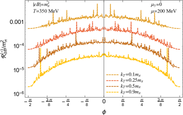
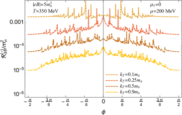
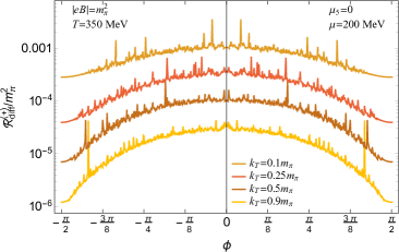
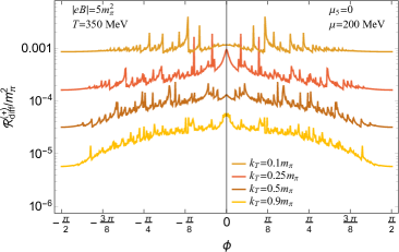
Figure 1: The angular dependence of left-handed (top) and right-handed (bottom) circularly polarized photon emission for two magnetic fields, $|eB|=m_{\pi}^{2}$ (left) and $|eB|=5m_{\pi}^{2}$ (right). The plasma temperature is $T=350~{}\mbox{MeV}$.

Each panel in Fig. 1 shows the differential rates for four different fixed values of the transverse momentum, $k_{T}=0.1m_{\pi},~{}0.25m_{\pi},~{}0.5m_{\pi},~{}0.9m_{\pi}$. Note that the transverse momentum also coincides with the photon energy since we set the rapidity to zero, $y=0$. The two top and two bottom panels display the results for left-handed and right-handed circular polarizations, respectively. As seen from the figure, the rates for both polarizations are symmetric under changing $\phi\to-\phi$, which is equivalent to reflection in the transverse plane.

We observe, however, that the emission rates for left-handed and right-handed circular polarizations differ significantly, with the latter being a few times larger than the former. To quantify this effect, it is instructive to calculate the degree of circular polarization, defined by

$${\cal P}_{\rm circ}(k_{T},\phi,y)=\frac{{\cal R}^{(+)}_{\rm diff}(k_{T},\phi,y)-{\cal R}^{(-)}_{\rm diff}(k_{T},\phi,y)}{{\cal R}^{(+)}_{\rm diff}(k_{T},\phi,y)+{\cal R}^{(-)}_{\rm diff}(k_{T},\phi,y)}.$$ (16)

The corresponding numerical results are presented in Fig. 2, which confirm a substantial degree of circular polarization in the photon emission. This sign of ${\cal P}_{\rm circ}(k_{T},\phi,y)$ is determined primarily by a nonzero electrical charge density in the plasma. Indeed, by separating the partial contributions from the up and down quarks, we find that the up quarks emit more left-handed photons (${\cal P}^{\rm(u)}_{\rm circ}<0$), while the down quarks emit more right-handed photons (${\cal P}^{\rm(d)}_{\rm circ}>0$). Since the up quarks have twice the electric charge of the down quarks, their emission rate is higher overall. Consequently, the net circular polarization from QGP is negative, ${\cal P}_{\rm circ}<0$.

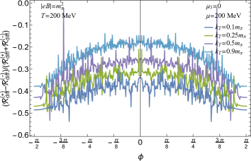
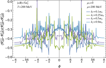
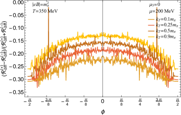
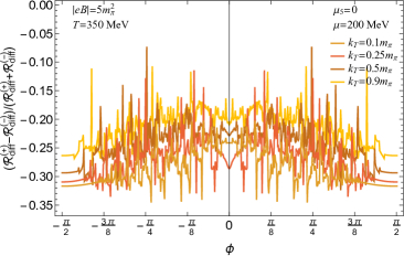
Figure 2: The degree of circular polarization as a function of the azimuthal angle for two magnetic fields, $|eB|=m_{\pi}^{2}$ (left) and $|eB|=5m_{\pi}^{2}$ (right), and two temperatures, $T=200~{}\mbox{MeV}$ (top) and $T=350~{}\mbox{MeV}$ (bottom).

The effect of a nonzero chemical potential, resulting in a predominant emission of photons with one circular polarization over the other may resemble the underlying physics of helicons (whistlers). Recall that helicons are low-frequency electromagnetic excitations in strongly magnetized plasmas, driven by the Lorentz force [26]. Their circular polarization is determined by the sign of the electric charge carriers (e.g., electrons) with higher mobility, moving in an approximately static background of opposite charges (e.g., positive ions).

For the model parameters explored, the degree of circular polarization ranges from approximately $0.12$ to $0.5$. It tends to be larger at stronger magnetic fields and lower transverse momenta (or, equivalently, lower photon energies). Comparing the top and bottom panels in Fig. 2, we also observe that the effect tends to diminish as the temperature rises.

III.2 Nonzero chiral chemical potential $\mu_{5}$

Let us now consider the case of a magnetized quark-gluon plasma (QGP) with a nonzero chiral chemical potential. Specifically, we choose $\mu_{5}=100~{}\mbox{MeV}$ as a representative value, although the actual value is not crucial for identifying the qualitative effects of $\mu_{5}$.

Fig. 3 presents sample numerical results for the emission rates of left-handed and right-handed circularly polarized photons. The data is shown for a temperature of $T=200~{}\mbox{MeV}$ and for two different magnetic field strengths: $|eB|=m_{\pi}^{2}$ (left panel) and $|eB|=5m_{\pi}^{2}$ (right panel). Although we do not show the rates at $T=350~{}\mbox{MeV}$, we have verified that they exhibit a similar qualitative behavior, albeit with generally higher values.

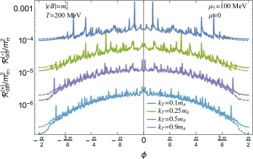
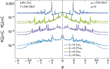
Figure 3: The angular dependence of right-handed (solid lines) and left-handed (dashed lines) circularly polarized photon emission rates for two magnetic fields, $|eB|=m_{\pi}^{2}$ (left) and $|eB|=5m_{\pi}^{2}$ (right), and fixed temperature, $T=200~{}\mbox{MeV}$.

The emission rates in Fig. 3 possess an interesting property, namely they are asymmetric with respect to reflection in the transverse plane (i.e., $\phi\to-\phi$). To visualize this effect, we construct the following two observables:

$${\cal P}^{(+)}_{\rm asym}(k_{T},\phi,y) = \frac{{\cal R}^{(+)}_{\rm diff}(k_{T},\phi,y)-{\cal R}^{(+)}_{\rm diff}(k_{T},-\phi,y)}{{\cal R}^{(+)}_{\rm diff}(k_{T},\phi,y)+{\cal R}^{(+)}_{\rm diff}(k_{T},-\phi,y)},$$ (17)

$${\cal P}^{(-)}_{\rm asym}(k_{T},\phi,y) = \frac{{\cal R}^{(-)}_{\rm diff}(k_{T},\phi,y)-{\cal R}^{(-)}_{\rm diff}(k_{T},-\phi,y)}{{\cal R}^{(-)}_{\rm diff}(k_{T},\phi,y)+{\cal R}^{(-)}_{\rm diff}(k_{T},-\phi,y)},$$ (18)

to measure the degree of emission asymmetry for the left-handed and the right-handed circularly polarized photons, respectively. It is sufficient to define them only for positive azimuthal angles in the range $0\leq\phi\leq\pi/2$. The corresponding numerical results for the emission asymmetry ${\cal P}^{(+)}_{\rm asym}(k_{T},\phi,y)$ are presented in Fig. 4 for two magnetic fields, $|eB|=m_{\pi}^{2}$ (left) and $|eB|=5m_{\pi}^{2}$ (right), and two temperatures, $T=200~{}\mbox{MeV}$ (top) and $T=350~{}\mbox{MeV}$ (bottom). We do not show any numerical data for ${\cal P}^{(-)}_{\rm asym}(k_{T},\phi,y)$ because it is not truly independent. Indeed, ${\cal P}^{(-)}_{\rm asym}(k_{T},\phi,y)=-{\cal P}^{(+)}_{\rm asym}(k_{T},\phi,y)$. As we will see later, this relation will not remain valid at nonzero $\mu$.

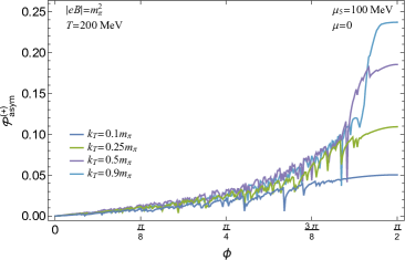
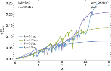
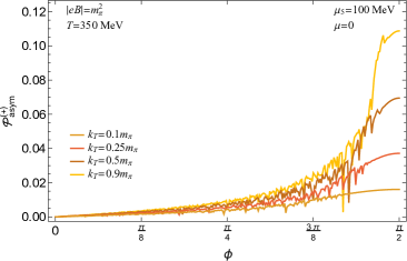
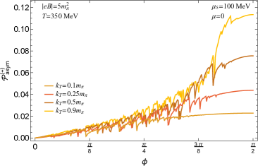
Figure 4: The emission asymmetry for the right-handed circularly polarized photons as a function of the azimuthal angular for two magnetic fields, $|eB|=m_{\pi}^{2}$ (left) and $|eB|=5m_{\pi}^{2}$ (right), and two temperatures, $T=200~{}\mbox{MeV}$ (top) and $T=350~{}\mbox{MeV}$ (bottom).

Fig 4 shows that for a positive $\mu_{5}$, the emission asymmetry is positive for photons with the right-handed circular polarization. Since ${\cal P}^{(-)}_{\rm asym}(k_{T},\phi,y)=-{\cal P}^{(+)}_{\rm asym}(k_{T},\phi,y)$, the asymmetry is negative for photons with left-handed circular polarization. This implies that the emission rate for right-handed polarized photons is higher in the direction along the magnetic field, while for left-handed polarized photons, it is higher in the direction opposite to the magnetic field. Additionally, we find that the degree of asymmetry is most pronounced at $\phi\simeq\pi/2$ and that its magnitude increases with increasing transverse momentum. We also observe that the asymmetry grows with increasing magnetic field strength but diminishes with rising temperature.

III.3 Nonzero quark-number and chiral chemical potentials $\mu$ and $\mu_{5}$

After considering the effects of $\mu$ and $\mu_{5}$ separately in the previous two subsections, let us now study their combined effect on polarized photon emission. As one might expect, the emission is characterized by a combined set of the same qualitative features, namely (i) the overall degree of circular polarization, indicating that the emission of one circular polarization dominates over the other and (ii) the degree of asymmetry for each circular polarization with respect $\phi\to-\phi$, measuring how asymmetric is the emission rate with respect to reflection in the transverse plane.

To quantify the effects in the case of nonzero $\mu$ and $\mu_{5}$, we use the same set of observables that we introduced earlier, namely ${\cal P}_{\rm circ}(k_{T},\phi,y)$ in Eq. (16), ${\cal P}^{(+)}_{\rm asym}(k_{T},\phi,y)$ in Eq. (17), and ${\cal P}^{(-)}_{\rm asym}(k_{T},\phi,y)$ in Eq. (18).

The numerical results for the overall degree of circular polarization in photon emission are presented in Fig. 5. The magnitude of the effect is comparable to that discussed in Sec. III.1, and the qualitative dependence on the strength of the magnetic field, temperature, and transverse momentum is similar. However, there is a significant difference too. The angular dependence is not symmetric under the reflection $\phi\to-\phi$. The degree of circular polarization is larger in magnitude in the direction opposite to the magnetic field. Of course, this is expected since the dominant left-handed emission is asymmetric.

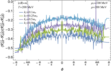
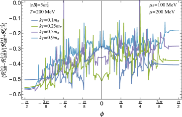
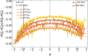
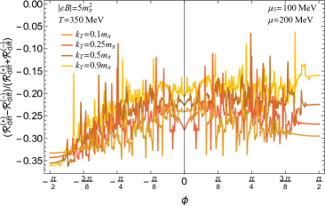
Figure 5: The degree of circular polarization as a function of the azimuthal angle for two magnetic fields, $|eB|=m_{\pi}^{2}$ (left) and $|eB|=5m_{\pi}^{2}$ (right), and two temperatures, $T=200~{}\mbox{MeV}$ (top) and $T=350~{}\mbox{MeV}$ (bottom).

The degrees of asymmetry for the emission of photons of both circular polarizations are shown in Fig. 6 for two magnetic fields, $|eB|=m_{\pi}^{2}$ (left panels) and $|eB|=5m_{\pi}^{2}$ (right panels), and two temperatures, $T=200~{}\mbox{MeV}$ (top panels) and $T=350~{}\mbox{MeV}$ (bottom panels). For both temperatures, the degree of asymmetry for the right-handed emission is larger than for the left-handed emission. The largest asymmetry is seen around $\phi\simeq\pi/2$, with the magnitudes lying in the range from about $0.12$ (right-handed) to $0.3$ (left-handed) at $T=200~{}\mbox{MeV}$ and from about $0.08$ (right-handed) to $0.13$ (left-handed) at $T=350~{}\mbox{MeV}$.

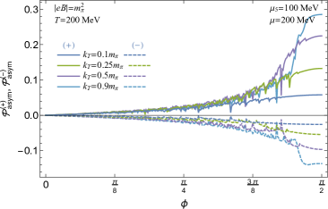
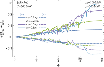
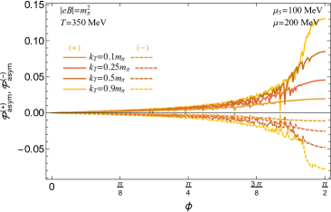
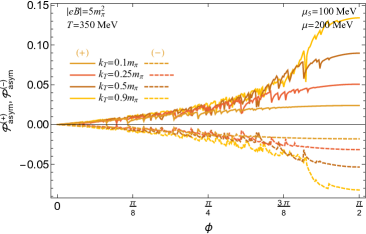
Figure 6: The emission asymmetry for the right-handed (solid lines) and left-handed (dashed lines) circularly polarized photons as a function of the azimuthal angular for two magnetic fields, $|eB|=m_{\pi}^{2}$ (left) and $|eB|=5m_{\pi}^{2}$ (right), and two temperatures, $T=200~{}\mbox{MeV}$ (top) and $T=350~{}\mbox{MeV}$ (bottom).

IV Discussion and Summary

In this study, we considered the effect of nonzero quark-number (electric charge) and chiral chemical potentials on the polarization of photon emission from a strongly magnetized QGP. In particular, we showed that the composition of circularly polarized photon emission changes in qualitative ways when the charge densities are nonzero.

A nonzero quark-number (electrical charge) density produces an overall dominance of one circular polarization over the other. For example, when the QGP has a positive quark-number (electrical charge) chemical potential ($\mu>0$), the emission rate of left-handed circular polarization photons dominates over the rate of right-handed circular polarization photons. In effect, such polarized emission can be viewed as a photon equivalent of the Hall effect in a plasma with a nonzero charge density.

It should be mention that the circularly polarized photon emission rates are symmetric with respect to the reflection in the transverse (reaction) plane when the electrical charge density is nonzero ($\mu\neq 0$), assuming the chiral charge density vanishes ($\mu_{5}=0$). However, this changes at nonzero chiral charge density ($\mu_{5}\neq 0$). When $\mu_{5}>0$, we show that the emission rate of right-handed (left-handed) circularly polarized photons is higher in the upper (lower) hemisphere. (Here the two hemispheres are defined by the magnetic field direction.) The roles of the two circular polarizations interchange when the sign of $\mu_{5}$ changes.

As expected, the combined effect of nonzero electrical and chiral charge densities in the QPG is given by a superposition of their individual effects. Generally, a nonzero electrical charge leads to an overall dominance of the photon emission with one circular polarization over the other. The additional chiral charge density produces spatial asymmetries (with respect to reflection in the transverse plane) in photon emission for each circular polarization. Moreover, while the rate for one circular polarization is higher in the upper hemisphere, the rate for the other circular polarization is higher in the lower hemisphere.

Our findings suggest that the composition of circularly polarized photon emission and its asymmetry with respect to reflection in the transverse plane can be used as unambiguous observable signatures of nonzero electrical and chiral charge densities in a strongly magnetized plasma.

Appendix A Matsubara sums

In the calculation of the polarization tensor in the main text, we perform Matsubara sums by using the following general result:

$$T\sum_{k=-\infty}^{\infty}\frac{(i\omega_{k}+\mu+s\mu_{5})(i\omega_{k}-i\Omega_{m}+\mu+s\mu_{5})X+(i\omega_{k}+\mu+s\mu_{5})Y_{1}+(i\omega_{k}-i\Omega_{m}+\mu+s\mu_{5})Y_{2}+Z}{\left[(i\omega_{k}+\mu+s\mu_{5})^{2}-a^{2}\right]\left[(i\omega_{k}-i\Omega_{m}+\mu+s\mu_{5})^{2}-b^{2}\right]}$$

$$=\sum_{\lambda=\pm 1}\sum_{\eta=\pm 1}\frac{\left[n_{F}(a+\eta\mu+\eta s\mu_{5})-n_{F}(\lambda b+\eta\mu+\eta s\mu_{5})\right]}{4\lambda ab\left(a-\lambda b+\eta i\Omega_{m}\right)}\left[\lambda abX-\eta\left(aY_{1}+\lambda bY_{2}\right)+Z\right],$$ (19)

where coefficient $X$, $Y_{1}$, $Y_{2}$, and $Z$ are arbitrary functions of momenta. In the calculation of the polarization tensor, parameters $a$ and $b$ are replaced with the Landau level energies, $E_{n,p_{z},f}=\sqrt{p_{z}^{2}+2n|e_{f}B|}$ and $E_{n^{\prime},p_{z}-k_{z},f}=\sqrt{(p_{z}-k_{z})^{2}+2n^{\prime}|e_{f}B|}$.

Note that the expression in the parenthesis of the final result in Eq. (19) can be formally obtained from the numerator of the original expression by making the following replacements: $(i\omega_{k}+s\mu_{5})(i\omega_{k}-i\Omega_{m}+s\mu_{5})\to\lambda ab$, $(i\omega_{k}+s\mu_{5})\to-\eta a$, and $(i\omega_{k}-i\Omega_{m}+s\mu_{5})\to-\eta\lambda b$.

Appendix B Dirac traces

In the derivation of the photon polarization function, one has to calculate four different types of Dirac traces. For completeness, here we present the corresponding results:

$$T_{1,f}^{\mu\nu}(s_{1},s_{2}) = \,\mbox{tr}\left\{\gamma^{\mu}\left(\bar{p}_{\parallel}\gamma_{\parallel}-\mu_{5}\gamma^{0}\gamma^{5}\right)\left(\mathcal{P}_{+}^{f}L_{n}+\mathcal{P}_{-}^{f}L_{n-1}\right)\mathcal{P}_{5}^{s_{1}}\gamma^{\nu}\left((\bar{p}_{\parallel}-k_{\parallel})\gamma_{\parallel}-\mu_{5}\gamma^{0}\gamma^{5}\right)\left(\mathcal{P}_{+}^{f}L_{n^{\prime}}+\mathcal{P}_{-}^{f}L_{n^{\prime}-1}\right)\mathcal{P}_{5}^{s_{2}}\right\},$$

$$T_{2,f}^{\mu\nu}(s_{1},s_{2}) = \frac{i}{\ell_{f}^{2}}\,\mbox{tr}\left\{\gamma^{\mu}\left(\bar{p}_{\parallel}\gamma_{\parallel}-\mu_{5}\gamma^{0}\gamma^{5}\right)\left(\mathcal{P}_{+}^{f}L_{n}+\mathcal{P}_{-}^{f}L_{n-1}\right)\mathcal{P}_{5}^{s_{1}}\gamma^{\nu}(\mathbf{r}_{\perp}\cdot\bm{\gamma}_{\perp})L_{n^{\prime}-1}^{1}\mathcal{P}_{5}^{s_{2}}\right\},$$ (21)

$$T_{3,f}^{\mu\nu}(s_{1},s_{2}) = -\frac{i}{\ell_{f}^{2}}\,\mbox{tr}\left\{\gamma^{\mu}(\mathbf{r}_{\perp}\cdot\bm{\gamma}_{\perp})L_{n-1}^{1}\mathcal{P}_{5}^{s_{1}}\gamma^{\nu}\left[(\bar{p}_{\parallel}-k_{\parallel})\gamma_{\parallel}-\mu_{5}\gamma^{0}\gamma^{5}\right]\left(\mathcal{P}_{+}^{f}L_{n^{\prime}}+\mathcal{P}_{-}^{f}L_{n^{\prime}-1}\right)\mathcal{P}_{5}^{s_{2}}\right\},$$ (22)

$$T_{4,f}^{\mu\nu}(s_{1},s_{2}) = \frac{1}{\ell_{f}^{4}}\,\mbox{tr}\left\{\gamma^{\mu}(\mathbf{r}_{\perp}\cdot\bm{\gamma}_{\perp})L_{n-1}^{1}\mathcal{P}_{5}^{s_{1}}\gamma^{\nu}(\mathbf{r}_{\perp}\cdot\bm{\gamma}_{\perp})L_{n^{\prime}-1}^{1}\mathcal{P}_{5}^{s_{2}}\right\},$$ (23)

where we introduced the shorthand notation $\bar{p}_{\parallel}\gamma_{\parallel}=\bar{p}_{0}\gamma^{0}-p^{3}\gamma^{3}$ and $\bar{p}_{0}=p_{0}+\mu$. Also, for brevity of presentation, we omitted the explicit dependence of all functions on their arguments, i.e., $L_{n}^{\alpha}\equiv L_{n}^{\alpha}\left(\zeta\right)$, where $\zeta=r_{\perp}^{2}/(2\ell_{f}^{2})$.

Appendix C Polarization projections of the traces

Here we separate the results of traces in Eqs. (B) – (23) into individual polarization contributions. By using the definition in Eq. (2), we introduce the following polarization projections:

$$\mathcal{T}_{0}^{f}(s_{1},s_{2}) = \epsilon_{0}^{\mu}\epsilon_{0}^{\nu*}\sum_{i=1}^{4}T_{i,f}^{\mu\nu}(s_{1},s_{2}),$$ (24)

$$\mathcal{T}_{-}^{f}(s_{1},s_{2}) = -\epsilon_{-}^{\mu}\epsilon_{-}^{\nu*}\sum_{i=1}^{4}T_{i,f}^{\mu\nu}(s_{1},s_{2}),$$ (25)

$$\mathcal{T}_{+}^{f}(s_{1},s_{2}) = -\epsilon_{+}^{\mu}\epsilon_{+}^{\nu*}\sum_{i=1}^{4}T_{i,f}^{\mu\nu}(s_{1},s_{2}),$$ (26)

$$\mathcal{T}_{\parallel}^{f}(s_{1},s_{2}) = \epsilon_{\parallel}^{\mu}\epsilon_{\parallel}^{\nu*}\sum_{i=1}^{4}T_{i,f}^{\mu\nu}(s_{1},s_{2}).$$ (27)

For each function, the result is nonzero only when $s_{1}=s_{2}$. The corresponding nonvanishing results read

$$\mathcal{T}_{0}^{f}(s,s) = \left[(\bar{p}_{0}-\mu_{5}-p_{z}s_{\perp}s)(\bar{p}_{0}-k_{0}-s\mu_{5})+(p_{z}-k_{z})\left(p_{z}-s_{\perp}s\bar{p}_{0}+s_{\perp}\mu_{5}\right)\right]L_{n}L_{n^{\prime}}$$ (28)

$$+ \left[(\bar{p}_{0}-s\mu_{5}+p_{z}s_{\perp}s)(\bar{p}_{0}-k_{0}-s\mu_{5})+(p_{z}-k_{z})(p_{z}+s_{\perp}s\bar{p}_{0}-s_{\perp}s\mu_{5})\right]L_{n-1}L_{n^{\prime}-1}$$

$$+ \frac{2r_{\perp}^{2}}{\ell_{f}^{4}}L_{n-1}^{1}L_{n^{\prime}-1}^{1},$$

$$\mathcal{T}_{-}^{f}(s,s) = (s\bar{p}_{0}+p_{z}-\mu_{5})(sk_{0}-s\bar{p}_{0}-k_{z}+p_{z}+\mu_{5})\left[L_{n-1}L_{n^{\prime}}(1+s_{\perp})+L_{n}L_{n^{\prime}-1}(1-s_{\perp})\right],$$ (29)

$$\mathcal{T}_{+}^{f}(s,s) = (s\bar{p}_{0}-p_{z}-\mu_{5})(sk_{0}-s\bar{p}_{0}+k_{z}-p_{z}+\mu_{5})\left[L_{n}L_{n^{\prime}-1}(1+s_{\perp})+L_{n-1}L_{n^{\prime}}(1-s_{\perp})\right],$$ (30)

$$\mathcal{T}_{\parallel}^{f}(s,s) = -\mathcal{T}_{0}^{f}(s,s)+\frac{4L_{n-1}^{1}L_{n^{\prime}-1}^{1}r_{\perp}^{2}}{\ell_{f}^{4}}.$$ (31)

Appendix D Integration over $r_{\perp}$

We have the following results for the integrals:

$$\mathcal{J}^{f}_{0}(s,s) = \int d^{2}\mathbf{r}_{\perp}e^{-i\mathbf{r}_{\perp}\cdot\mathbf{k}_{\perp}}e^{-\mathbf{r}_{\perp}^{2}/(2\ell_{f}^{2})}\mathcal{T}_{0}^{f}(s,s)$$ (32)

$$= 2\pi\ell_{f}^{2}\left[(\bar{p}_{0}-\mu_{5}-p_{z}s_{\perp}s)(\bar{p}_{0}-k_{0}-s\mu_{5})+(p_{z}-k_{z})\left(p_{z}-s_{\perp}s\bar{p}_{0}+s_{\perp}\mu_{5}\right)\right]\,\mathcal{I}_{0,f}^{n,n^{\prime}}$$

$$+ 2\pi\ell_{f}^{2}\left[(\bar{p}_{0}-s\mu_{5}+p_{z}s_{\perp}s)(\bar{p}_{0}-k_{0}-s\mu_{5})+(p_{z}-k_{z})(p_{z}+s_{\perp}s\bar{p}_{0}-s_{\perp}s\mu_{5})\right]\,\mathcal{I}_{0,f}^{n-1,n^{\prime}-1}(\xi)$$

$$+ 8\pi\,\mathcal{I}_{2,f}^{n-1,n^{\prime}-1}(\xi),$$

$$\mathcal{J}^{f}_{-}(s,s) = \int d^{2}\mathbf{r}_{\perp}e^{-i\mathbf{r}_{\perp}\cdot\mathbf{k}_{\perp}}e^{-\mathbf{r}_{\perp}^{2}/(2\ell_{f}^{2})}\mathcal{T}_{+}^{f}(s,s)$$ (33)

$$= 2\pi\ell_{f}^{2}(s\bar{p}_{0}+p_{z}-\mu_{5})(sk_{0}-s\bar{p}_{0}-k_{z}+p_{z}+\mu_{5})\left[(1+s_{\perp})\mathcal{I}_{0,f}^{n-1,n^{\prime}}(\xi)+(1-s_{\perp})\mathcal{I}_{0,f}^{n,n^{\prime}-1}(\xi)\right],$$

$$\mathcal{J}^{f}_{+}(s,s) = \int d^{2}\mathbf{r}_{\perp}e^{-i\mathbf{r}_{\perp}\cdot\mathbf{k}_{\perp}}e^{-\mathbf{r}_{\perp}^{2}/(2\ell_{f}^{2})}\mathcal{T}_{-}^{f}(s,s)$$ (34)

$$= 2\pi\ell_{f}^{2}(s\bar{p}_{0}-p_{z}-\mu_{5})(sk_{0}-s\bar{p}_{0}+k_{z}-p_{z}+\mu_{5})\left[(1+s_{\perp})\mathcal{I}_{0,f}^{n,n^{\prime}-1}(\xi)+(1-s_{\perp})\mathcal{I}_{0,f}^{n-1,n^{\prime}}(\xi)\right],$$

$$\mathcal{J}^{f}_{\parallel}(s,s) = \int d^{2}\mathbf{r}_{\perp}e^{-i\mathbf{r}_{\perp}\cdot\mathbf{k}_{\perp}}e^{-\mathbf{r}_{\perp}^{2}/(2\ell_{f}^{2})}\mathcal{T}_{\parallel}^{f}(s,s)=8\pi\,\mathcal{I}_{2,f}^{n-1,n^{\prime}-1}(\xi)-\mathcal{J}^{f}_{0}(s,s).$$ (35)

where $\xi=k_{\perp}^{2}\ell_{f}^{2}/2$ and functions

$$\mathcal{I}_{0,f}^{n,n^{\prime}}(\xi) = \frac{(n^{\prime})!}{n!}e^{-\xi}\xi^{n-n^{\prime}}\left(L_{n^{\prime}}^{n-n^{\prime}}\left(\xi\right)\right)^{2}=\frac{n!}{(n^{\prime})!}e^{-\xi}\xi^{n^{\prime}-n}\left(L_{n}^{n^{\prime}-n}\left(\xi\right)\right)^{2},$$ (36)

$$\mathcal{I}_{2,f}^{n,n^{\prime}}(\xi) = \frac{n+n^{\prime}+2}{2}\left[\mathcal{I}_{0,f}^{n,n^{\prime}}(\xi)+\mathcal{I}_{0,f}^{n+1,n^{\prime}+1}(\xi)\right]-\frac{\xi}{2}\left[\mathcal{I}_{0,f}^{n+1,n^{\prime}}(\xi)+\mathcal{I}_{0,f}^{n,n^{\prime}+1}(\xi)\right]$$ (37)

are the same as those introduced in Ref. [22].

Appendix E Polarization projections of the imaginary part of $\Pi^{\mu\nu}(\Omega;\mathbf{k})$

The polarization projections of the imaginary part of $\Pi^{\mu\nu}(i\Omega_{m};\mathbf{k})$ are given by the following formal expressions:

$$\Pi^{(i)}(i\Omega_{m};\mathbf{k})=-\sum_{f=u,d}\frac{N_{c}\alpha_{f}T}{\pi\ell_{f}^{4}}\sum_{n,n^{\prime}=0}^{\infty}\sum_{k=-\infty}^{\infty}\sum_{s=\pm 1}\int\frac{dp_{z}}{2\pi}\frac{\mathcal{J}_{(i)}^{f}(-s,-s)}{[(i\omega_{k}+\mu+s\mu_{5})^{2}-E_{n,p_{z},f}^{2}][(i\omega_{k}+\mu-i\Omega_{m}+s\mu_{5})^{2}-E_{n^{\prime},p_{z}-k_{z},f}^{2}]}.$$ (38)

By using Matsubara sum in Appendix A, we derive

$$\Pi^{(i)}(i\Omega_{m};\mathbf{k})=-\sum_{f=u,d}\frac{N_{c}\alpha_{f}}{\pi\ell_{f}^{4}}\sum_{n,n^{\prime}=0}^{\infty}\sum_{s,\eta,\lambda=\pm 1}\int\frac{dp_{z}}{2\pi}\frac{[n_{F}(E_{n,p_{z},f}+\eta\mu+\eta s\mu_{5})-n_{F}(\lambda E_{n^{\prime},p_{z}-k_{z},f}+\eta\mu+\eta s\mu_{5})]\mathcal{F}^{(i)}_{s,f}(\xi,i\Omega_{m})}{4\lambda E_{n,p_{z},f}E_{n^{\prime},p_{z}-k_{z},f}\left[E_{n,p_{z},f}-\lambda E_{n^{\prime},p_{z}-k_{z},f}+i\eta\Omega_{m}\right]},$$ (39)

where

$$\mathcal{F}^{(0)}_{s,f}(\xi,i\Omega_{m}) = 2\pi\ell_{f}^{2}\left(p_{z}-s_{\perp}s\eta E_{n,p_{z},f}\right)\left[p_{z}-k_{z}-s_{\perp}s\eta\lambda E_{n^{\prime},p_{z}-k_{z},f}\right]\mathcal{I}_{0,f}^{n,n^{\prime}}(\xi)$$ (40)

$$+ 2\pi\ell_{f}^{2}\left(p_{z}+s_{\perp}s\eta E_{n,p_{z},f}\right)\left[p_{z}-k_{z}+s_{\perp}s\eta\lambda E_{n^{\prime},p_{z}-k_{z},f}\right]\mathcal{I}_{0,f}^{n-1,n^{\prime}-1}(\xi)+4\pi\mathcal{I}_{2,f}^{n-1,n^{\prime}-1}(\xi),$$

$$\mathcal{F}^{(-)}_{s,f}(\xi,i\Omega_{m}) = 2\pi\ell_{f}^{2}\left[p_{z}(p_{z}-k_{z})-k_{z}s\eta E_{n,p_{z},f}-p_{z}si\Omega_{m}-\lambda E_{n,p_{z},f}E_{n^{\prime},p_{z}-k_{z},f}\right]$$ (41)

$$\times \left[(1+s_{\perp})\mathcal{I}_{0,f}^{n-1,n^{\prime}}(\xi)+(1-s_{\perp})\mathcal{I}_{0,f}^{n,n^{\prime}-1}(\xi)\right],$$

$$\mathcal{F}^{(+)}_{s,f}(\xi,i\Omega_{m}) = 2\pi\ell_{f}^{2}\left[p_{z}(p_{z}-k_{z})+k_{z}s\eta E_{n,p_{z},f}+p_{z}si\Omega_{m}-\lambda E_{n,p_{z},f}E_{n^{\prime},p_{z}-k_{z},f}\right]$$ (42)

$$\times \left[(1+s_{\perp})\mathcal{I}_{0,f}^{n,n^{\prime}-1}(\xi)+(1-s_{\perp})\mathcal{I}_{0,f}^{n-1,n^{\prime}}(\xi)\right],$$

$$\mathcal{F}^{(\parallel)}_{s,f}(\xi,i\Omega_{m}) = -\mathcal{F}^{(0)}_{s,f}(\xi,i\Omega_{m})+8\pi\mathcal{I}_{2,f}^{n-1,n^{\prime}-1}(\xi).$$ (43)

After replacing $i\Omega_{m}\to\Omega+i\epsilon$ and using the Sokhotski formula, we extract the following imaginary part of the polarization functions:

$$\mbox{Im}\Pi^{(i)}(\Omega;\mathbf{k}) = \sum_{f=u,d}\frac{N_{c}\alpha_{f}}{\ell_{f}^{4}}\sum_{n,n^{\prime}=0}^{\infty}\sum_{s,\eta,\lambda=\pm 1}\int\frac{dp_{z}}{2\pi}\frac{[n_{F}(E_{n,p_{z},f}+\eta\mu+\eta s\mu_{5})-n_{F}(\lambda E_{n^{\prime},p_{z}-k_{z},f}+\eta\mu+\eta s\mu_{5})]}{4\lambda E_{n,p_{z},f}E_{n^{\prime},p_{z}-k_{z},f}}$$ (44)

$$\times \mathcal{F}_{s,f}^{(i)}(\xi,\Omega)\,\delta\left(E_{n,p_{z},f}-\lambda E_{n^{\prime},p_{z}-k_{z},f}+\eta\Omega\right).$$

The solutions of the energy conservation equation $E_{n,p_{z},f}-\lambda E_{n^{\prime},p_{z}-k_{z},f}+\eta\Omega=0$ are given by the following explicit expressions [21, 22, 27]:

$$p_{z,f}^{(\pm)} = \frac{k_{z}}{2}\left[1+\frac{2(n-n^{\prime})|e_{f}B|}{\Omega^{2}-k_{z}^{2}}\pm\frac{\Omega}{|k_{z}|}\sqrt{\left(1-\frac{(k_{-}^{f})^{2}}{\Omega^{2}-k_{z}^{2}}\right)\left(1-\frac{(k_{+}^{f})^{2}}{\Omega^{2}-k_{z}^{2}}\right)}\right].$$ (45)

The corresponding fermions energies, satisfying the energy conservation relation, are

$$\left.E_{n,p_{z},f}\right|_{p_{z}=p_{z,f}^{(\pm)}}=-\frac{\eta\Omega}{2}\left[1+\frac{2(n-n^{\prime})|e_{f}B|}{\Omega^{2}-k_{z}^{2}}\pm\frac{|k_{z}|}{\Omega}\sqrt{\left(1-\frac{(k_{-}^{f})^{2}}{\Omega^{2}-k_{z}^{2}}\right)\left(1-\frac{(k_{+}^{f})^{2}}{\Omega^{2}-k_{z}^{2}}\right)}\right],$$ (46a)

$$\left.E_{n^{\prime},p_{z}-k_{z},f}\right|_{p_{z}=p_{z,f}^{(\pm)}}=\frac{\lambda\eta\Omega}{2}\left[1-\frac{2(n-n^{\prime})|e_{f}B|}{\Omega^{2}-k_{z}^{2}}\mp\frac{|k_{z}|}{\Omega}\sqrt{\left(1-\frac{(k_{-}^{f})^{2}}{\Omega^{2}-k_{z}^{2}}\right)\left(1-\frac{(k_{+}^{f})^{2}}{\Omega^{2}-k_{z}^{2}}\right)}\right].$$ (46b)

By making use of these solutions, we can easily perform the integration over the longitudinal momentum $p_{z}$ in Eq. (44). The result reads

$$\mbox{Im}\Pi^{(i)}(\Omega;\mathbf{k}) = \sum_{f=u,d}\frac{N_{c}\alpha_{f}}{4\pi\ell_{f}^{4}}\sum_{n,n^{\prime}=0}^{\infty}\sum_{s,s^{\prime},\eta,\lambda=\pm 1}\Theta_{\lambda,\eta}^{n,n^{\prime}}(\Omega,k_{z})\mathcal{F}_{s,f}^{(i)}(\xi,\Omega)$$ (47)

$$\times \frac{n_{F}(E_{n,p_{z},f}+\eta\mu+\eta s\mu_{5})-n_{F}(\lambda E_{n^{\prime},p_{z}-k_{z},f}+\eta\mu+\eta s\mu_{5})}{\eta\lambda\sqrt{\left(\Omega^{2}-k_{z}^{2}-(k_{-}^{f})^{2}\right)\left(\Omega^{2}-k_{z}^{2}-(k_{+}^{f})^{2}\right)}}\Bigg{|}_{p_{z}=p_{z,f}^{(s^{\prime})}},$$

where the threshold function $\Theta_{\lambda,\eta}^{n,n^{\prime}}(\Omega,k_{z})$ is defined as follows:

$$\Theta_{\lambda,\eta}^{n,n^{\prime}}(\Omega,k_{z})=\left\{\begin{array}[]{lll}\theta\left((k_{-}^{f})^{2}+k_{z}^{2}-\Omega^{2}\right)&\mbox{for}&\lambda=1,\eta=-1,n>n^{\prime},\\ \theta\left((k_{-}^{f})^{2}+k_{z}^{2}-\Omega^{2}\right)&\mbox{for}&\lambda=1,\eta=1,n<n^{\prime},\\ \theta\left(\Omega^{2}-k_{z}^{2}-(k_{+}^{f})^{2}\right)&\mbox{for}&\lambda=-1,\eta=-1,\end{array}\right.$$ (48)

and $\Theta_{\lambda,\eta}^{n,n^{\prime}}(\Omega,k_{z})=0$ otherwise. By definition, $\theta(x)$ is the Heaviside step function.

The explicit expressions for functions in Eqs. (40) – (43) on the solutions to the energy-momentum relation read

$$\left.\mathcal{F}_{s,f}^{(0)}(\xi,\Omega)\right|_{p_{z}=p_{z,f}^{(s^{\prime})}} = \mathcal{A}_{s,s^{\prime},f}(\xi,\Omega)+\mathcal{B}_{f}(\xi,\Omega),$$ (49)

$$\left.\mathcal{F}_{s,f}^{(-)}(\xi,\Omega)\right|_{p_{z}=p_{z,f}^{(s^{\prime})}} = \pi\ell_{f}^{2}\left(\Omega^{2}-k_{z}^{2}\right)\left[1-\frac{2(n+n^{\prime})}{\left(\Omega^{2}-k_{z}^{2}\right)\ell_{f}^{2}}-ss^{\prime}\frac{k_{z}}{|k_{z}|}\sqrt{\left(1-\frac{(k_{-}^{f})^{2}}{\Omega^{2}-k_{z}^{2}}\right)\left(1-\frac{(k_{+}^{f})^{2}}{\Omega^{2}-k_{z}^{2}}\right)}\right]$$ (50)

$$\times\left[(1+s_{\perp})\mathcal{I}_{0,f}^{n-1,n^{\prime}}(\xi)+(1-s_{\perp})\mathcal{I}_{0,f}^{n,n^{\prime}-1}(\xi)\right],$$

$$\left.\mathcal{F}_{s,f}^{(+)}(\xi,\Omega)\right|_{p_{z}=p_{z,f}^{(s^{\prime})}} = \pi\ell_{f}^{2}\left(\Omega^{2}-k_{z}^{2}\right)\left[1-\frac{2(n+n^{\prime})}{\left(\Omega^{2}-k_{z}^{2}\right)\ell_{f}^{2}}+ss^{\prime}\frac{k_{z}}{|k_{z}|}\sqrt{\left(1-\frac{(k_{-}^{f})^{2}}{\Omega^{2}-k_{z}^{2}}\right)\left(1-\frac{(k_{+}^{f})^{2}}{\Omega^{2}-k_{z}^{2}}\right)}\right]$$ (51)

$$\times\left[(1-s_{\perp})\mathcal{I}_{0,f}^{n,n^{\prime}-1}(\xi)+(1-s_{\perp})\mathcal{I}_{0,f}^{n-1,n^{\prime}}(\xi)\right],$$

$$\left.\mathcal{F}_{s,f}^{(\parallel)}(\xi,\Omega)\right|_{p_{z}=p_{z,f}^{(s^{\prime})}} = -\mathcal{A}_{s,s^{\prime},f}(\xi,\Omega)+\mathcal{B}_{f}(\xi,\Omega).$$ (52)

Here, we used the following two auxiliary functions:

$$\mathcal{A}_{s,s^{\prime},f}(\xi,\Omega) = 2\pi\frac{\Omega^{2}+k_{z}^{2}}{\Omega^{2}-k_{z}^{2}}\Bigg{\{}\frac{2(n-n^{\prime})^{2}}{\left(\Omega^{2}-k_{z}^{2}\right)\ell_{f}^{2}}-(n+n^{\prime})+\frac{2s^{\prime}\Omega|k_{z}|(n-n^{\prime})}{\Omega^{2}+k_{z}^{2}}$$ (53)

$$\times \sqrt{\left(1-\frac{(k_{-}^{f})^{2}}{\Omega^{2}-k_{z}^{2}}\right)\left(1-\frac{(k_{+}^{f})^{2}}{\Omega^{2}-k_{z}^{2}}\right)}\Bigg{\}}\left[\mathcal{I}_{0,f}^{n,n^{\prime}}(\xi)+\mathcal{I}_{0,f}^{n-1,n^{\prime}-1}(\xi)\right]$$

$$+ \frac{4\pi s_{\perp}s\Omega k_{z}}{\Omega^{2}-k_{z}^{2}}\Bigg{\{}\frac{2(n-n^{\prime})^{2}}{\left(\Omega^{2}-k_{z}^{2}\right)\ell_{f}^{2}}-(n+n^{\prime})+\frac{s^{\prime}(n-n^{\prime})(\Omega^{2}+k_{z}^{2})}{2\Omega|k_{z}|}$$

$$\times \sqrt{\left(1-\frac{(k_{-}^{f})^{2}}{\Omega^{2}-k_{z}^{2}}\right)\left(1-\frac{(k_{+}^{f})^{2}}{\Omega^{2}-k_{z}^{2}}\right)}\Bigg{\}}\left[\mathcal{I}_{0,f}^{n,n^{\prime}}(\xi)-\mathcal{I}_{0,f}^{n-1,n^{\prime}-1}(\xi)\right],$$

$$\mathcal{B}_{f}(\xi,\Omega) = 4\pi\left\{(n+n^{\prime})\left[\mathcal{I}_{0,f}^{n-1,n^{\prime}-1}(\xi)+\mathcal{I}_{0,f}^{n,n^{\prime}}(\xi)\right]-\xi\left[\mathcal{I}_{0,f}^{n,n^{\prime}-1}(\xi)+\mathcal{I}_{0,f}^{n-1,n^{\prime}}(\xi)\right]\right\}.$$ (54)

Note that $\mathcal{B}_{f}(\xi,\Omega)$ is independent of $s$ and $s^{\prime}$.

References

- Skokov et al. [2009] V. Skokov, A. Y. Illarionov, and V. Toneev, Estimate of the magnetic field strength in heavy-ion collisions, Int. J. Mod. Phys. A24, 5925 (2009), arXiv:0907.1396 .
- Voronyuk et al. [2011] V. Voronyuk, V. Toneev, W. Cassing, E. Bratkovskaya, V. Konchakovski, et al., (Electro-)magnetic field evolution in relativistic heavy-ion collisions, Phys. Rev. C 83, 054911 (2011), arXiv:1103.4239 .
- Deng and Huang [2012] W.-T. Deng and X.-G. Huang, Event-by-event generation of electromagnetic fields in heavy-ion collisions, Phys. Rev. C 85, 044907 (2012), arXiv:1201.5108 .
- Bloczynski et al. [2013] J. Bloczynski, X.-G. Huang, X. Zhang, and J. Liao, Azimuthally fluctuating magnetic field and its impacts on observables in heavy-ion collisions, Phys. Lett. B718, 1529 (2013), arXiv:1209.6594 .
- Guo et al. [2020] X. Guo, J. Liao, and E. Wang, Spin Hydrodynamic Generation in the Charged Subatomic Swirl, Sci. Rep. 10, 2196 (2020), arXiv:1904.04704 [hep-ph] .
- Jiang et al. [2016] Y. Jiang, Z.-W. Lin, and J. Liao, Rotating quark-gluon plasma in relativistic heavy ion collisions, Phys. Rev. C 94, 044910 (2016), [Erratum: Phys.Rev.C 95, 049904 (2017)], arXiv:1602.06580 [hep-ph] .
- Deng and Huang [2016] W.-T. Deng and X.-G. Huang, Vorticity in Heavy-Ion Collisions, Phys. Rev. C 93, 064907 (2016), arXiv:1603.06117 [nucl-th] .
- Sirunyan et al. [2018] A. M. Sirunyan et al. (CMS), Constraints on the chiral magnetic effect using charge-dependent azimuthal correlations in and PbPb collisions at the CERN Large Hadron Collider, Phys. Rev. C 97, 044912 (2018), arXiv:1708.01602 [nucl-ex] .
- Acharya et al. [2020] S. Acharya et al. (ALICE), Constraining the Chiral Magnetic Effect with charge-dependent azimuthal correlations in Pb-Pb collisions at = 2.76 and 5.02 TeV, J. High Energy Phys. 09, 160, arXiv:2005.14640 [nucl-ex] .
- Abdallah et al. [2022] M. S. Abdallah et al. (STAR), Search for the Chiral Magnetic Effect via Charge-Dependent Azimuthal Correlations Relative to Spectator and Participant Planes in Au+Au Collisions at = 200 GeV, Phys. Rev. Lett. 128, 092301 (2022), arXiv:2106.09243 [nucl-ex] .
- Aboona et al. [2023] B. Aboona et al. (STAR), Search for the Chiral Magnetic Effect in Au+Au collisions at GeV with the STAR forward Event Plane Detectors, Phys. Lett. B 839, 137779 (2023), arXiv:2209.03467 [nucl-ex] .
- Tuchin [2013] K. Tuchin, Particle production in strong electromagnetic fields in relativistic heavy-ion collisions, Adv. High Energy Phys. 2013, 490495 (2013), arXiv:1301.0099 [hep-ph] .
- Kharzeev et al. [2016] D. E. Kharzeev, J. Liao, S. A. Voloshin, and G. Wang, Chiral magnetic and vortical effects in high-energy nuclear collisions—A status report, Prog. Part. Nucl. Phys. 88, 1 (2016), arXiv:1511.04050 .
- Huang [2016] X.-G. Huang, Electromagnetic fields and anomalous transports in heavy-ion collisions — A pedagogical review, Rept. Prog. Phys. 79, 076302 (2016), arXiv:1509.04073 .
- Miransky and Shovkovy [2015] V. A. Miransky and I. A. Shovkovy, Quantum field theory in a magnetic field: From quantum chromodynamics to graphene and Dirac semimetals, Phys. Rept. 576, 1 (2015), arXiv:1503.00732 .
- Kharzeev et al. [2024] D. E. Kharzeev, J. Liao, and P. Tribedy, Chiral Magnetic Effect in Heavy Ion Collisions: The Present and Future, (2024), arXiv:2405.05427 [nucl-th] .
- Abdulhamid et al. [2023] M. I. Abdulhamid et al. (STAR), Event-by-event correlations between (¯) hyperon global polarization and handedness with charged hadron azimuthal separation in Au+Au collisions at GeV from STAR, Phys. Rev. C 108, 014909 (2023), arXiv:2304.10037 [nucl-ex] .
- Yee [2013] H.-U. Yee, Flows and polarization of early photons with magnetic field at strong coupling, Phys. Rev. D 88, 026001 (2013), arXiv:1303.3571 [nucl-th] .
- Mamo and Yee [2013] K. A. Mamo and H.-U. Yee, Spin polarized photons and dileptons from axially charged plasma, Phys. Rev. D 88, 114029 (2013), arXiv:1307.8099 [nucl-th] .
- Mamo and Yee [2016] K. A. Mamo and H.-U. Yee, Spin polarized photons from an axially charged plasma at weak coupling: Complete leading order, Phys. Rev. D 93, 065053 (2016), arXiv:1512.01316 [hep-ph] .
- Wang et al. [2020] X. Wang, I. A. Shovkovy, L. Yu, and M. Huang, Ellipticity of photon emission from strongly magnetized hot QCD plasma, Phys. Rev. D 102, 076010 (2020), arXiv:2006.16254 .
- Wang and Shovkovy [2021a] X. Wang and I. Shovkovy, Photon polarization tensor in a magnetized plasma: Absorptive part, Phys. Rev. D 104, 056017 (2021a), arXiv:2103.01967 [nucl-th] .
- Kapusta and Gale [2011] J. I. Kapusta and C. Gale, Finite-Temperature Field Theory: Principles and Applications, Cambridge Monographs on Mathematical Physics (Cambridge University Press, 2011).
- Hattori et al. [2021] K. Hattori, H. Taya, and S. Yoshida, Di-lepton production from a single photon in strong magnetic fields: vacuum dichroism, J. High Energy Phys. 01, 093, arXiv:2010.13492 [hep-ph] .
- Gradshteyn and Ryzhik [1980] I. S. Gradshteyn and I. M. Ryzhik, Table of integrals, series and products (Academic Press, Orlando, 1980).
- Maxfield [1969] B. W. Maxfield, Helicon waves in solids, Am. J. Phys. 37, 241 (1969).
- Wang and Shovkovy [2021b] X. Wang and I. Shovkovy, Polarization tensor of magnetized quark-gluon plasma at nonzero baryon density, Eur. Phys. J. C 81, 901 (2021b), arXiv:2106.09029 [nucl-th] .