Thermal False Vacuum Decay Is Not What It Seems

Abstract

We study the decay of a thermally excited metastable vacuum in classical field theory using real-time numerical simulations. We find a lower decay rate than predicted by standard thermal theory. The discrepancy is due to the violation of thermal equilibrium during the critical bubble nucleation. It is reduced by introducing dissipation and noise. We propose a criterion for the system to remain in equilibrium during the nucleation process and show that it is violated in the Hamiltonian evolution of a single field. In the case of many fields, the fulfillment of the criterion is model-dependent.

Introduction — The decay of a metastable state (false vacuum) plays an important role in many branches of physics. It corresponds to first-order phase transitions in condensed matter systems and relativistic field theories Onuki (2002); Quiros (1999). In cosmology, such phase transitions have been extensively studied in the context of baryon asymmetry generation Bodeker and Buchmuller (2021) and as possible sources of gravity waves Caprini and Figueroa (2018); Caprini et al. (2020). The current electroweak vacuum of the Standard Model may be metastable Buttazzo et al. (2013); Bednyakov et al. (2015), implying its decay in the future. There are several proposals to realize false vacuum decay using cold atom systems Fialko et al. (2015, 2017); Braden et al. (2018); Billam et al. (2019); Braden et al. (2019a); Billam et al. (2022); Jenkins et al. (2024, 2023), and the first successful experiment was reported in Zenesini et al. (2024).

In many physical situations, the initial state of the system is an equilibrium thermal state around the false vacuum with some temperature $T$. The traditional approach to this case is based on the Euclidean path integral method Kobzarev et al. (1974); Coleman (1977); Callan and Coleman (1977); Linde (1981, 1983), which relates the decay rate to the imaginary part of the metastable vacuum free energy. At high enough temperatures, the transition proceeds via formation of a critical bubble – an unstable solution of the classical field equations that can decay both to the false and the true vacuum. It corresponds to the saddle point of the potential barrier separating the two vacua. The Euclidean approach then yields the decay rate in the form Affleck (1981),

$$\Gamma=\frac{\omega_{-}}{\pi T}\cdot\frac{\text{Im}F}{\cal V}\,,$$ (1)

where $\omega_{-}$ is the growth rate of the critical bubble’s unstable mode and ${\cal V}$ is the volume of the system. The imaginary part of the free energy in the false vacuum contains the Boltzmann suppression by the critical bubble energy, $\text{Im}F\propto\text{e}^{-E_{b}/T}$, as well as the determinant of the operator describing small fluctuations around it Weinberg (2012).

At $\omega_{-}\ll T\ll E_{b}$, the result (1) can also be obtained by purely classical methods. Langer Langer (1969) considered a classical multi-dimensional statistical system with dissipation and noise provided by an external heat bath and controlled by the friction parameter $\eta$. False vacuum decay then occurs as a result of diffusion in phase space, and the solution of the corresponding Fokker-Planck equation yields the rate Hanggi et al. (1990),

$$\Gamma=\frac{1}{\pi T}\left(\sqrt{\omega_{-}^{2}+\frac{\eta^{2}}{4}}-\frac{\eta}{2}\right)\cdot\frac{\text{Im}F}{\cal V}\,,$$ (2)

which reduces to (1) in the limit $\eta\to 0$.

The Euclidean approach can tell us little about the dynamics of bubble nucleation. Instead, this can be captured by real-time numerical simulations Grigoriev and Rubakov (1988); Grigoriev et al. (1989a, b); Ambjorn et al. (1990); Valls and Mazenko (1990); Alford et al. (1992, 1993); Alford and Gleiser (1993); Borsanyi et al. (2000); Braden et al. (2019b); Batini et al. (2024). These have revealed rich phenomena, including oscillon precursors and non-zero bubble velocities Aguirre et al. (2012); Gleiser et al. (1991); Gleiser and Howell (2005); Gleiser et al. (2008); Pîrvu et al. (2023). In this work, we continue the real-time study of thermal false vacuum decay, focusing on the precise determination of its rate. Surprisingly, we find deviations from Eqs. (1), (2), which signal a breakdown of thermal equilibrium during bubble nucleation. We formulate the necessary condition for the validity of the standard rate calculation and show that it is generally violated in commonly studied field theories.

Setup — We consider a real scalar field in $(1+1)$ dimensions with the action

$$S=\int\!\mathrm{d}t\,\mathrm{d}x\left(-\frac{(\partial_{\mu}\phi)^{2}}{2}-\frac{m^{2}\phi^{2}}{2}+\frac{\lambda\phi^{4}}{4}\right)\,,$$ (3)

where $\lambda>0$. The false vacuum is located at $\phi=0$, and the true vacuum corresponds to the run-away ${\phi\to\pm\infty}$. The choice of the quartic potential is convenient since it allows us to determine all quantities entering the Euclidean prediction for the rate analytically. However, we have verified that none of our conclusions rely on this choice.

In the theory (3), the critical bubble profile, its energy and the growth rate of its unstable mode are:

$$\phi_{b}(x)=\sqrt{\frac{2}{\lambda}}\cdot\frac{m}{\mathop{\rm ch}\nolimits{mx}}\,,\quad E_{b}=\frac{4m^{3}}{3\lambda}\,,\quad\omega_{-}=\sqrt{3}\,m\,.$$ (4)

Evaluating the critical bubble contribution to the free energy (see Appendix A) and substituting it into the Euclidean formula (1), one obtains the nucleation rate:

$$\Gamma_{E}=\frac{6m^{2}}{\pi}\sqrt{\frac{E_{b}}{2\pi T}}\,\text{e}^{-E_{b}/T}\,.$$ (5)

Below, we compare this expression with the results of real-time numerical simulations.

Survival probability under Hamiltonian evolution — We discretize the action (3) on a periodic spatial lattice with step $a$ and length $L$ using the second-order finite-difference approximation for spatial derivatives. This leads to multi-dimensional Hamiltonian dynamics, whose classical equations are evolved using the $4^{\rm th}$-order operator-splitting pseudo-spectral method Pîrvu et al. (2024). Most runs are performed with $a\simeq 0.012/m$, $L=100/m$, and time step $\Delta t\simeq 0.8a$. We have verified the convergence of our results by varying the lattice parameters in the ranges $ma\in[5\cdot 10^{-3},4\cdot 10^{-2}]$, $mL\in[50,400]$, $\Delta t/a\in[0.4,0.8]$. The simulations were also cross-checked with an independent code Pîrvu et al. (2023) based on a $10^{\rm th}$-order Gauss-Legendre pseudo-spectral scheme, and choosing $ma=0.04$, $mL\in[80,100]$ and $\Delta t\simeq 0.17a$.

The initial conditions are picked up from an ensemble of Gaussian perturbations around the false vacuum with the thermal Rayleigh-Jeans spectrum. Namely, we decompose the field and its canonical momentum $\pi\equiv\dot{\phi}$ at $t=0$ in Fourier modes,

$$\phi_{i}=\frac{1}{\sqrt{L}}\sum_{j=0}^{N-1}\text{e}^{ik_{j}x_{i}}\tilde{\phi}_{j}\,,\quad N\equiv\frac{L}{a}\,,\quad k_{j}\equiv\frac{2\pi j}{L}\,,$$ (6)

with $\tilde{\phi}_{j}^{*}=\tilde{\phi}_{N-j}$, and similarly for $\pi_{i}$. The complex amplitudes $\tilde{\phi}_{j}$, $\tilde{\pi}_{j}$ are then drawn from independent Gaussian distributions with the variances

$$\langle|\tilde{\phi}_{j}|^{2}\rangle=T/\Omega_{j}^{2}\;,\quad\langle|\tilde{\pi}_{j}|^{2}\rangle=T\;.$$ (7)

We include the thermal correction to the mass Boyanovsky et al. (2004) in the lattice mode frequencies,

$$\Omega_{j}^{2}=\frac{2}{a^{2}}(1-\cos{ak_{j}})+m_{th}^{2}\;,\quad m_{th}^{2}=m^{2}-\frac{3\lambda T}{2m}\;.$$ (8)

For the temperatures considered in our work this correction is $\sim 15\%$ and cannot be neglected.

We generate an ensemble of simulations with temperature $T$ and monitor them until they decay into the true vacuum. At each moment of simulation time $t$, we count the number of configurations that have not yet decayed. The survival probability $P_{surv}(t)$ is then defined as the ratio of this number to the total initial number of configurations in the ensemble. This measurement is repeated for several choices of temperature in the range $0.09\leqslant\lambda T/m^{3}\leqslant 0.13$. A typical result is shown by the upper curve in Fig. 1.

For decays obeying the exponential distribution, the survival probability follows the law

$$\ln P_{surv}(t)=\text{const}-\Gamma L\cdot t\;.$$ (9)

The dotted line in Fig. 1 shows such a curve, using the Euclidean prediction (5) for the rate. We see a clear discrepancy between the prediction and the real-time data, which calls for an explanation.

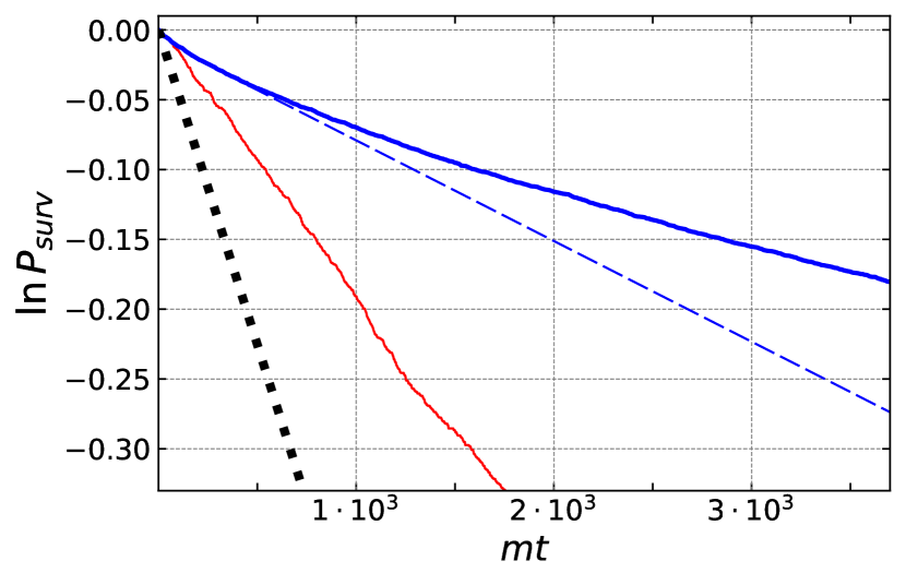
Figure 1: Blue thick: Survival probability in real-time simulations of Hamiltonian dynamics for $\lambda T/m^{3}=0.1$. Blue dashed: Straight line tangent to the previous curve at $t=0$. Red thin: Survival probability from Langevin dynamics (Eq. (13)), at the same temperature and with $\eta=0.01m$. Wiggles in the curve correspond to Poisson fluctuations. Black dotted: Prediction of the Euclidean theory.

Flattening of ${\boldsymbol{\ln}}\,\boldsymbol{P_{surv}}$:‘Classical Zeno effect’ — The measured survival curve in Fig. 1 is not straight: it flattens out as time increases, implying a decrease of the decay rate. The reason for this behavior lies in the dynamics of bubble nucleation. The critical bubble is composed of long modes with wavenumbers $k\lesssim m$, while most of the field energy is stored in shorter modes. The latter provide a thermal bath for the former. However, the energy exchange between different modes is inefficient Boyanovsky et al. (2004). In the model at hand, it is dominated by $2\leftrightarrow 4$ and $3\leftrightarrow 3$ scattering. The corresponding thermalization time is estimated as (see Appendix B),

$$t_{th}\sim\frac{(2\pi)^{3}}{m}\left(\frac{m^{3}}{\lambda T}\right)^{4}\;.$$ (10)

For the temperatures in our simulations $t_{th}\gtrsim 10^{6}/m$ which is longer than the typical decay time $t_{dec}\sim(\Gamma L)^{-1}\sim 10^{4}/m$. The initial power contained in the long modes is then essentially preserved for each individual simulation and controls its lifetime. A simulation which, due to a statistical fluctuation, has a higher long-mode power decays faster, while the one with lower power lives longer.

This, in turn, biases the statistical properties of the surviving ensemble. As the time goes on, the average long-mode power decreases. The effect is apparent in Fig. 2, where we plot the effective temperature of long modes (defined as the variance of their canonical momenta), averaged over the surviving configurations at time $t$. The effective temperature decreases by a few per cent during the run, enough to considerably suppress the bubble nucleation rate. Rather unexpectedly, the decay happens to be non-Markovian: a system that is observed not to decay within a given time has a lower chance of decaying in the future. This is reminiscent of the Zeno effect, which allows one to freeze the evolution of a quantum system by measurements. We stress, however, that in our case, the effect is purely classical.

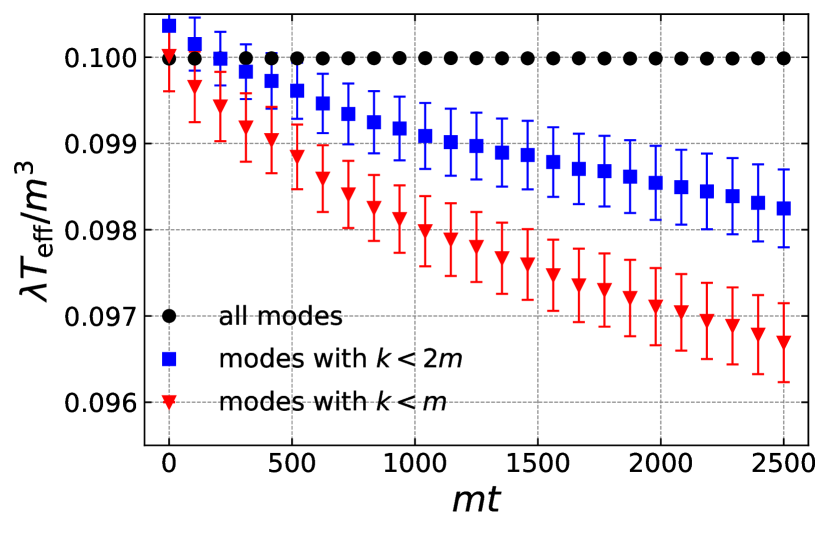
Figure 2: Effective temperature $T_{\rm eff}=\langle|\tilde{\pi}_{j}|^{2}\rangle_{k_{j}<k_{*}}$ of long modes for $k_{*}=m$ and $k_{*}=2m$, averaged over the surviving configurations at time $t$. The temperature computed using all modes is also shown and is time-independent.

The drift in the rate is expected to disappear when the decay is slow enough so that the condition ${t_{dec}\gg t_{th}}$ is satisfied. This condition is likely fulfilled in most cosmological settings. On the other hand, whether it holds in laboratory experiments, especially in those using $(1+1)$-dimensional systems, is less evident. In this case, the classical Zeno effect should be taken into account.

Unbiased rate — For quantitative comparison with the Euclidean prediction (5), we measure the slope $\mathrm{d}\ln P_{surv}/\mathrm{d}t$ at $t\to 0$ corresponding to the rate in the initial unbiased ensemble. We use an extrapolation procedure to increase the accuracy. The probability curve is split into small, approximately linear segments, and the slope of each segment is measured. The logarithms of the slopes thus obtained are fitted with a linear function of time whose value at $t=0$ yields the logarithm of the unbiased rate $\Gamma$. Its error is dominated by statistical uncertainty. Repeating the procedure at different temperatures, we obtain the function $\Gamma(T)$, which we fit by the expression,

$$\ln\Gamma(T)=-\frac{1}{2}\ln T+\ln A-\frac{B}{T}\;,$$ (11)

with free parameters $A$ and $B$. The first term on the right accounts for the temperature dependence of the prefactor predicted by Eq. (5).

First, we eliminate the unknown constant $A$ by taking the ratio $\Gamma(T)/\Gamma(T_{*})$ with $T_{*}$ from the middle of the interval and determine the slope $B$. The fit is shown in the top panel of Fig. 3. It gives $B/E_{b}=0.98\pm 0.02$ with $E_{b}$ from Eq. (5), consistent with the predicted Boltzmann suppression. Note that the bubble energy receives no thermal loop corrections, cf. Alford et al. (1993); Gleiser et al. (1993); Alford and Gleiser (1993).

Next, we measure the prefactor. We fix $B=E_{b}$ in Eq. (11) and extract $A$ at different values of temperature. The ratio of the result to the Euclidean prediction of Eq. (5) is shown in the bottom panel of Fig. 3. The measured prefactor $A^{(sim)}$ is smaller than the prediction $A_{E}$ by a factor $\sim 8$. The ratio is temperature-independent within the error bars. Thus, we can combine the data at different $T$ to obtain

$$A^{(sim)}/A_{E}=0.13\pm 0.01\;.$$ (12)

The discrepancy cannot be attributed to two-loop corrections, which are expected to affect the prefactor only at the $\lambda T/m^{3}\sim 10\%$ level. The independence of the ratio $A^{(sim)}/A_{E}$ of $T$ further rules out this interpretation.

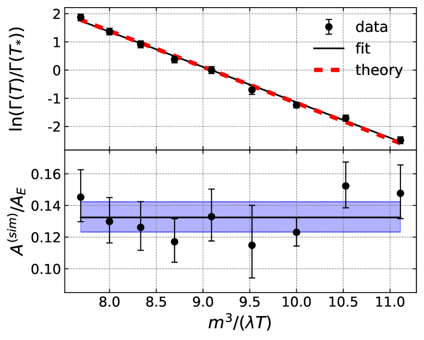
Figure 3: Top: The ratio of unbiased decay rates fitted using Eq. (11). The dashed line is the Euclidean theory prediction. Bottom: Prefactor extracted from real-time simulations $A^{(sim)}$ vs. Euclidean prediction $A_{E}$. The horizontal band shows the average and the corresponding $1\sigma$ error bar.

Decay with an external heat bath — To investigate the system further, we artificially reduce its thermalization time by coupling it to an external heat bath. This is implemented by promoting the equation of motion to the Langevin equation,

$$\ddot{\phi}+\eta\dot{\phi}-\phi^{\prime\prime}+m^{2}\phi-\lambda\phi^{3}=\xi\;,$$ (13)

where $\eta$ is the friction coefficient and $\xi(t,x)$ is the white noise, whose amplitude is fixed by the fluctuation-dissipation theorem:

$$\langle\xi(t,x)\xi(t^{\prime},x^{\prime})\rangle=2\eta T\,\delta(t-t^{\prime})\delta(x-x^{\prime})\,.$$ (14)

We solve this equation numerically using a $3^{\rm rd}$-order stochastic pseudo-spectral operator-splitting scheme Telatovich and Li (2017); Pîrvu et al. (2024). The initial conditions are still set by Eqs. (6) and (7), although we have verified that the evolution becomes insensitive to them after a thermalization time $t_{th}\sim\eta^{-1}$.

We observe that if $\eta\gtrsim 10^{-3}m$ the survival probability curves $\ln P_{surv}(t)$ follow straight lines. This is expected, since now $t_{th}<t_{dec}$ and the classical Zeno effect is absent. However, their slope is still less than the Euclidean prediction, see e.g. the red thin curve in Fig. 1. The measured rate $\Gamma(\eta,T)$ grows as we increase $\eta$ until it reaches a maximum at $\eta\sim 0.3m$ where it deviates from $\Gamma_{E}(T)$ by only $40\%$. At larger $\eta$, it decreases again, consistent with Eq. (2). This behavior is shown in Fig. 4.

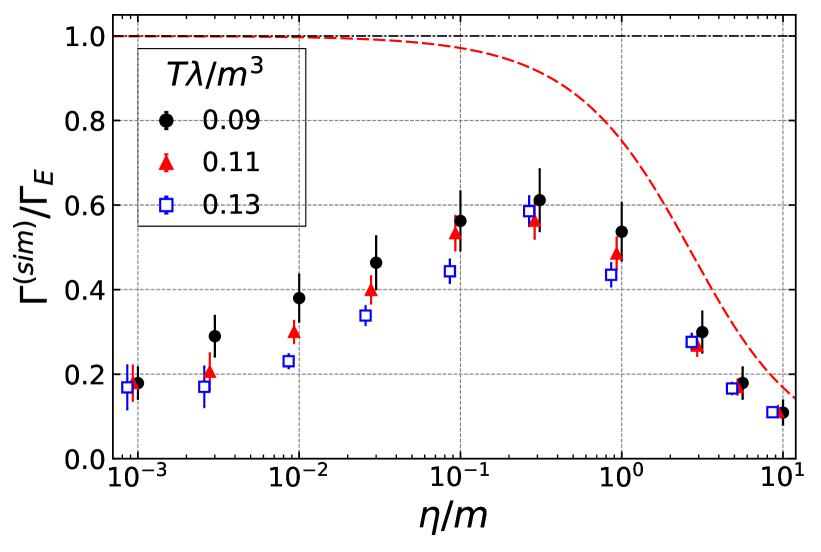
Figure 4: Decay rate measured in simulations as function of the dissipation coefficient $\eta$ for several values of temperature. The rate is normalized by the prediction of Euclidean theory, Eq. (5). The red dashed line shows the prediction of classical statistical theory, Eq. (2).

At $\eta\to 0$, the rate $\Gamma(\eta,T)$ smoothly tends to the value measured in the Hamiltonian system which, as we saw, is significantly lower than $\Gamma_{E}(T)$. To further substantiate this result, we perform the following numerical experiment. We evolve an ensemble of simulations with Eq. (13) for $t\gg\eta^{-1}$, allowing all surviving realizations to reach equilibrium with the heat bath. Then, we abruptly decouple them from the bath by setting $\eta=0$. We find that the survival probability curve exhibits a break upon transitioning from Langevin to Hamiltonian time evolution, as shown in Fig. 5. The final slope is consistent with Eq. (12), confirming that this result does not suffer from any systematics associated with the choice of Gaussian initial conditions (6), (7).

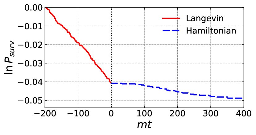
Figure 5: Break in the survival probability curve upon transitioning from Langevin ($\eta=0.1m$) to Hamiltonian ($\eta=0$) evolution at $t=0$. The temperature is $\lambda T/m^{3}=0.1$.

Violation of equilibrium criterion — We see from Fig. 4 that the decay rate is closest to Eq. (2) at $\eta\gtrsim 0.1m$ when the thermalization time is comparable to the inverse mass, and deviates from it at smaller $\eta$ when the thermalization time is longer. This suggests associating the deviation with the lack of thermal equilibrium during the bubble nucleation process, whose dynamical time scale is set by $\omega_{-}=\sqrt{3}m$ (see Eq. (4)). Indeed, in simple mechanical systems with one degree of freedom the applicability of Eq. (2) is known to require Hanggi et al. (1990)

$${\eta/\omega_{-}}>{T/E_{b}}\;,$$ (15)

where $E_{b}$ is the height of the barrier. Otherwise, Eq. (2) overestimates the rate. The condition (15) ensures the Boltzmann distribution in the phase space close to the barrier. One can extend it to multi-dimensional systems, including field theory Pîrvu et al. (2024) where $E_{b}$ coincides with the bubble energy. Note that for fixed $\eta$, the condition (15) is always satisfied at a low enough temperature. Thus, the rate $\Gamma(\eta,T)$ is expected to approach Eq. (2) from below at $T\to 0$ for any $\eta>0$. This is consistent with the trend exhibited by the simulation data in the range $10^{-3}m\lesssim\eta\lesssim 0.1m$ (see Fig. 4), though the measured rate is still far from the limit for the explored temperatures.

The situation is different for the Hamiltonian system with $\eta=0$. In this case, we propose to replace Eq. (15) with a condition on the thermalization time,

$$t_{th}<\frac{E_{b}}{T\omega_{-}}\;.$$ (16)

Comparing with Eq. (10), we see that decreasing the temperature does not help – quite the opposite: the violation of condition (16) becomes stronger as the temperature decreases. This conclusion is not tied to the peculiarities of $(1+1)$-dimensional theory. For example, in classical $\lambda\phi^{4}$ theory in $(3+1)$ dimensions the thermalization time scales as $t_{th}\propto m/(\lambda T)^{2}$, whereas $E_{b}\propto m/\lambda$ and thus Eq. (16) is always violated as long as $T<E_{b}$, i.e. as long as the vacuum decay is exponentially suppressed.

In theories with more than one coupling, e.g. in the presence of additional interacting fields, the condition (16) must be examined case by case. The equilibrium theory is expected to work and Eq. (1) for the rate to be valid only if this condition is fulfilled. Otherwise, Eq. (1) provides an upper bound on the decay rate.

Discussion — The discrepancy between the true rate of thermal false vacuum decay and the Euclidean theory prediction is at the level of the prefactor and may not be important for applications which require only order-of-magnitude estimates. Still, it has deep conceptual implications revealing the non-equilibrium nature of bubble nucleation dynamics. Thermal false vacuum decay turns out not to differ fundamentally from the decay under general non-equilibrium conditions Kofman et al. (1996); Khlebnikov et al. (1998); Gleiser and Howell (2005); Gleiser et al. (2008); Pîrvu et al. (2023); Hiscock (1987); Berezin et al. (1991); Gregory et al. (2014); Tetradis (2016); Gorbunov et al. (2017); Mukaida and Yamada (2017); Kohri and Matsui (2018); Hayashi et al. (2020); Shkerin and Sibiryakov (2021, 2022); Strumia (2023). In the latter case, however, the rate is altered already at the level of the exponential suppression.

Given the inadequacy of the Euclidean approach to the bubble nucleation dynamics, what tools do we have to assess it in the regime of strong exponential suppression, when direct real-time simulations are impractical? One option is provided by the hybrid method of Moore and Rummukainen (2001); Moore et al. (2001) which combines multi-canonical sampling of the thermal ensemble with real-time evolution of configurations with bubbles. It will be interesting to explore if this method captures the non-equilibrium effects found in this work, and if the latter are responsible for the discrepancy with the Euclidean calculation reported recently in Gould et al. (2024). Another option is to adapt the semi-classical methods proposed in Miller (1974); Rubakov et al. (1992); Kuznetsov and Tinyakov (1997); Bonini et al. (1999); Bezrukov et al. (2003); Bezrukov and Levkov (2004); Levkov and Sibiryakov (2005); Levkov et al. (2007, 2009); Demidov and Levkov (2011, 2015a, 2015b); Shkerin and Sibiryakov (2021) for the treatment of dynamical tunneling in non-equilibrium systems. Following this path, one can go beyond classical high-temperature transitions and study vacuum decay in the quantum regime.

Our results do not apply directly to other non-perturbative phenomena, such as sphaleron transitions in the early universe Kuzmin et al. (1985); Rubakov and Shaposhnikov (1996). Unlike false vacuum decay, which is a one-way process, sphaleron transitions can occur in true thermal equilibrium, and, indeed, their rate measured in toy-model real-time simulations was found to agree well with the Euclidean predictions Grigoriev et al. (1989a, b). Nevertheless, our findings strongly motivate revisiting their real-time dynamics, suggesting that it can hide non-equilibrium features.

Acknowledgments — We thank Mustafa Amin, Asimina Arvanitaki, Claudia Cornella, Marco Costa, Ruth Gregory, Junwu Huang, Matthew Johnson, Alexander Kayssi, Juraj Klaric, Andrew Kovachik, Sung-Sik Lee, Alexander Penin, Maxim Pospelov, Jury Radkovski, Kam To Billy Sievers, Mikhail Shaposhnikov and Andrei Zelnikov for fruitful discussions. Research at Perimeter Institute is supported in part by the Government of Canada through the Department of Innovation, Science and Economic Development Canada and by the Province of Ontario through the Ministry of Colleges and Universities. The work of SS is supported by the Natural Sciences and Engineering Research Council (NSERC) of Canada.

Appendix A Euclidean calculation of the decay rate

Here we compute the imaginary part of the false vacuum free energy $F$ entering Eqs. (1), (2) in the model (3). We start with the partition function,

$$\begin{split}Z=\int\![\mathrm{d}\phi]\exp\bigg{\{}-\int\!\mathrm{d}\tau\mathrm{d}x\,\bigg{(}\frac{(\partial_{\mu}\phi)^{2}}{2}+\frac{m^{2}\phi^{2}}{2}-\frac{\lambda\phi^{4}}{4}\bigg{)}\bigg{\}},\end{split}$$ (17)

where the path integral runs over Euclidean configurations with period $1/T$. Besides the vacuum $\phi=0$, the integral has two non-trivial saddle points: the critical bubble $\phi_{b}(x)$ and its reflection $-\phi_{b}(x)$. They correspond to decays towards $\phi=\pm\infty$ and together contribute

$$Z_{b}=2\cdot\bigg{(}\frac{{\cal D}}{{\cal D}^{(0)}}\bigg{)}^{-1/2}\text{e}^{-S[\phi_{b}]}\;.$$ (18)

Here $S[\phi_{b}]=E_{b}/T$ is the bubble action, and ${\cal D}$ is the determinant of small fluctuations around it, normalized by the vacuum determinant ${\cal D}^{(0)}$. It is well-known that ${\cal D}$ is negative due to the presence of the unstable mode, hence the right-hand side of Eq. (18) is imaginary. This gives an imaginary contribution to the free energy,

$$\text{Im}F\equiv-T\,\text{Im}\ln Z=T\cdot 2\cdot\frac{1}{2}\bigg{|}\frac{\mathcal{D}}{\mathcal{D}^{(0)}}\bigg{|}^{-1/2}\text{e}^{-E_{b}/T}\;,$$ (19)

where we have included the factor $1/2$ coming from the integration over the negative mode Coleman (1979).

The determinant ${\cal D}$ is the product over eigenvalues $\alpha_{I}$ of the linearized equation for perturbations:

$$-\Box\varphi_{I}+\big{(}m^{2}-3\lambda\phi_{b}(x)\big{)}\varphi_{I}=\alpha_{I}\,\varphi_{I}\;.$$ (20)

The functions $\varphi_{I}$ are periodic in the Euclidean time. Since the bubble is time-independent, we can separate the variables:

$$\varphi_{I}(\tau,x)=\text{e}^{-i\omega_{n}\tau}\varphi_{n,k}(x)\;,$$ (21)

where $\omega_{n}=2\pi nT$ is the $n^{\rm th}$ Matsubara frequency and the spatial functions satisfy

$${\cal O}(\mu_{n})\,\varphi_{n,k}=\alpha_{n,k}\,\varphi_{n,k}\;,\qquad\mu_{n}^{2}=\omega_{n}^{2}+m^{2}\;,$$ (22)

with the operator

$${\cal O}(\mu)=-\partial^{2}_{x}+\mu^{2}-\frac{6m^{2}}{\mathop{\rm ch}\nolimits^{2}{mx}}\;.$$ (23)

The negative mode lies in the $n=0$ sector and reads:

$$\varphi_{0,0}(x)\propto\frac{1}{\mathop{\rm ch}\nolimits^{2}mx}\;,\qquad\alpha_{0,0}\equiv-\omega_{-}^{2}=-3m^{2}\;.$$ (24)

The determinant ratio factorizes into a product over the Matsubara sectors:

$$\frac{\mathcal{D}}{\mathcal{D}^{(0)}}=\prod_{n=-\infty}^{\infty}\frac{\mathcal{D}_{n}}{\mathcal{D}^{(0)}_{n}}=\frac{\mathcal{D}_{0}}{\mathcal{D}^{(0)}_{0}}\prod_{n=1}^{\infty}\left(\frac{\mathcal{D}_{n}}{\mathcal{D}^{(0)}_{n}}\right)^{2}\;,$$ (25)

where $\mathcal{D}_{n}$ and $\mathcal{D}_{n}^{(0)}$ are determinants of ${\cal O}(\mu_{n})$ and ${\cal O}^{(0)}(\mu_{n})=-\partial_{x}^{2}+\mu_{n}^{2}$, respectively. The product over Matsubara sectors with $n>0$ represents quantum corrections to the prefactor. In the classical (high-temperature) limit this product goes to 1, see Pîrvu et al. (2024) for details, so only the contribution of the $n=0$ sector remains.

It is convenient to compute the determinant of the operator (23) at arbitrary $\mu$. Its ratio to the free determinant with the same $\mu$ is evaluated as Coleman (1979):

$$\frac{\mathcal{D}_{\mu}}{\mathcal{D}_{\mu}^{(0)}}=\lim_{x\to+\infty}\frac{\varphi_{\mu}(x)}{\varphi_{\mu}^{(0)}(x)}\;.$$ (26)

Here $\varphi_{\mu}$, $\varphi_{\mu}^{(0)}$ are solutions of the equations

$${\cal O}(\mu)\varphi_{\mu}(x)=0\;,\qquad{\cal O}^{(0)}(\mu)\varphi_{\mu}^{(0)}=0\;,$$ (27)

with vanishing asymptotics at negative infinity:

$$\varphi_{\mu}=\varphi_{\mu}^{(0)}=\text{e}^{\mu x}\quad\text{at}\quad x\to-\infty\;.$$ (28)

Clearly, $\varphi_{\mu}^{(0)}=\text{e}^{\mu x}$ at all $x$, while $\varphi_{\mu}$ takes the form

$$\varphi_{\mu}(x) =c\,{\rm P}_{2}^{\mu}(x)\;,$$ (29)

$$c =-\mu(1-\mu)(2-\mu)\Gamma(-2-\mu)\;,$$

where ${\rm P}_{2}^{\mu}$ is the associated Legendre polynomial. The asymptotics of (29) at positive infinity reads

$$\varphi_{\mu}(x)=c\,\frac{\text{e}^{\mu x}}{\Gamma(1-\mu)},\quad x\to+\infty\;.$$ (30)

Substituting it into Eq. (26), we obtain

$$\frac{\mathcal{D}_{\mu}}{\mathcal{D}_{\mu}^{(0)}}=\frac{(\mu-m)(\mu-2m)}{(\mu+m)(\mu+2m)}\;.$$ (31)

The determinant in the $n=0$ sector vanishes because the bubble has a translational zero mode

$$\varphi_{0,1}(x)=\sqrt{\frac{3\lambda T}{4m^{3}}}\,\phi_{b}^{\prime}(x)=-\sqrt{\frac{3Tm}{2}}\cdot\frac{\mathop{\rm sh}\nolimits{mx}}{\mathop{\rm ch}\nolimits^{2}{mx}}\;.$$ (32)

The coefficient is fixed by the normalization condition,

$$\int\!\mathrm{d}\tau\,\mathrm{d}x\,\varphi_{0,1}^{2}=1\;.$$ (33)

The zero mode satisfies Eq. (22) with $\mu_{0}=m$ and $\alpha_{0,1}=0$. To regularize the determinant, we take $\mu$ slightly different from $m$. The corresponding operator has a small eigenvalue $\alpha_{0,1}\approx\mu^{2}-m^{2}$. We divide out its contribution and obtain

$$\frac{\mathcal{D}_{0}}{\mathcal{D}^{(0)}_{0}}\mapsto\frac{\mathcal{D}^{\prime}_{0}}{\mathcal{D}^{(0)}_{0}}=\lim_{\mu\to m}\frac{2\pi}{\mu^{2}-m^{2}}\frac{\mathcal{D}_{\mu}}{\mathcal{D}_{\mu}^{(0)}}=-\frac{2\pi}{12m^{2}}\;.$$ (34)

Note that we include a $2\pi$ factor because each mode in the Gaussian integration brings $\sqrt{2\pi/\alpha_{I}}$ with $\alpha_{I}$ being the corresponding eigenvalue.

The integral over the zero mode is replaced by the integral over the positions of the bubble. To this end, we introduce a unity into the path integral (17):

$$\begin{split}1=\int\!\mathrm{d}b\,&\left|\int\!\mathrm{d}\tau\mathrm{d}x\,\phi(\tau,x)\varphi_{0,1}^{\prime}(x+b)\right|\\ &\times\delta\left(\int\!\mathrm{d}\tau\mathrm{d}x\,\phi(\tau,x)\varphi_{0,1}(x+b)\right)\;,\end{split}$$ (35)

and take the integration over $\mathrm{d}b$ outside. The inner integral then runs over configurations orthogonal to ${\varphi_{0,1}(x+b)}$. The saddle point of this integral is given by the shifted bubble $\phi_{b}(x+b)$. Due to the translation invariance, the inner path integral is the same for all $b$, hence the outer integral over $b$ just gives the total length $L$. In addition, we obtain a factor

$$\left|\int\!\mathrm{d}\tau\mathrm{d}x\,\phi_{b}(x)\varphi_{0,1}^{\prime}(x)\right|=\sqrt{\frac{4m^{3}}{3\lambda T}}\;.$$ (36)

Note that the expression inside the square root coincides with the bubble action $S[\phi_{b}]$, as it should be Coleman (1979). Combining Eqs. (34), (36) into the free energy (19) and substituting into Eq. (1) we obtain Eq. (5).

Appendix B Thermalization time

We can estimate the thermalization time by considering the Boltzmann equation for particle phase-space density $f_{p}$, see e.g. Mueller and Son (2004). In $(1+1)$ dimensions the leading processes resulting in the energy exchange between the particles are the $2\leftrightarrow 4$ and $3\leftrightarrow 3$ scatterings which give comparable contributions into the collision integral. For concreteness, let us focus on the former. Denoting the momenta of incoming particles by $p_{1}$, $p_{2}$, we have

$$\begin{split}\frac{\partial f_{p_{1}}}{\partial t}&\simeq\frac{1}{2\omega_{p_{1}}}\int\!\frac{\mathrm{d}\vec{p}_{2}\mathrm{d}\vec{p}_{3}\mathrm{d}\vec{p}_{4}\mathrm{d}\vec{p}_{5}\mathrm{d}\vec{p}_{6}}{(2\pi)^{5}2\omega_{p_{2}}2\omega_{p_{3}}2\omega_{p_{4}}2\omega_{p_{5}}2\omega_{p_{6}}}\\ &\times(2\pi)^{2}\delta^{(2)}(p_{1}+p_{2}-p_{3}-p_{4}-p_{5}-p_{6})|\mathcal{A}_{2\to 4}|^{2}\\ &\times\Bigl{[}-f_{p_{1}}f_{p_{2}}(1+f_{p_{3}})(1+f_{p_{4}})(1+f_{p_{5}})(1+f_{p_{6}})\\ &\qquad+(1+f_{p_{1}})(1+f_{p_{2}})f_{p_{3}}f_{p_{4}}f_{p_{5}}f_{p_{6}}\Bigr{]}\;.\end{split}$$ (37)

Assume for simplicity that all particles have comparable momenta of order $p$. Then the scattering amplitude is $\mathcal{A}_{2\to 4}\sim\lambda^{2}/\omega_{p}^{2}$, and the dominant contribution from the Bose-enhancement factor is $f_{p}^{5}\sim(T/\omega_{p})^{5}$. This yields,

$$\frac{1}{f_{p}}\frac{\partial f_{p}}{\partial t}\sim\frac{1}{(2\pi)^{3}}\frac{\lambda^{4}T^{4}}{\omega_{p}^{11}}\;,$$ (38)

whence we read off the thermalization time

$$t_{th}\sim\frac{(2\pi)^{3}}{m}\left(\frac{m^{3}}{\lambda T}\right)^{4}\left(\frac{\omega_{p}}{m}\right)^{11}\,.$$ (39)

The modes relevant for decay have frequencies $\omega_{p}\sim m$ and thermalize on the time scale (10). Note that the thermalization time grows steeply with the increasing frequency.

Repeating the same argument in $(3+1)$-dimensional theory, where $2\leftrightarrow 2$ processes are relevant, we obtain

$$t_{th}\sim\frac{(2\pi)^{2}}{m}\left(\frac{m}{\lambda T}\right)^{2}\left(\frac{\omega_{p}}{m}\right)\;.$$ (40)

In this case the thermalization time scales as the inverse square of the temperature.

References

- Onuki (2002) Akira Onuki, Phase Transition Dynamics (Cambridge University Press, 2002).
- Quiros (1999) Mariano Quiros, “Finite temperature field theory and phase transitions,” in ICTP Summer School in High-Energy Physics and Cosmology (1999) pp. 187–259, arXiv:hep-ph/9901312 .
- Bodeker and Buchmuller (2021) Dietrich Bodeker and Wilfried Buchmuller, “Baryogenesis from the weak scale to the grand unification scale,” Rev. Mod. Phys. 93, 035004 (2021), arXiv:2009.07294 [hep-ph] .
- Caprini and Figueroa (2018) Chiara Caprini and Daniel G. Figueroa, “Cosmological Backgrounds of Gravitational Waves,” Class. Quant. Grav. 35, 163001 (2018), arXiv:1801.04268 [astro-ph.CO] .
- Caprini et al. (2020) Chiara Caprini et al., “Detecting gravitational waves from cosmological phase transitions with LISA: an update,” JCAP 03, 024 (2020), arXiv:1910.13125 [astro-ph.CO] .
- Buttazzo et al. (2013) Dario Buttazzo, Giuseppe Degrassi, Pier Paolo Giardino, Gian F. Giudice, Filippo Sala, Alberto Salvio, and Alessandro Strumia, “Investigating the near-criticality of the Higgs boson,” JHEP 12, 089 (2013), arXiv:1307.3536 [hep-ph] .
- Bednyakov et al. (2015) A. V. Bednyakov, B. A. Kniehl, A. F. Pikelner, and O. L. Veretin, “Stability of the Electroweak Vacuum: Gauge Independence and Advanced Precision,” Phys. Rev. Lett. 115, 201802 (2015), arXiv:1507.08833 [hep-ph] .
- Fialko et al. (2015) O. Fialko, B. Opanchuk, A. I. Sidorov, P. D. Drummond, and J. Brand, “Fate of the false vacuum: towards realization with ultra-cold atoms,” EPL 110, 56001 (2015), arXiv:1408.1163 [cond-mat.quant-gas] .
- Fialko et al. (2017) Oleksandr Fialko, Bogdan Opanchuk, Andrei I. Sidorov, Peter D. Drummond, and Joachim Brand, “The universe on a table top: engineering quantum decay of a relativistic scalar field from a metastable vacuum,” J. Phys. B 50, 024003 (2017), arXiv:1607.01460 [cond-mat.quant-gas] .
- Braden et al. (2018) Jonathan Braden, Matthew C. Johnson, Hiranya V. Peiris, and Silke Weinfurtner, “Towards the cold atom analog false vacuum,” JHEP 07, 014 (2018), arXiv:1712.02356 [hep-th] .
- Billam et al. (2019) Thomas P. Billam, Ruth Gregory, Florent Michel, and Ian G. Moss, “Simulating seeded vacuum decay in a cold atom system,” Phys. Rev. D 100, 065016 (2019), arXiv:1811.09169 [hep-th] .
- Braden et al. (2019a) Jonathan Braden, Matthew C. Johnson, Hiranya V. Peiris, Andrew Pontzen, and Silke Weinfurtner, “Nonlinear Dynamics of the Cold Atom Analog False Vacuum,” JHEP 10, 174 (2019a), arXiv:1904.07873 [hep-th] .
- Billam et al. (2022) Thomas P. Billam, Kate Brown, and Ian G. Moss, “False-vacuum decay in an ultracold spin-1 Bose gas,” Phys. Rev. A 105, L041301 (2022), arXiv:2108.05740 [cond-mat.quant-gas] .
- Jenkins et al. (2024) Alexander C. Jenkins, Jonathan Braden, Hiranya V. Peiris, Andrew Pontzen, Matthew C. Johnson, and Silke Weinfurtner, “Analog vacuum decay from vacuum initial conditions,” Phys. Rev. D 109, 023506 (2024), arXiv:2307.02549 [cond-mat.quant-gas] .
- Jenkins et al. (2023) Alexander C. Jenkins, Ian G. Moss, Thomas P. Billam, Zoran Hadzibabic, Hiranya V. Peiris, and Andrew Pontzen, “Generalized cold-atom simulators for vacuum decay,” (2023), arXiv:2311.02156 [cond-mat.quant-gas] .
- Zenesini et al. (2024) Alessandro Zenesini, Anna Berti, Riccardo Cominotti, Chiara Rogora, Ian G. Moss, Thomas P. Billam, Iacopo Carusotto, Giacomo Lamporesi, Alessio Recati, and Gabriele Ferrari, “False vacuum decay via bubble formation in ferromagnetic superfluids,” Nature Phys. 20, 558–563 (2024), arXiv:2305.05225 [hep-ph] .
- Kobzarev et al. (1974) I. Yu. Kobzarev, L. B. Okun, and M. B. Voloshin, “Bubbles in Metastable Vacuum,” Yad. Fiz. 20, 1229–1234 (1974).
- Coleman (1977) Sidney R. Coleman, “The Fate of the False Vacuum. 1. Semiclassical Theory,” Phys. Rev. D 15, 2929–2936 (1977), [Erratum: Phys.Rev.D 16, 1248 (1977)].
- Callan and Coleman (1977) Curtis G. Callan, Jr. and Sidney R. Coleman, “The Fate of the False Vacuum. 2. First Quantum Corrections,” Phys. Rev. D 16, 1762–1768 (1977).
- Linde (1981) Andrei D. Linde, “Fate of the False Vacuum at Finite Temperature: Theory and Applications,” Phys. Lett. 100B, 37–40 (1981).
- Linde (1983) Andrei D. Linde, “Decay of the False Vacuum at Finite Temperature,” Nucl. Phys. B 216, 421 (1983), [Erratum: Nucl.Phys.B 223, 544 (1983)].
- Affleck (1981) Ian Affleck, “Quantum Statistical Metastability,” Phys. Rev. Lett. 46, 388 (1981).
- Weinberg (2012) Erick J. Weinberg, Classical solutions in quantum field theory: Solitons and Instantons in High Energy Physics, Cambridge Monographs on Mathematical Physics (Cambridge University Press, 2012).
- Langer (1969) J. S. Langer, “Statistical theory of the decay of metastable states,” Annals Phys. 54, 258–275 (1969).
- Hanggi et al. (1990) Peter Hanggi, Peter Talkner, and Michal Borkovec, “Reaction-Rate Theory: Fifty Years After Kramers,” Rev. Mod. Phys. 62, 251–341 (1990).
- Grigoriev and Rubakov (1988) Dmitri Yu. Grigoriev and V. A. Rubakov, “Soliton Pair Creation at Finite Temperatures. Numerical Study in (1+1)-dimensions,” Nucl. Phys. B 299, 67–78 (1988).
- Grigoriev et al. (1989a) Dmitri Yu. Grigoriev, V. A. Rubakov, and M. E. Shaposhnikov, “Sphaleron Transitions at Finite Temperatures: Numerical Study in (1+1)-dimensions,” Phys. Lett. B 216, 172–176 (1989a).
- Grigoriev et al. (1989b) Dmitri Yu. Grigoriev, V. A. Rubakov, and M. E. Shaposhnikov, “Topological Transitions at Finite Temperatures: A Real Time Numerical Approach,” Nucl. Phys. B 326, 737–757 (1989b).
- Ambjorn et al. (1990) Jan Ambjorn, T. Askgaard, H. Porter, and M. E. Shaposhnikov, “Lattice Simulations of Electroweak Sphaleron Transitions in Real Time,” Phys. Lett. B 244, 479–487 (1990).
- Valls and Mazenko (1990) Oriol T. Valls and Gene F. Mazenko, “Nucleation in a time-dependent Ginzburg-Landau model: A numerical study,” Phys. Rev. B 42, 6614–6622 (1990).
- Alford et al. (1992) Mark G. Alford, Hume Feldman, and Marcelo Gleiser, “Thermal nucleation of kink - anti-kink pairs,” Phys. Rev. Lett. 68, 1645–1648 (1992).
- Alford et al. (1993) Mark G. Alford, H. Feldman, and M. Gleiser, “Thermal activation of metastable decay: Testing nucleation theory,” Phys. Rev. D 47, R2168–R2171 (1993).
- Alford and Gleiser (1993) Mark G. Alford and Marcelo Gleiser, “Metastability in two-dimensions and the effective potential,” Phys. Rev. D 48, 2838–2844 (1993), arXiv:hep-ph/9304245 .
- Borsanyi et al. (2000) Sz. Borsanyi, A. Patkos, J. Polonyi, and Zs. Szep, “Fate of the classical false vacuum,” Phys. Rev. D 62, 085013 (2000), arXiv:hep-th/0004059 .
- Braden et al. (2019b) Jonathan Braden, Matthew C. Johnson, Hiranya V. Peiris, Andrew Pontzen, and Silke Weinfurtner, “New Semiclassical Picture of Vacuum Decay,” Phys. Rev. Lett. 123, 031601 (2019b), [Erratum: Phys.Rev.Lett. 129, 059901 (2022)], arXiv:1806.06069 [hep-th] .
- Batini et al. (2024) Laura Batini, Aleksandr Chatrchyan, and Jürgen Berges, “Real-time dynamics of false vacuum decay,” Phys. Rev. D 109, 023502 (2024), arXiv:2310.04206 [hep-th] .
- Aguirre et al. (2012) Anthony Aguirre, Sean M. Carroll, and Matthew C. Johnson, “Out of equilibrium: understanding cosmological evolution to lower-entropy states,” JCAP 02, 024 (2012), arXiv:1108.0417 [hep-th] .
- Gleiser et al. (1991) Marcelo Gleiser, Edward W. Kolb, and Richard Watkins, “Phase transitions with subcritical bubbles,” Nucl. Phys. B 364, 411–450 (1991).
- Gleiser and Howell (2005) Marcelo Gleiser and Rafael C. Howell, “Resonant nucleation,” Phys. Rev. Lett. 94, 151601 (2005), arXiv:hep-ph/0409179 .
- Gleiser et al. (2008) Marcelo Gleiser, Barrett Rogers, and Joel Thorarinson, “Bubbling the False Vacuum Away,” Phys. Rev. D 77, 023513 (2008), arXiv:0708.3844 [hep-th] .
- Pîrvu et al. (2023) Dalila Pîrvu, Matthew C. Johnson, and Sergey Sibiryakov, “Bubble velocities and oscillon precursors in first order phase transitions,” (2023), arXiv:2312.13364 [hep-th] .
- Pîrvu et al. (2024) D. Pîrvu, A. Shkerin, and S. Sibiryakov, (2024), in preparation.
- Boyanovsky et al. (2004) D. Boyanovsky, C. Destri, and H. J. de Vega, “The Approach to thermalization in the classical theory in (1+1)-dimensions: Energy cascades and universal scaling,” Phys. Rev. D 69, 045003 (2004), arXiv:hep-ph/0306124 .
- Gleiser et al. (1993) Marcelo Gleiser, Gil C. Marques, and Rudnei O. Ramos, “On the evaluation of thermal corrections to false vacuum decay rates,” Phys. Rev. D 48, 1571–1584 (1993), arXiv:hep-ph/9304234 .
- Telatovich and Li (2017) Adam Telatovich and Xiantao Li, “The strong convergence of operator-splitting methods for the langevin dynamics model,” (2017), arXiv:1706.04237 .
- Kofman et al. (1996) Lev Kofman, Andrei D. Linde, and Alexei A. Starobinsky, “Nonthermal phase transitions after inflation,” Phys. Rev. Lett. 76, 1011–1014 (1996), arXiv:hep-th/9510119 .
- Khlebnikov et al. (1998) S. Khlebnikov, L. Kofman, Andrei D. Linde, and I. Tkachev, “First order nonthermal phase transition after preheating,” Phys. Rev. Lett. 81, 2012–2015 (1998), arXiv:hep-ph/9804425 .
- Hiscock (1987) W. A. Hiscock, “Can black holes nucleate vacuum phase transitions?” Phys. Rev. D 35, 1161–1170 (1987).
- Berezin et al. (1991) V. A. Berezin, V. A. Kuzmin, and I. I. Tkachev, “Black holes initiate false vacuum decay,” Phys. Rev. D 43, 3112–3116 (1991).
- Gregory et al. (2014) Ruth Gregory, Ian G. Moss, and Benjamin Withers, “Black holes as bubble nucleation sites,” JHEP 03, 081 (2014), arXiv:1401.0017 [hep-th] .
- Tetradis (2016) Nikolaos Tetradis, “Black holes and Higgs stability,” JCAP 09, 036 (2016), arXiv:1606.04018 [hep-ph] .
- Gorbunov et al. (2017) Dmitry Gorbunov, Dmitry Levkov, and Alexander Panin, “Fatal youth of the Universe: black hole threat for the electroweak vacuum during preheating,” JCAP 10, 016 (2017), arXiv:1704.05399 [astro-ph.CO] .
- Mukaida and Yamada (2017) Kyohei Mukaida and Masaki Yamada, “False Vacuum Decay Catalyzed by Black Holes,” Phys. Rev. D 96, 103514 (2017), arXiv:1706.04523 [hep-th] .
- Kohri and Matsui (2018) Kazunori Kohri and Hiroki Matsui, “Electroweak Vacuum Collapse induced by Vacuum Fluctuations of the Higgs Field around Evaporating Black Holes,” Phys. Rev. D 98, 123509 (2018), arXiv:1708.02138 [hep-ph] .
- Hayashi et al. (2020) Takumi Hayashi, Kohei Kamada, Naritaka Oshita, and Jun’ichi Yokoyama, “On catalyzed vacuum decay around a radiating black hole and the crisis of the electroweak vacuum,” JHEP 08, 088 (2020), arXiv:2005.12808 [hep-th] .
- Shkerin and Sibiryakov (2021) Andrey Shkerin and Sergey Sibiryakov, “Black hole induced false vacuum decay from first principles,” JHEP 11, 197 (2021), arXiv:2105.09331 [hep-th] .
- Shkerin and Sibiryakov (2022) Andrey Shkerin and Sergey Sibiryakov, “Black hole induced false vacuum decay: the role of greybody factors,” JHEP 08, 161 (2022), arXiv:2111.08017 [hep-th] .
- Strumia (2023) Alessandro Strumia, “Black holes don’t source fast Higgs vacuum decay,” JHEP 03, 039 (2023), arXiv:2209.05504 [hep-ph] .
- Moore and Rummukainen (2001) Guy D. Moore and Kari Rummukainen, “Electroweak bubble nucleation, nonperturbatively,” Phys. Rev. D 63, 045002 (2001), arXiv:hep-ph/0009132 .
- Moore et al. (2001) Guy D. Moore, Kari Rummukainen, and Anders Tranberg, “Nonperturbative computation of the bubble nucleation rate in the cubic anisotropy model,” JHEP 04, 017 (2001), arXiv:hep-lat/0103036 .
- Gould et al. (2024) Oliver Gould, Anna Kormu, and David J. Weir, “A nonperturbative test of nucleation calculations for strong phase transitions,” (2024), arXiv:2404.01876 [hep-th] .
- Miller (1974) William H Miller, “Classical-limit quantum mechanics and the theory of molecular collisions,” Advances in chemical physics , 69–177 (1974).
- Rubakov et al. (1992) V. A. Rubakov, D. T. Son, and P. G. Tinyakov, “Classical boundary value problem for instanton transitions at high-energies,” Phys. Lett. B 287, 342–348 (1992).
- Kuznetsov and Tinyakov (1997) A. N. Kuznetsov and P. G. Tinyakov, “False vacuum decay induced by particle collisions,” Phys. Rev. D 56, 1156–1169 (1997), arXiv:hep-ph/9703256 .
- Bonini et al. (1999) G. F. Bonini, Andrew G. Cohen, C. Rebbi, and V. A. Rubakov, “The Semiclassical description of tunneling in scattering with multiple degrees of freedom,” Phys. Rev. D 60, 076004 (1999), arXiv:hep-ph/9901226 .
- Bezrukov et al. (2003) F. L. Bezrukov, D. Levkov, C. Rebbi, V. A. Rubakov, and P. Tinyakov, “Semiclassical study of baryon and lepton number violation in high-energy electroweak collisions,” Phys. Rev. D 68, 036005 (2003), arXiv:hep-ph/0304180 .
- Bezrukov and Levkov (2004) F. L. Bezrukov and D. Levkov, “Dynamical tunneling of bound systems through a potential barrier: complex way to the top,” J. Exp. Theor. Phys. 98, 820–836 (2004), arXiv:quant-ph/0312144 .
- Levkov and Sibiryakov (2005) D. Levkov and S. Sibiryakov, “Real-time instantons and suppression of collision-induced tunneling,” JETP Lett. 81, 53–57 (2005), arXiv:hep-th/0412253 .
- Levkov et al. (2007) D. G. Levkov, A. G. Panin, and S. M. Sibiryakov, “Unstable Semiclassical Trajectories in Tunneling,” Phys. Rev. Lett. 99, 170407 (2007), arXiv:0707.0433 [quant-ph] .
- Levkov et al. (2009) D. G. Levkov, A. G. Panin, and S. M. Sibiryakov, “Signatures of unstable semiclassical trajectories in tunneling,” J. Phys. A 42, 205102 (2009), arXiv:0811.3391 [quant-ph] .
- Demidov and Levkov (2011) S. V. Demidov and D. G. Levkov, “Soliton-antisoliton pair production in particle collisions,” Phys. Rev. Lett. 107, 071601 (2011), arXiv:1103.0013 [hep-th] .
- Demidov and Levkov (2015a) Sergei Demidov and Dmitry Levkov, “High-energy limit of collision-induced false vacuum decay,” JHEP 06, 123 (2015a), arXiv:1503.06339 [hep-ph] .
- Demidov and Levkov (2015b) S. V. Demidov and D. G. Levkov, “Semiclassical description of soliton-antisoliton pair production in particle collisions,” JHEP 11, 066 (2015b), arXiv:1509.07125 [hep-th] .
- Kuzmin et al. (1985) V. A. Kuzmin, V. A. Rubakov, and M. E. Shaposhnikov, “On the Anomalous Electroweak Baryon Number Nonconservation in the Early Universe,” Phys. Lett. B 155, 36 (1985).
- Rubakov and Shaposhnikov (1996) V. A. Rubakov and M. E. Shaposhnikov, “Electroweak baryon number nonconservation in the early universe and in high-energy collisions,” Usp. Fiz. Nauk 166, 493–537 (1996), arXiv:hep-ph/9603208 .
- Coleman (1979) Sidney R. Coleman, “The Uses of Instantons,” Subnucl. Ser. 15, 805 (1979).
- Mueller and Son (2004) A. H. Mueller and D. T. Son, “On the Equivalence between the Boltzmann equation and classical field theory at large occupation numbers,” Phys. Lett. B 582, 279–287 (2004), arXiv:hep-ph/0212198 .