Classical relativistic nonholonomic mechanics and time-dependent $G$-Chaplygin systems with affine constraints

Abstract.

We study the relativistic formulation of a classical time-dependent nonholonomic Lagrangian mechanics from the perspective of moving frames. We also introduce time-dependent $G$-Chaplygin systems with affine constraints, which are natural objects for the invariant formulation of nonholonomic systems with symmetries. As far as the author is aware, the Hamiltonization problem for time-dependent constraints has not yet been studied. As a first step in this direction, we consider a rolling without sliding of a balanced disc of radius $r$ over a vertical circle of variable radius $R(t)$. We modify the Chaplygin multiplier method and prove that the reduced system becomes the usual Lagrangian system with respect to the new time.

1. Introduction

Galileo Galilei’s (1564–1642) principle of relativity is one of the most important steps towards understanding nature. In modern terms it was formulated by Poincaré, see e.g. [34] (we follow Arnold [1]):

• All the laws of nature at all moments of time are the same in all inertial coordinate systems.

• A coordinate system in uniform rectilinear motion with respect to an inertial one is also inertial.

Depending on the geometric structure of the 4-dimensional affine space-time, we obtain two different mechanics: classical and special relativity, which share the same Galilean principle of relativity (see e.g. [1, 25]).

We study the relativistic formulation of a classical time-dependent nonholonomic Lagrangian mechanics. We follow [26] where we have treated holonomic systems. It appears that for a space-time formulation of nonholonomic mechanics it is natural to pass from a class of systems with homogeneous nonholonomic constraints defined by distributions of the tangent bundle of the configuration space to a class of nonholonomic systems with nonhomogeneous constraints. That is why we consider a constrained Lagrangian system $(Q,L,\mathcal{A})$, where $Q$ is an $n$–dimensional configuration space, $L\colon TQ\times\mathbb{R}\to\mathbb{R}$ is a time-dependent Lagrangian and a motion is subject to time-dependent non-homogeneous constraints: the velocity $\dot{\gamma}(t)$ of an admissible motion $\gamma(t)$ belongs to a time-dependent affine distribution $\mathcal{A}_{t}$ of the tangent bundle $TQ$. A motion of the system is derived from the d’Alambert principle or the d’Alambert-Lagrange principle: the trajectories of a mechanical system are obtained from the condition that the variational derivative of the Lagrangian vanishes along virtual displacements [2, 8].

Note that the d’Alambert principle in classical Lagrangian mechanics fulfils the following general variant of the principle of relativity, which does not include a notion of inertial frames (see e.g. [26]):

• All the laws of nature at all moments of time are the same in all reference frames.

With appropriate geometric structures on space-time manifolds and a notion of reference frame, both general relativity (with local meaning of time and reference frame) and classical mechanics agree with the above principle. The invariant formulation of classical nonholonomic Lagrangian mechanics on a space-time manifold is well known (see e.g. [31] and references therein), but is not so emphasised. On the other hand, the above principle, incorporated in Einstein’s general equivalence principle, was one of the basic motivations for its foundation, and it is widely used in general relativity.

Here we have presented the space-time formulation of nonholonomic mechanics by using analogies to fixed and moving reference frames in rigid body dynamics. We also introduce time-dependent $G$-Chaplygin systems with affine constraints, which are natural objects for the invariant formulation of nonholonomic systems with symmetries.

1.1. Outline and results of the paper

In section 2 we recall the d’Alambert principle for a nonholonomic Lagrangian system $(Q,L,\mathcal{A})$, which also includes the field of non-potential forces $\mathbf{F}$. Motivated by the notion of fixed and moving reference frames in rigid body dynamics [1, 2, 26], we consider arbitrary time-dependent transformations between the configuration space $Q$ (the fixed reference frame) and the manifold $M$ diffeomorphic to $Q$ (the moving reference frame) and consider trajectories of a nonholonomic Lagrangian system in both reference frames (Theorem 3.1). A notion of moving energy [11, 19] naturally appears in the relativistic formulation of nonholonomic mechanics (section 3). All considerations are valid without the assumption that the Lagrangian is regular and are derived without the use of Lagrange multipliers.

In section 4 we apply the construction of moving reference frames for the invariant formulation of nanholonomic Lagrangian mechanics in a space-time, $(n+1)$–dimensional manifold $\mathcal{Q}$, which is fibred over $\mathbb{R}$ with fibers diffeomorphic to $Q$. The invariant formulation of time-dependent classical Lagrangian mechanics is well studied (see e.g. [31] and references therein). Here, following [26], we have tried to present it with minimal technical requirements.

In section 5 we consider nonholonomic systems $(Q,L,\mathcal{A})$ on fiber spaces and in Section 6 we use them to describe the reduction of time-dependent $G$–Chaplygin systems associated to time-dependent principal bundles. Recall that the usual $G$–Chaplygin systems have a natural geometric framework as connections on principal bundles (see [29, 18]). On the other hand, nonholonomic systems with symmetries, in particular Chaplygin systems, are incorporated into the geometric framework of Ehresmann connections on fiber spaces (see [9]). In this paper, following [17], we combine the approach of [9] with the Voronec nonholonomic equations [35] and derive an invariant form of the Voronec equations for time-dependent Ehresmann connections (Theorem 5.1, Proposition 5.1). The invariant form of the equations allows us to perform a $G$–Chaplygin reduction for the case of non-Abelian time-dependent symmetries (Theorem 6.1).

A naturally related problem is the Hamiltonization of $G$–Chaplygin systems. For natural mechanical systems, the reduced system has more additional terms compared to the usual case of homogeneous time-independent constraints (see section 6). As far as the author is aware, the Hamiltonization problem for time-dependent constraints has not yet been studied. As a first step in this direction, we consider a rolling without sliding of a balanced disc of radius $r$ over a vertical circle of variable radius $R(t)$. We modify the Chaplygin multiplier method and prove that the reduced system becomes the usual Lagrangian system with respect to the new time (Theorem 6.2).

2. D’Alambert principle

2.1. Nonholonomic systems with affine constraints

We consider a nonholonomic Lagrangian system $(Q,L,\mathcal{A})$, where $Q$ is an $n$–dimensional configuration space, $L(q,\dot{q},t)$ is a time–dependent Lagrangian, $L:TQ\times\mathbb{R}\to\mathbb{R}$, and $\mathcal{A}$ are nonholonomic constraints

$$\mathcal{A}=\{(\mathcal{A}_{t},t)\,|\,t\in\mathbb{R}\}\subset TQ\times\mathbb{R},$$

where $\mathcal{A}_{t}$ is a time-dependent affine distribution of rank $m$ of the tangent bundle $TQ$. A curve $\gamma\colon\mathbb{R}\to Q$ is admissible (or allowed by constraints) if the velocity $\dot{\gamma}(t)$ belongs to $\mathcal{A}_{t}$, $t\in\mathbb{R}$.

The affine distribution can be written in the following form

$$\mathcal{A}_{t}=\mathcal{D}_{t}+\chi_{t},$$

where $\mathcal{D}_{t}$ is a time-dependent distribution of rank $m$ and $\chi_{t}$ is a time-dependent vector field on $Q$ defined modulo $\mathcal{D}_{t}$. The vectors in $\mathcal{A}_{t}$ are called admissible velocities, while the vectors in $\mathcal{D}_{t}$ are called virtual displacements.

Let $r=n-m$. In local coordinates $q=(q^{1},\dots,q^{n})$ on $Q$, the constraints are given by equations

(2.1) $$\dot{q}\in\mathcal{A}_{t}|_{q}\Longleftrightarrow\sum_{i=1}^{n}a_{\nu i}(q,t)\dot{q}^{i}+a_{\nu}(q,t)=0,\qquad\nu=1,\dots,r,$$

while virtual displacements satisfy

$$\eta\in\mathcal{D}_{t}|_{q}\Longleftrightarrow\sum_{i=1}^{n}a_{\nu i}(q,t)\eta^{i}=0,\qquad\nu=1,\dots,r,$$

where $\operatorname{\mathrm{rank}}(a_{\nu i})_{1\leq\nu\leq r,1\leq i\leq n}=r$.

We assume that the constraints are nonholonomic. This means that there are no functions $f_{\nu}(q^{1},\dots,q^{n},t)$, $\nu=1,\dots,r$, such that the affine distribution $\mathcal{A}_{t}$ is locally defined by (2.1), where

$$a_{\nu}=\frac{\partial f_{\alpha}}{\partial t},\qquad a_{\nu i}=\frac{\partial f_{\nu}}{\partial q^{i}},\qquad\nu=1,\dots,r,\qquad i=1,\dots,n.$$

That is why it is convenient to consider the rank $(m+1)$ distribution $\underline{\mathcal{A}}\subset T(Q\times\mathbb{R})$ of the extended configuration space $Q\times\mathbb{R}$ defined by

(2.2) $$\underline{\mathcal{A}}_{(q,t)}=\big{\{}\lambda\eta+\mu\big{(}\chi_{t}+\frac{\partial}{\partial t}\big{)}\,\big{|}\,\eta\in\mathcal{D}_{t}|_{q},\lambda,\mu\in\mathbb{R}\big{\}}\subset T_{(q,t)}(Q\times\mathbb{R}),$$

or in local coordinates

$$\underline{\eta}=\sum_{i=1}^{n}\eta^{i}\frac{\partial}{\partial q^{i}}+\eta_{t}\frac{\partial}{\partial t}\in\underline{\mathcal{A}}_{(q,t)}\Longleftrightarrow\sum_{i=1}^{n}a_{\nu i}(q,t)\eta^{i}+a_{\nu}(q,t)\eta_{t}=0,\qquad\nu=1,\dots,r.$$

According to the Frobenious theorem, if $\underline{\mathcal{A}}$ is nonintegrable, the constraints are nonholonomic.

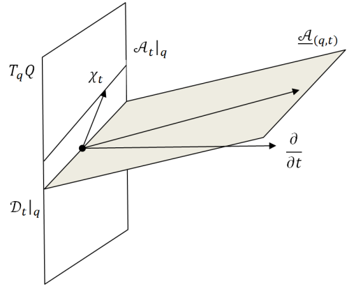
Figure 1. The tangent space $T_{(q,t)}(Q\times\mathbb{R})$ of the extended configuration space and its subspaces $\mathcal{D}_{t}|_{q},\mathcal{A}_{t}|_{q}\subset T_{q}Q$ and $\underline{\mathcal{A}}_{(q,t)}$.

Example 2.1.

Consider $Q=\mathbb{R}^{2}\{x,y\}$ and the nonhomogeneous constraint

(2.3) $$\dot{x}-a(x,y,t)\dot{y}-b(x,y,t)=0.$$

Then

$${\mathcal{D}}_{t}|_{(x,y)}=\big{\{}\xi=\xi_{x}\frac{\partial}{\partial x}+\xi_{y}\frac{\partial}{\partial y}\in T_{(x,y)}\mathbb{R}^{2}\,\big{|}\,\xi_{x}=a(x,y,t)\xi_{y}\big{\}},\quad\chi_{t}=b(x,y,t)\frac{\partial}{\partial x}$$

$${\mathcal{A}}_{t}|_{(x,y)}=\big{\{}\xi=\xi_{x}\frac{\partial}{\partial x}+\xi_{y}\frac{\partial}{\partial y}\in T_{(x,y)}\mathbb{R}^{2}\,\big{|}\,\xi_{x}=a(x,y,t)\xi_{y}+b(x,y,t)\big{\}},$$

$$\underline{\mathcal{A}}_{(x,y,t)}=\big{\{}\xi_{x}\frac{\partial}{\partial x}+\xi_{y}\frac{\partial}{\partial y}+\xi_{t}\frac{\partial}{\partial t}\in T_{(x,y,t)}\mathbb{R}^{3}\,\big{|}\,\xi_{x}=a(x,y,t)\xi_{y}+b(x,y,t)\xi_{t}\big{\}}$$

Since $\underline{\mathcal{A}}$ is a kernel of 1-form $\alpha=dx-ady-bdt$ on the extended configuration space $\mathbb{R}^{3}\{(x,y,t)\}$, the constraint (2.3) is nonholonomic if $\alpha$ is a contact:

$$\alpha\wedge d\alpha= \big{(}dx-ady-bdt\big{)}\wedge\big{(}\frac{\partial a}{\partial t}dy\wedge dt-\frac{\partial a}{\partial x}dx\wedge dy-\frac{\partial b}{\partial y}dy\wedge dt-\frac{\partial b}{\partial x}dx\wedge dt\big{)}$$

$$= \big{(}\frac{\partial a}{\partial t}-\frac{\partial b}{\partial y}+b\frac{\partial a}{\partial x}-a\frac{\partial b}{\partial x}\big{)}dx\wedge dy\wedge dt\neq 0,$$

In particular, even for homogeneous constraints $b\equiv 0$, if ${\partial a}/{\partial t}\neq 0$ the constraints are nonholonomic, although the distribution $\mathcal{A}_{t}=\mathcal{D}_{t}$ is integrable for any fixed $t$.

2.2. Dynamics

In classical mechanics, the dynamics in the case of ideal nonholonomic constraints is defined by the d’Alembert principle (e.g, see [2, 8]): an admissible curve $\gamma$ is a motion of the constrained Lagrangian system $(Q,L,\mathcal{A})$ if the variational derivative $\delta L(\eta)|_{\gamma}$ vanishes for all virtual displacements $\eta$ along $\gamma$:

$$\delta L(\eta)|_{\gamma}=\sum_{i=1}^{n}\big{(}\frac{\partial L}{\partial q^{i}}-\frac{d}{dt}\frac{\partial L}{\partial\dot{q}^{i}}\big{)}\eta^{i}|_{\gamma(t)}=0,\qquad\eta|_{\gamma(t)}\in\mathcal{D}_{t}|_{\gamma(t)}.$$

For integrable constraints, the principle is equivalent to another fundamental principle – Hamiltonian principle of least action, see e.g. [2, 8, 26].

If we also have a field of non-potential forces $\mathbf{F}(q,\dot{q},t)$,

$$\mathbf{F}(q,\dot{q},t)=\sum_{i=1}^{n}F_{i}(q,\dot{q},t)dq^{i},$$

the equations of motion are given by

(2.4) $$\delta L(\eta)|_{\gamma}+\mathbf{F}(\eta)|_{\gamma}=\sum_{i=1}^{n}\big{(}\frac{\partial L}{\partial q^{i}}-\frac{d}{dt}\frac{\partial L}{\partial\dot{q}^{i}}+F_{i}\big{)}\eta^{i}|_{\gamma(t)}=0,\qquad\eta|_{\gamma(t)}\in\mathcal{D}_{t}|_{\gamma(t)}.$$

Consider the associated time-dependent fiber derivative $\mathbb{F}L:TQ\to T^{*}Q$ defined by

(2.5) $$\mathbb{F}L(q,\xi,t)(\eta)=\frac{d}{ds}|_{s=0}L(q,\xi+s\eta,t),\qquad\xi,\eta\in T_{q}Q.$$

If (2.5) is a diffeomorphism between $TQ$ and $T^{*}Q$ for all $t\in\mathbb{R}$, the corresponding Lagrangian $L$ is called regular. Then the initial value problem $q(t_{0})=q_{0}$, $\dot{q}(t_{0})=\dot{q}_{0}$ of the system has the unique solution. Locally, we can write the d’Alambert principle (2.4) in the form of Euler-Lagrange equations with multipliers

(2.6) $$\frac{d}{dt}\frac{\partial L}{\partial\dot{q}^{i}}=\frac{\partial L}{\partial q^{i}}+F_{i}+\sum_{\nu}\lambda_{\nu}a_{\nu i},\qquad i=1,\dots,n,$$

where the Lagrange multipliers $\lambda_{\nu}=\lambda_{\nu}(1,\dot{q},t)$ for regular Lagrangians are uniquely determined from the condition that a motion $\dot{q}$ satisfies the constraints (2.1).

Let $(q^{1},\dots,q^{n},p_{1},\dots,p_{n})$ be the canonical coordinates of the cotangent bundle $T^{*}Q$. Locally, the fiber derivative (2.5) is given by

$$\quad p_{i}=\frac{\partial L}{\partial\dot{q}^{i}},\qquad i=1,\dots,n.$$

For regular Lagrangians it is convenient to consider $(n+m+1)$–dimensional submanifold

$$\mathcal{M}=\{(\mathcal{M}_{t}=\mathbb{F}L(\mathcal{A}_{t}),t)=(q^{1},\dots,q^{n},p_{1},\dots,p_{n},t)\,|\,p_{i}=\frac{\partial L}{\partial\dot{q}^{i}},\,\dot{q}\in\mathcal{A}_{t},\,t\in\mathbb{R}\}$$

of the extended phase space $T^{*}Q\times\mathbb{R}$.

The system (2.6) transforms into a first order system on $\mathcal{M}$ of the form:

$$\dot{q}^{i}=\frac{\partial H}{\partial p_{i}},\quad\dot{p}_{i}=-\frac{\partial H}{\partial q^{i}}+\big{(}F_{i}+\sum_{\nu}\lambda_{\nu}(q,\dot{q},t)a_{\nu i}(q,t)\big{)}|_{\dot{q}=\mathbb{F}L^{-1}(p)},\quad i=1,\dots,n,$$

where the Hamiltonian function $H(q,p,t)$ is the Legendre transformation of $L$

$$H(q,p,t)=E(q,\dot{q},t)|_{\dot{q}=\mathbb{F}L^{-1}(q,p,t)}=\mathbb{F}L(q,\dot{q},t)\cdot\dot{q}-L(q,\dot{q},t)|_{\dot{q}=\mathbb{F}L^{-1}(q,p,t)}.$$

For non-regular Lagrangian systems see e.g. [28, 27].

3. Nonholonomic systems in the moving frames

3.1. The invariance of the d’Alambert principle

In analogy to rigid body dynamics, where we define the fixed and the moving frame by time-dependent isometries of Euclidean space, we consider the moving reference frame in a general Lagrangian system $(Q,L)$ as a time-dependent diffeomorphism

$$g_{t}\colon M\to Q,\qquad q=g_{t}(x).$$

Here $M=Q$, but we use different symbols to underline the domain and codomain of the mapping: the variable $q$ is in the fixed reference frame, while the variable $x$ is in the moving reference frame. Furthermore, in analogy to the angular velocity in the fixed and in the moving frame, we define the time-dependent vector fields $\omega\in\mathfrak{X}(Q)$ and $\Omega\in\mathfrak{X}(M)$ by the identities (see [26])

(3.1) $$\omega_{t}(q)=\frac{d}{ds}|_{s=0}\big{(}g_{t+s}\circ(g_{t})^{-1}(q)),\qquad\Omega_{t}(x)=\frac{d}{ds}|_{s=0}\big{(}(g_{t})^{-1}\circ(g_{t+s})(x)).$$

Note that $g_{t}$ as a curve in the Lie group $\text{\sc Diff}(Q)$ and the vector fields $\omega_{t}$ and $\Omega_{t}$ are elements of its Lie algebra $\mathfrak{X}(Q)=Lie(\text{\sc Diff}(Q))$ given by the right and left translation of the velocity $\dot{g}_{t}$ (see also [3]). They are related by the adjoint mapping: $\omega_{t}=\mathrm{Ad}_{g_{t}}(\Omega_{t})$.

Example 3.1.

Consider a motion of a rigid body in $\mathbb{R}^{3}$ and let $g_{t}\colon\mathbb{R}^{3}\{\vec{x}\}\to\mathbb{R}^{3}\{\vec{q}\}$, $\vec{q}=g_{t}(\vec{x})=\vec{r}(t)+B_{t}(\vec{x})$ be a mapping from the frame attached to the body to the frame attached in space ($B_{t}\in SO(3)$, $g_{t}\in SE(3)$). If $\vec{\Gamma}(t)$ is a motion in the moving frame and $\vec{\gamma}(t)=g_{t}(\vec{\Gamma}(t))$ is the corresponding motion in fixed space, we have (e.g., see [1])

$$\dot{\vec{\gamma}}=B_{t}(\dot{\vec{\Gamma}}(t))+\dot{\vec{r}}(t)+\dot{B}_{t}B^{-1}_{t}(\vec{\gamma}(t)-\vec{r}(t))=B_{t}(\dot{\vec{\Gamma}}(t))+\dot{\vec{r}}(t)+\vec{\omega}(t)\times(\vec{\gamma}(t)-\vec{r}(t)),$$

where $\vec{\omega}(t)$ is the angular velocity of the body in the fixed reference frame. The group of Euclidean motions $SE(3)$ is a finite-dimensional subgroup of $\text{\sc Diff}(\mathbb{R}^{3})$. The time-dependent vector field $\omega_{t}\in\mathfrak{X}(\mathbb{R}^{3})$ in the fixed frame associated to the curve $g_{t}\in\text{\sc Diff}(\mathbb{R}^{3})$ by (3.1) is given by

$$\omega_{t}(\vec{q})=\dot{\vec{r}}(t)+\vec{\omega}(t)\times(\vec{q}-\vec{r}(t)).$$

As in the case of the rigid body we have (see e.g. [26]):

Proposition 3.1.

(i) The angular velocity vector fields are related by

$$dg_{t}(\Omega_{t})|_{x}=\omega_{t}|_{q=g_{t}(x)}.$$

(ii) The classical addition of velocities. Let $\Gamma(t)$ be a smooth curve on $M$ and $\gamma(t)=g_{t}(\Gamma(t))$ be the corresponding curve on $Q$. Then

$$\dot{\gamma}=dg_{t}(\dot{\Gamma}))+\omega_{t}(g_{t}(\Gamma(t))).$$

Conversely, for a given curve $\gamma(t)$ and the corresponding curve $\Gamma(t)=g_{t}^{-1}(\gamma(t))$, we have

$$\dot{\Gamma}=dg_{t}^{-1}(\dot{\gamma}))-\Omega_{t}(g_{t}^{-1}(\gamma(t))).$$

For a given Lagrangian $L\colon TQ\times\mathbb{R}\to\mathbb{R}$ we define the associated Lagrangian $l\colon TM\times\mathbb{R}\to\mathbb{R}$ in the moving frame by

$$l(x,\dot{x},t):=L(q,\dot{q},t)|_{q=g_{t}(x),\dot{q}=dg_{t}(\dot{x})+\omega_{t}(g_{t}(x))}.$$

The following observation is fundamental in what follows (e.g., see [26]).

Proposition 3.2.

Let $\Gamma(t)$ and $\xi$ be a smooth curve and a (time-dependent) vector field in the moving frame and $\gamma(t)=g_{t}(\Gamma(t))$ and $\eta=dg_{t}(\xi)$ be the associated curve and the vector field in the fixed frame. Then the variational derivative of $L$ along $\gamma$ in the direction of $\xi$ coincides with the variational derivative of $l$ along $\Gamma$ in the direction of $\eta$:

$$\delta L(\eta)|_{\gamma}=\delta l(\xi)|_{\Gamma}.$$

Let us define the distribution $\mathbf{D}_{t}$ of the virtual displacements and the distribution of the admissible velocities $\mathbf{A}_{t}$ in the moving frame by the identities

$$\mathbf{D}_{t}|_{x}=dg^{-1}_{t}(\mathcal{D}_{t}|_{q}),\qquad\mathbf{A}_{t}|_{x}=dg^{-1}_{t}(\mathcal{A}_{t}|_{q})-\Omega_{t}|_{x},\qquad x=g^{-1}_{t}(q).$$

Then

$$\mathbf{A}_{t}=\mathbf{D}_{t}+X_{t},\qquad X_{t}|_{x}=dg^{-1}_{t}(\chi_{t}|_{q})-\Omega_{t}|_{x},\qquad x=g^{-1}_{t}(q),$$

i.e., $$\mathcal{A}_{t}|_{q}=dg_{t}(\mathbf{A}_{t}|_{x})+\omega_{t}|_{q},\qquad\chi_{t}|_{q}=dg_{t}(X_{t}|_{x})+\omega_{t}|_{q},\qquad q=g_{t}(x).$$

Let $\mathbf{A}=\{(\mathbf{A}_{t},t)\,|\,t\in\mathbb{R}\}$ and define a field of non-potential forces in the moving frame by

$$\mathbf{f}(q,\dot{q},t)(\xi):=\mathbf{F}(x,\dot{x},t)(dg_{t}(\xi)),\quad\xi\in T_{x}M,\quad q=g_{t}(x),\quad\dot{q}=dg_{t}(\dot{x})+\omega_{t}(g_{t}(x)).$$

According to Proposition 3.1, we get:

Theorem 3.1.

A curve $\gamma$ is a motion of the nonholonomic Lagrangian system $(Q,L,\mathbf{F},\mathcal{A})$ if and only if $\Gamma(t)=g_{t}^{-1}(\gamma(t))$ is a motion of the nonholonomic Lagrangian system $(M,l,\mathbf{f},\mathbf{A})$.

Analogous to (2.2), we define the distribution $\underline{\mathbf{A}}\subset T(M\times\mathbb{R})$ of the extended moving configuration space

$$\underline{\mathbf{A}}_{(x,t)}=\big{\{}\lambda\xi+\mu\big{(}X_{t}+\frac{\partial}{\partial t}\big{)}\,\big{|}\,\xi\in\mathbf{D}_{t}|_{x},\lambda,\mu\in\mathbb{R}\big{\}}\subset T_{(x,t)}(M\times\mathbb{R}).$$

Together with $g_{t}$ we consider the mapping

$$\phi\colon M\times\mathbb{R}\longrightarrow Q\times\mathbb{R},\qquad(q,t)=\phi(x,t)=(g_{t}(x),t).$$

Then

$$\underline{\mathcal{A}}=d\phi(\underline{\mathbf{A}}).$$

We can interpret the above relations in such a way that the distributions of the virtual displacements $\mathcal{D}_{t}$ and the distribution $\underline{\mathcal{A}}$ of the extended configuration space are ”geometric objects”.

If the original constraints are homogeneous, they are generally inhomogeneous in the moving frame. Conversely, the affine distribution $\mathcal{A}_{t}$ can be a distribution in the moving frame (the nonhomogeneous constraints can be homogeneous in the moving frame). Therefore, for a relativistic formulation of nonholonomic mechanics, it is natural to pass from a class of systems with homogeneous nonholonomic constraints to a class of nonholonomic systems with nonhomogeneous constraints.

If $\mathbf{D}_{t}=\mathbf{A}_{t}$, we say that the moving frame $M$ is a distinguish reference frame. We have

$$\mathbf{A}_{t}=\mathbf{D}_{t} \Longleftrightarrow\Omega_{t}=dg^{-1}_{t}(\chi_{t})+\xi_{t}$$

$$\Longleftrightarrow\omega_{t}=\chi_{t}+\eta_{t}$$

for some virtual displacement vector field $\xi_{t}$ on $M$ ($\eta_{t}$ on $Q$). Locally we can always find a time-dependent transformation $g_{t}$ such that $\chi_{t}=\omega_{t}$, so that locally distinguish reference frame always exist.

Example 3.2.

In natural mechanical problems, nonholonomic constraints are usually defined by the non-slip condition. For example, consider a ball that rolls over a rotating table without slipping. In the moving reference frame attached to the rotating plane, the constraints are homogeneous, while in the fixed frame they are nonhomogeneous.

3.2. Natural mechanical systems and moving energies

Recall the definition of the energy of the Lagrangian system with the Lagrangian $L$:

$$E_{L}(q,\dot{q},t)=\mathbb{F}L(q,\dot{q},t)(\dot{q})-L(q,\dot{q},t)=\sum_{i}\frac{\partial L}{\partial\dot{q}_{i}}\dot{q}_{i}-L.$$

For regular Lagrangians $E_{L}=\mathbb{F}L^{*}H$. It is known that if the Lagrangian $L$ does not depend on time and the time-dependent constraints are homogeneous, the nonholomic system preserves the energy.

Remark 3.1.

One of the first examples of nonholonomic systems with the energy integral and time-dependent homogeneous nonholonomic constraints is a time-dependent variant of the Suslov nonholonomic rigid body motion, which was defined by Bilimović [6, 7], see also [12]. Note that Anton Bilimović (1879-1970) was a distinguish student of Peter Vasilievich Voronec (1871-1923) and one of the founders of Belgrade’s Mathematical Institute.

It should be noted that all of the above considerations apply without the assumption that the Lagrangian is regular, and that they were derived without the use of Lagrange multipliers. Let us now consider a natural mechanical system with constraints $(Q,L,\mathcal{A})$. The Lagrangian $L$ has the form

$$L(q,\dot{q},t)=\frac{1}{2}K_{t}(\dot{q},\dot{q})+\Delta_{t}(\dot{q})-V(q,t),$$

where $K_{t}$ is a time-dependent Riemannian metric, $\Delta_{t}$ a time-dependent 1-form and $V$ a potential function. Since

(3.2) $$\mathbb{F}L(q,\dot{q},t)(\cdot)=K_{t}(\dot{q},\cdot)+\Delta_{t}(\cdot),$$

the Lagrangian is regular and the energy is the sum of the kinetic and potential energy

$$E_{L}(q,\dot{q},t)=\frac{1}{2}K_{t}(\dot{q},\dot{q})+V(q,t).$$

Remark 3.2.

The natural mechanical system $(Q,L,\mathcal{A})$ with the Lagrangian with linear term $\Delta_{t}(\dot{q})$ is equivalent to the natural mechanical system with additional non-potential forces $(Q,L_{0},\mathcal{A},\mathbf{F})$, where

$$L_{0}(q,\dot{q},t)=\frac{1}{2}K_{t}(\dot{q},\dot{q})-V(q,t),$$

and

$$\mathbf{F}(q,\dot{q},t)(\eta)=d\Delta\big{(}\eta,\dot{q}+\frac{\partial}{\partial t}\big{)}=d\Delta_{t}\big{(}\eta,\dot{q}\big{)}-\sum_{i}\frac{\partial\Delta_{i}(q,t)}{\partial t}\eta^{i},\qquad\eta\in T_{q}Q.$$

Here, a time-dependent one-form $\Delta_{t}=\sum_{i}\Delta_{i}(q^{1},\dots,q^{n},t)dq^{i}$ is also regarded as a one-form $\Delta$ on the extended configuration space $Q\times\mathbb{R}$ as well. Then

$$d\Delta=\sum_{i<j}\big{(}\frac{\partial\Delta_{j}(q,t)}{\partial q^{i}}-\frac{\partial\Delta_{i}(q,t)}{\partial q^{j}}\big{)}dq^{i}\wedge dq^{j}+\sum_{i}\frac{\partial\Delta_{i}(q,t)}{\partial t}dt\wedge dq^{i}$$

is the differential on $Q\times\mathbb{R}$, while

$$d\Delta_{t}=\sum_{i<j}\big{(}\frac{\partial\Delta_{j}(q,t)}{\partial q^{i}}-\frac{\partial\Delta_{i}(q,t)}{\partial q^{j}}\big{)}dq^{i}\wedge dq^{j}$$

is the differential on $Q$ for a fixed $t$. Thus, $\mathbf{F}$ consists of the gyroscopic and dissipative term $\mathbf{F}=\mathbf{F}_{gyr}+\mathbf{F}_{dis}$:

$$\mathbf{F}_{gyr}(q,\dot{q},t)=\sum_{i,j}\big{(}\frac{\partial\Delta_{j}(q,t)}{\partial q^{i}}-\frac{\partial\Delta_{i}(q,t)}{\partial q^{j}}\big{)}\dot{q}^{j}dq^{i},$$

$$\mathbf{F}_{dis}(q,\dot{q},t)=-\sum_{i}\frac{\partial\Delta_{i}(q,t)}{\partial t}dq^{i}.$$

Usually the Lagrangian $L$ does not depend on time and only the gyroscopic (or magnetic) term is considered (see e.g. [17] and references therein).

In a moving frame, the Lagrangian has by definition the form

$$l(x,\dot{x},t)=\frac{1}{2}\kappa_{t}(\dot{x},\dot{x})+\delta_{t}(\dot{x})-v(x,t),$$

where the kinetic energy, the linear term and the potential energy are given by

$$\kappa_{t}(\xi,\eta)|_{x}=K_{t}(dg_{t}(\xi),dg_{t}(\eta))|_{q=g_{t}(x)},$$

$$\delta_{t}(\xi)|_{x}=\Delta_{t}(dg_{t}(\xi))+K_{t}(\omega_{t},dg_{t}(\xi))|_{q=g_{t}(x)}=g_{t}^{*}\Delta_{t}(\xi)+\kappa_{t}(\Omega_{t},\xi)|_{x},$$

$$v(x,t)=V(q,t)-\frac{1}{2}K_{t}(\omega_{t},\omega_{t})-\Delta_{t}(\omega_{t})|_{q=g_{t}(x)}=g_{t}^{*}V-\frac{1}{2}\kappa_{t}(\Omega_{t},\Omega_{t})-g_{t}^{*}\Delta_{t}(\Omega_{t})|_{x},$$

while the corresponding energy becomes

$$E_{l}(x,\dot{x},t)=\frac{1}{2}\kappa_{t}(\dot{x},\dot{x})+v(x,t).$$

In [11, 19, 20] the following simple but important observation is used in the study of conservation of energy in nonholonomic systems.

Proposition 3.3.

The energies $E_{L}$ and $E_{l}$ are related by

$$E_{L}(q,\dot{q},t)|_{q=g_{t}(x),\dot{q}=dg_{t}(\dot{x})+\omega_{t}(g_{t}(x))}=E_{l}(x,\dot{x},t)+\mathbb{F}l(x,\dot{x},t)(\Omega_{t})$$

and vice verse,

$$E_{l}(x,\dot{x},t)|_{x=g^{-1}_{t}(q),\dot{x}=dg^{-1}_{t}(\dot{q})-\Omega_{t}(g^{-1}_{t}(x))}=E_{L}(q,\dot{q},t)-\mathbb{F}L(q,\dot{q},t)(\omega_{t}).$$

The first identity follows from

$$E_{L}(q,\dot{q},t)|_{q=g_{t}(x),\dot{q}=dg_{t}(\dot{x})+\omega_{t}(g_{t}(x))} =\frac{1}{2}\kappa_{t}(\dot{x},\dot{x})+\kappa_{t}(\Omega_{t},\dot{x})+\frac{1}{2}\kappa_{t}(\Omega_{t},\Omega_{t})+g_{t}^{*}V$$

$$=\frac{1}{2}\kappa_{t}(\dot{x},\dot{x})+v+\kappa_{t}(\Omega_{t},\dot{x})+\kappa_{t}(\Omega_{t},\Omega_{t})+g_{t}^{*}\Delta_{t}(\Omega_{t})$$

$$=\frac{1}{2}\kappa_{t}(\dot{x},\dot{x})+v+\kappa_{t}(\Omega_{t},\dot{x})+\delta_{t}(\Omega_{t})$$

$$=E_{l}(x,\dot{x},t)+\mathbb{F}l(x,\dot{x},t)(\Omega_{t}).$$

If we interchange the roles of the moving and fixed frame, we obtain the second identity.

In the case that the nonholonomic system in the moving frame $(M,l,\mathbf{A})$ has the energy $E_{l}$ that does not depend on time and the constraints $\mathbf{A}$ are homogeneous, i.e. $M$ is a distinguish reference frame, then the energy $E_{l}$ is conserved (in [11, 19, 20] the somewhat stronger assumption that the constraints are time-independent is considered). Therefore, the function

$$J(q,\dot{q},t)=E_{L}(q,\dot{q},t)-\mathbb{F}L(q,\dot{q},t)(\omega_{t})$$

is the integral of the system $(Q,L,\mathcal{A})$ in the fixed reference frame.

Slightly more general, if there exist a time-dependent vector field $\xi_{t}$ such that

$$J(q,\dot{q},t)=E_{L}(q,\dot{q},t)-\mathbb{F}L(q,\dot{q},t)(\xi_{t})$$

is conserved along trajectories of nonholonomic system $(Q,L,\mathcal{A})$, then we say that $J$ is the moving energy (or the Jacobi energy integral), see [19, 11]. On the cotangent bundle side, the moving energy corresponds to

$$I(q,p,t)=H(q,p,t)-p(\xi_{t})$$

The moving energy can be considered within the framework of the Noether symmetries of time-dependent nonholonomic systems [25, 30]. Another classical approach to a notion of energy for time-dependent Lagrangian systems can be found in [32, 33].

4. Space-time formulation of nonholonomic mechanics

4.1. Space-time and reference frames

A space-time manifold in classical Lagrangian mechanics is an $(n+1)$–dimensional fiber manifold over real numbers

(4.1) $$\tau\colon\mathcal{Q}\longrightarrow\mathbb{R},$$

where the fibers are diffeomorphic to an $n$–dimensional configuration space $Q$. The points $\mathbf{q}$ in $\mathcal{Q}$ are called events and the fibers $\tau^{-1}(a)$, $a\in\mathbb{R}$, are called spaces of simultaneous events. We say that the event $\mathbf{q}_{0}$ occurred before the event $\mathbf{q}_{1}$ if $\tau(\mathbf{q}_{0})<\tau(\mathbf{q}_{1})$. A time line (or world line) is a smooth curve $s(t)$, a section of the fibration (4.1) (see Fig. 2),

$$\tau(s(t))=t.$$

A time line $s(t)$, $t\in[a,b]$ is between (or connect) the events $\mathbf{q}_{0}$ and $\mathbf{q}_{1}$ if $s(a)=\mathbf{q}_{0}$ and $s(b)=\mathbf{q}_{1}$.

The space of virtual displacements is a subbundle of $T\mathcal{Q}$, the vertical distribution of the fibration (4.1), defined by

$$\mathcal{V}=\cup_{\mathbf{q}\in\mathcal{Q}}\mathcal{V}_{\mathbf{q}},\qquad\mathcal{V}_{\mathbf{q}}=\ker d\tau|_{\mathbf{q}}=\{\underline{\xi}\in T_{\mathbf{q}}\mathcal{Q},d\tau|_{\mathbf{q}}(\underline{\xi})=0\}.$$

Since for time lines we have $d\tau(\dot{s}(t))=1,$ we also consider the affine subbundle of $T\mathcal{Q}$ (the first jet bundle [31], see Fig. 2)

$$\mathcal{J}=\cup_{\mathbf{q}\in\mathcal{Q}}\mathcal{J}_{\mathbf{q}},\qquad\mathcal{J}_{\mathbf{q}}=\{\underline{\xi}\in T_{\mathbf{q}}\mathcal{Q},d\tau|_{\mathbf{q}}(\underline{\xi})=1\}.$$

It is clear that $\mathcal{J}$ is diffeomorphic to $\mathcal{V}$. The Lagrangian of the system $\mathbf{L}$ is a smooth function defined on the affine bundle $\mathcal{J}$:

$$\mathbf{L}\colon\mathcal{J}\longrightarrow\mathbb{R}.$$

The (global) reference frame is a trivialisation (see Fig. 2)

$$\varphi_{\alpha}\colon\mathcal{Q}\longrightarrow Q_{\alpha}\times\mathbb{R},\qquad Q_{\alpha}\cong Q,$$

$$\varphi_{\alpha}(\mathbf{q})=(q_{\alpha},t_{\alpha}),$$

such that

$$\tau(\varphi^{-1}_{\alpha}(q_{\alpha},t_{\alpha}))=t_{\alpha}+c_{\alpha},\qquad c_{\alpha}\in\mathbb{R}.$$

In other words, in the reference frame $\varphi_{\alpha}$, we set the time $t_{\alpha}$ to zero at the space of simultaneous events $\tau^{-1}(c_{\alpha})$.

The vertical space $\mathcal{V}$ at $\mathbf{q}$ and $\mathcal{J}_{\mathbf{q}}$ in the frame $\varphi_{\alpha}$ can be naturally identified with $T_{q}Q_{\alpha}\times\mathbb{R}$ (see Fig. 2):

(4.2) $$\underline{\eta}\in\mathcal{V}_{\mathbf{q}}\longleftrightarrow\eta_{\alpha}\in T_{q_{\alpha}}Q_{\alpha}\times\{t_{\alpha}\},\quad(\eta_{\alpha},0)=d\varphi_{\alpha}|_{\mathbf{q}}(\underline{\eta}),\quad(q_{\alpha},t_{\alpha})=\varphi_{\alpha}(\mathbf{q}).$$

(4.3) $$\underline{\xi}\in\mathcal{J}_{\mathbf{q}}\longleftrightarrow\xi_{\alpha}\in T_{q_{\alpha}}Q_{\alpha}\times\{t_{\alpha}\},\quad(\xi_{\alpha},1)=d\varphi_{\alpha}|_{\mathbf{q}}(\underline{\xi}),\quad(q_{\alpha},t_{\alpha})=\varphi_{\alpha}(\mathbf{q}).$$

If we have two reference frames $\varphi_{\alpha}$ and $\varphi_{\beta}$, the transition function defined by

$$\phi_{\alpha\beta}=\varphi_{\alpha}\circ\varphi_{\beta}^{-1}\colon Q_{\beta}\times\mathbb{R}\longrightarrow Q_{\alpha}\times\mathbb{R}$$

is of the form

$$(q_{\alpha},t_{\alpha})=\phi_{\alpha\beta}(q_{\beta},t_{\beta})=\big{(}g_{\alpha\beta}(q_{\beta},t_{\beta}),t_{\beta}+(c_{\beta}-c_{\alpha})\big{)}.$$

Let $\gamma_{\alpha}(t_{\alpha})$ be a curve in $Q_{\alpha}$. To $\gamma_{\alpha}$ we associate the time curve

$$s(t)=\varphi_{\alpha}^{-1}((\gamma_{\alpha}(t_{\alpha}),t_{\alpha}))|_{t=t_{\alpha}+c_{\alpha}},$$

and vice verse (see Fig. 2). Within the identification (4.3), the Lagrangian $\mathbf{L}$ in the reference frame $\varphi_{\alpha}$ is given by

$$L_{\alpha}\colon TQ_{\alpha}\times\mathbb{R}\longrightarrow\mathbb{R},$$

$$L_{\alpha}(q_{\alpha},\dot{q}_{\alpha},t_{\alpha})|_{q_{\alpha}=\gamma_{\alpha}(t_{\alpha})}:=\mathbf{L}(\mathbf{q},\dot{\mathbf{q}})|_{\mathbf{q}=s(t)=\varphi_{\alpha}^{-1}((\gamma(t_{\alpha}),t_{\alpha}))|_{t=t_{\alpha}+c_{\alpha}}}.$$

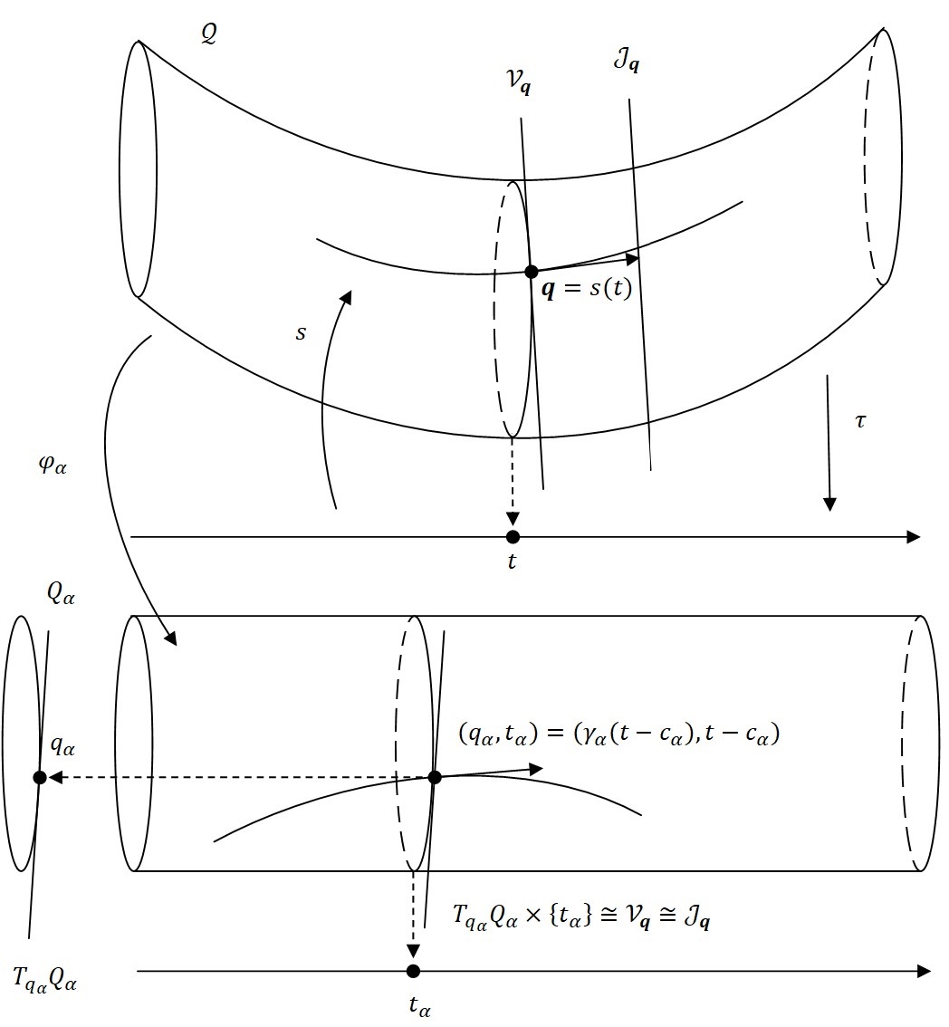
Figure 2. A section (time line) $s$ in the reference frame $\varphi_{\alpha}$.

The variational derivative of the Lagrangian $\mathbf{L}$ in the direction of vector field of virtual displacement $\underline{\eta}$ along time line $s$ is defined by

$$\delta\mathbf{L}(\underline{\eta})|_{s}:=\delta L_{\alpha}(\eta_{\alpha})|_{\gamma_{\alpha}}.$$

From Proposition 3.2, it follows that the variation derivative does not depend on the reference frame $\varphi_{\alpha}$ (see [26]). We thus have an invariant formulation of classical Lagrangian dynamics on the space-time in the form of the d’Alambert principle: a time curve $s$ is a motion of the mechanical system $(\mathcal{Q},\mathbf{L})$ if the Lagrangian derivative of $\mathbf{L}$ is equal to zero,

$$\delta\mathbf{L}(\underline{\eta})|_{s}=0,$$

for all virtual displacements $\underline{\eta}$ along $s$.

4.2. Nonholonomic systems

Let $\underline{\mathcal{A}}$ be a non-integrable distribution of rank $m+1$ of $T\mathcal{Q}$ transverse to the distribution of virtual displacements $\mathcal{V}$. We define the associated affine distribution of constraints $\mathcal{A}$ of rank $m$, a subspace of the first jet bundle $\mathcal{J}$, and the distribution of constrained virtual displacements $\mathcal{D}$ of rank $m$, a subspace of the space of virtual displacements $\mathcal{V}$, respectively by

$$\mathcal{A}=\mathcal{J}\cap\underline{\mathcal{A}},\qquad\text{and}\qquad\mathcal{D}=\mathcal{V}\cap\underline{\mathcal{A}}.$$

A time curve $s(t)$ is admissible if $\dot{s}(t)\in\mathcal{A}_{s(t)}$ for all $t\in\mathbb{R}$.

Definition 4.1.

An admissible time curve $s$ is a motion of the constrained Lagrangian system $(\mathcal{Q},\mathbf{L},\mathcal{A})$ if the variational derivative $\delta\mathbf{L}(\eta)|_{s}$ vanishes for all virtual displacements $\underline{\eta}$, sections of $\mathcal{D}$, along $s$:

$$\delta\mathbf{L}(\underline{\eta})|_{s}=0,\qquad\underline{\eta}\in\mathcal{D}.$$

In the reference frame $\varphi_{\alpha}$, the nonholonomic system $(\mathcal{Q},\mathbf{L},\mathcal{A})$ corresponds to the nonholonomic Lagrangian system $(Q_{\alpha},L_{\alpha},\mathcal{A}^{\alpha})$, where

$$\mathcal{A}^{\alpha}=\{(\mathcal{A}^{\alpha}_{t_{\alpha}},t_{\alpha}),\,|\,t_{\alpha}\in\mathbb{R}\}\subset TQ_{\alpha}\times\mathbb{R}$$

is defined from the natural identification of $\mathcal{V}$ and $\mathcal{J}$ in the reference frame $\varphi_{\alpha}$ (see (4.2),(4.3)). In other words, we have

$$\mathcal{A}^{\alpha}_{t_{\alpha}}|_{q_{\alpha}}:=\big{\{}\xi\in T_{q_{\alpha}}Q_{\alpha}\,\big{|}\,\xi+\frac{\partial}{\partial t}\in d\varphi_{\alpha}\big{(}\mathcal{A}|_{\varphi_{\alpha}^{-1}(q_{\alpha},t_{\alpha})}\big{)}\big{\}}.$$

5. The Voronec equations and time-dependent fibration

5.1. The Voronec equations

We recall the Voronec equations for nonholonomic systems [35] (in [35] Voronec derived the equations from the Lagrange-d’Alembert principle for the case of time-independent homogeneous constraints, here we adopt the notation of Bilimovic’s student Demchenko [15, 16]). Let $q=(q^{1},\dots,q^{n})$ be local coordinates of the configuration space $Q$. Consider a nonholonomic system with the Lagrangian $L=L(q,\dot{q},t)$, non-potential forces (or generalized forces) $F_{i}=F_{i}(q,\dot{q},t)$, which correspond to the coordinates $q^{i}$, $i=1,\dots,n$, and time-dependent, non-homogeneous, nonholonomic constraints of the form

(5.1) $$\dot{q}^{m+\nu}=\sum_{i=1}^{m}a_{\nu i}(q,t)\dot{q}^{i}+a_{\nu}(q,t),\qquad\nu=1,\dots,r=n-m.$$

Let $L_{c}$ be the Lagrangian $L$ after imposing the constraints (5.1). Let $K_{\nu}$ be the partial derivatives of $L$ with respect to $\dot{q}^{m+\nu}$, $\nu=1,2,\dots,r$, restricted to the constrained subspace. We assume that the constraints (5.1) are imposed after the differentiation and obtain

$$L_{c}(q^{1},\dots,q^{n},\dot{q}^{1},\dots,\dot{q}^{m},t)=L(q,\dot{q},t)|_{\dot{q}^{m+\nu}=\sum_{i=1}^{m}a_{\nu i}(q,t)\dot{q}^{i}+a_{\nu}(q,t)},$$

$$K_{\nu}(q^{1},\dots,q^{n},\dot{q}^{1},\dots,\dot{q}^{m},t)=\frac{\partial L\,\,\,}{\partial\dot{q}^{m+\nu}}(q,\dot{q},t)|_{\dot{q}^{m+\nu}=\sum_{i=1}^{m}a_{\nu i}(q,t)\dot{q}^{i}+a_{\nu}(q,t)}.$$

The Voronec equations of motion of the given noholonomic system can be represented in the following closed form:

(5.2) $$\frac{d}{dt}\frac{\partial L_{c}}{\partial\dot{q}^{i}}=\frac{\partial L_{c}}{\partial q^{i}}+F_{i}+\sum_{\nu=1}^{r}a_{\nu i}\big{(}\frac{\partial L_{c}}{\partial q^{m+\nu}}+F_{m+\nu}\big{)}+\sum_{\nu=1}^{r}K_{\nu}\big{(}\sum_{j=1}^{m}A_{ij}^{(\nu)}\dot{q}^{j}+A_{i}^{(\nu)}\big{)},$$

$i=1,\dots,m$. The components $A_{ij}^{(\nu)}$ and $A_{i}^{(\nu)}$ are functions of the time $t$ and the coordinates $q^{1},\dots,q^{n}$ given by

(5.3) $$A_{ij}^{(\nu)}=\big{(}\frac{\partial a_{\nu i}}{\partial q^{j}}+\sum_{\mu=1}^{r}a_{\mu j}\frac{\partial a_{\nu i}}{\partial q^{m+\mu}}\big{)}-\big{(}\frac{\partial a_{\nu j}}{\partial q^{i}}+\sum_{\mu=1}^{r}a_{\mu i}\frac{\partial a_{\nu j}}{\partial q^{m+\mu}}\big{)},$$

(5.4) $$A_{i}^{(\nu)}=\big{(}\frac{\partial a_{\nu i}}{\partial t}+\sum_{\mu=1}^{r}a_{\mu}\frac{\partial a_{\nu i}}{\partial q^{m+\mu}}\big{)}-\big{(}\frac{\partial a_{\nu}}{\partial q^{i}}+\sum_{\mu=1}^{r}a_{\mu i}\frac{\partial a_{\nu}}{\partial q^{m+\mu}}\big{)},\quad i,j=1,\dots,m.$$

Remark 5.1.

The equations can be rewritten more compactly using a formal expression known as the Voronec principle (see [35, 15, 16]). As Demchenko noted, the Voronec principle is similar to Hamilton’s variational principle of least action, although the system is not variational (see pages 16–19 of [15]). In the original notation: A trajectory $q(t)=(q^{1}(t),\dots,q^{n}(t))$, $t\in[t_{1},t_{2}]$, is a motion of the nonholonomic system with Lagrangian $L(q,\dot{q},t)$, generalized forces $F_{i}=F_{i}(q,\dot{q},t)$, and constraints (5.1), if

(5.5) $$\int_{t_{1}}^{t_{2}}\Big{[}\sum_{i=1}^{n}\big{(}\frac{\partial L}{\partial q^{i}}-\frac{d}{dt}\frac{\partial L}{\partial\dot{q}^{i}}+F_{i}\big{)}\delta q^{i}+\sum_{\nu=1}^{k}K_{\nu}\big{(}\frac{d}{dt}\delta q^{m+\nu}-\delta\dot{q}^{m+\nu}\big{)}\Big{]}dt=0,$$

for all virtual displacements $\delta q^{1},\dots,\delta q^{m}$ that are equal to zero for $t=t_{1}$ and $t=t_{2}$, but otherwise arbitrary. The remaining variations $\delta q^{m+1},\dots,\delta q^{n}$ are determined from the homogeneous constraints

(5.6) $$\delta q^{m+\nu}=\sum_{i=1}^{m}a_{\nu i}\delta q^{i},\qquad\nu=1,2,\dots,r.$$

Here $\frac{d}{dt}\delta q^{n+\nu}-\delta\dot{q}^{n+\nu}$ are calculated according to the relations (5.1), (5.6), using the rule

$$\frac{d}{dt}\delta q^{i}-\delta\dot{q}^{i}=0,\qquad i=1,2,\dots,m.$$

5.2. The Ehresmann connections for time-dependent nonholomic systems

Let us consider a time-dependent non-holonimic Lagrangian system $(Q,L,\mathcal{A})$. Following Bloch, Krishnaprasad, Marsden and Murray [9], we assume that the configuration space $Q$ has the structure of a fiber bundle $\pi\colon Q\to S$ over a base manifold $S$ and that the distribution of virtual displacements $\mathcal{D}_{t}$ is transversal to the fibers of $\pi$:

(5.7) $$T_{q}Q=\mathcal{D}_{t}|_{q}\oplus\mathcal{W}_{t}|_{q},\qquad\mathcal{W}_{t}|_{q}=\ker d\pi(q).$$

In other words: $\mathcal{D}_{t}$ is a time-dependent horizontal space, while $\mathcal{W}_{t}$ vertical space at $q$ the Ehresmann connection of the fibration (for the current fibration, $\mathcal{W}_{t}$ is not time-dependent, but this is relaxed in the subsection 5.4).

Next, we consider the distribution $\underline{\mathcal{A}}$ of the extended configuration space $Q\times\mathbb{R}$ as the horizontal space of the Ehresmann connection with respect to the fibration

$$\underline{\pi}\colon Q\times\mathbb{R}\to S\times\mathbb{R},\qquad\underline{\pi}(q,t)=(\pi(q),t).$$

Namely, the transversality (5.7) is equivalent to the transversality of $\underline{\mathcal{A}}$

(5.8) $$T_{(q,t)}(Q\times\mathbb{R})=\underline{\mathcal{A}}_{(q,t)}\oplus\mathcal{W}_{t}|_{q}.$$

The distribution $\underline{\mathcal{A}}$ can be regarded as the kernel of a vertical-valued one-form $\underline{\Theta}$ on $Q\times\mathbb{R}$ that satisfies

1. $\underline{\Theta}_{(q,t)}\colon T_{(q,t)}(Q\times\mathbb{R})\to\mathcal{W}_{q}$ is a linear mapping, $(q,t)\in Q\times\mathbb{R}$;

2. $\underline{\Theta}$ is a projection: $\underline{\Theta}_{(q,t)}(X_{(q,t)})=X_{(q,t)}$, for all $X_{(q,t)}\in\mathcal{W}_{q}$.

By $\underline{\xi}^{v}=\underline{\Theta}(\underline{\xi})$ and $\underline{\xi}^{h}=\underline{\xi}-\underline{\xi}^{v}$ we denote the vertical and horizontal components of a vector field on the extended configuration space $\underline{\xi}\in\mathfrak{X}(Q\times\mathbb{R})$.

The curvature $\underline{B}$ of the connection (5.8) is a vertical-valued two-form defined by

$$\underline{B}(\underline{\xi},\underline{\eta})=-\underline{\Theta}([\underline{\xi}^{h},\underline{\eta}^{h}]).$$

Let, as above, $\dim Q=n=m+r$ and $\dim S=m$. There exist local “adapted” coordinates $q=(q^{1},\dots,q^{n})$ on $Q$ such that $(q^{1},\dots,q^{m})$ are the local coordinates on $S$, the projections $\pi\colon Q\to S$ and $\underline{\pi}\colon Q\times\mathbb{R}\to S\times\mathbb{R}$ have the form

$$\pi\colon(q^{1},\dots,q^{m},q^{m+1},\dots,q^{n})\longmapsto(q^{1},\dots,q^{m}),$$

$$\underline{\pi}\colon(q^{1},\dots,q^{m},q^{m+1},\dots,q^{n},t)\longmapsto(q^{1},\dots,q^{m},t)$$

and the constraints defining $\mathcal{A}_{t}$ are given by (5.1). Then we have locally

$$\underline{\Theta}=\sum_{\nu=1}^{r}\omega^{\nu}\frac{\partial}{\partial q^{m+\nu}},\quad\omega^{\nu}=dq^{n+\nu}-\sum_{i=1}^{m}a_{\nu i}dq^{i}-a_{\nu}dt,$$

$$X^{h}=\big{(}\sum_{l=1}^{n}X^{l}\frac{\partial}{\partial q^{l}}+X_{t}\frac{\partial}{\partial t}\big{)}^{h}=\sum_{i=1}^{m}X^{i}\frac{\partial}{\partial q^{i}}+X_{t}\frac{\partial}{\partial t}+\sum_{\nu=1}^{r}\big{(}\sum_{i=1}^{m}a_{\nu i}X^{i}+a_{\nu}X_{t}\big{)}\frac{\partial}{\partial q^{m+\nu}},$$

$$X^{v}=\big{(}\sum_{l=1}^{n}X^{l}\frac{\partial}{\partial q^{l}}\big{)}^{v}=\sum_{\nu=1}^{r}\big{(}X^{m+\nu}-\sum_{i=1}^{m}a_{\nu i}X^{i}-a_{\nu}X_{t}\big{)}\frac{\partial}{\partial q^{m+\nu}},$$

$$\underline{B}(\frac{\partial}{\partial q^{i}},\frac{\partial}{\partial q^{j}})=\sum_{\nu=1}^{r}B^{\nu}_{ij}\frac{\partial}{\partial q^{m+\nu}},$$

$$\underline{B}(\frac{\partial}{\partial q^{i}},\frac{\partial}{\partial t})=\sum_{\nu=1}^{r}B^{\nu}_{i,t}\frac{\partial}{\partial q^{m+\nu}},\quad\underline{B}(\frac{\partial}{\partial t},\frac{\partial}{\partial q^{i}})=\sum_{\nu=1}^{r}B^{\nu}_{t,i}\frac{\partial}{\partial q^{m+\nu}}.$$

Here $B_{ij}^{\nu}(q,t)=A^{(\nu)}_{ij}(q,t)$, $B_{i,t}^{\nu}(q,t)=A^{(\nu)}_{i}(q,t)$, $B_{t,i}^{\nu}(q,t)=-A^{(\nu)}_{i}(q,t)$, where $A^{(\nu)}_{ij}(q,t)$, $A^{\nu}_{i}(q,t)$ are derived from the Voronec equations (5.3) (5.4), $i,j=1,\dots,m$, while the other components of the curvature are zero. To the author’s knowledge, the above curvature interpretation of the Voronec coefficients is (5.3) (5.4) for time-dependent non-homogeneous constraints was first given by Bakša [4].

Example 5.1.

In Example 2.1 we have $m=1$, $n=2$, $(q^{1},q^{2})=(y,x)$ and

$$B_{1,t}=\frac{\partial a}{\partial t}-\frac{\partial b}{\partial y}+b\frac{\partial a}{\partial x}-a\frac{\partial b}{\partial x},\qquad B_{t,1}=-B_{1,t}.$$

The distribution $\underline{\mathcal{A}}$ is therefore a contact if and only if the curvature $\underline{B}$ is different from zero.

Remark 5.2.

Similarly, $\mathcal{D}_{t}$ can be seen as the kernel of a time-dependent vector-valued one form $\Theta_{t}$ on $Q$ with properties (i) and (ii) for the fibration $\pi$. Locally, $\Theta_{t}$ is given by the same equation as $\underline{\Theta}$, where $\omega^{\nu}$ is replaced by $\omega^{\nu}_{t}=dq^{n+\nu}-\sum_{i=1}^{m}a_{\nu i}dq^{i}$ (see e.g. [9] for the time-independent case). Let $B_{t}$ be the corresponding time-dependent curvature

$${B_{t}}({\xi},{\eta})=-{\Theta_{t}}([{\xi}^{h},{\eta}^{h}]),\qquad\xi,\eta\in\mathfrak{X}(Q).$$

Since $\mathcal{D}_{t}$ is tangent to the foliation $\{(q,t)\in Q\times\mathbb{R}\,|\,t=const\}$ and $\mathcal{D}_{t}|_{q}\subset\underline{\mathcal{A}}_{(q,t)}$, from the definition of the curvature we have

$$B_{t}|_{\mathcal{D}_{t}|_{q}\times\mathcal{D}_{t}|_{q}}=\underline{B}|_{\mathcal{D}_{t}|_{q}\times\mathcal{D}_{t}|_{q}},\quad B_{t}(\mathcal{W}_{t}|_{q},T_{q}Q)\equiv 0,\quad\underline{B}(\mathcal{W}_{t}|_{q},T_{(q,t)}Q\times\mathbb{R})\equiv 0.$$

The components of the curvature $B_{t}$ of the time-dependent connection $D_{t}$ are the same as the corresponding components of the curvature $\underline{B}$

$$B_{t}(\frac{\partial}{\partial q^{i}},\frac{\partial}{\partial q^{j}})=\sum_{\nu=1}^{r}B^{\nu}_{ij}\frac{\partial}{\partial q^{m+\nu}},\qquad i,j=1,\dots,n.$$

Remark 5.3.

Note that, even if the constraint are homogeneous $\mathcal{A}_{t}=\mathcal{D}_{t}$, the components of the curvature $B_{t,i}$ are different from zero in the time-dependent case.

Let $\theta_{t}$ be a vertical-valued vector field given by

$$\theta_{t}=\big{(}\frac{\partial}{\partial t}\big{)}^{v}=\underline{\Theta}\big{(}\frac{\partial}{\partial t}\big{)}.$$

Lemma 5.1.

The affine subspace $\mathcal{A}_{t}|_{q}\subset T_{q}Q$ is the image of the tangent space $T_{q}Q$ under the composition of affine and linear mappings

$$\mathrm{pr}_{t}\colon\eta\in T_{q}Q\longmapsto\big{(}\eta+\frac{\partial}{\partial t}\big{)}^{h}-\frac{\partial}{\partial t}=\eta^{h}+\theta_{t}\in\mathcal{A}_{t}|_{q}.$$

Note that $\mathrm{pr}_{t}$ is the identity mapping restricted to ${\mathcal{A}_{t}|_{q}}$. In other words, $\mathrm{pr}_{t}$ is an affine projection. In particular, we have

$$\mathcal{A}_{t}=\mathcal{D}_{t}+\theta_{t}.$$

Let $L_{c}\colon TQ\times\mathbb{R}\to\mathbb{R}$ be the constrained Lagrangian defined by

$$L_{c}(q,\dot{q},t):=L(q,\mathrm{pr}_{t}(\dot{q}),t)=L(q,\dot{q}^{h}+\theta_{t},t),$$

The Voronec principle (5.5) can be expressed in invariant form as follows.

Theorem 5.1.

An admissible curve $\gamma$ is a motion of the constrained Lagrangian system $(Q,L,\mathbf{F},\mathcal{A})$ if and only if

(5.9) $$\delta L_{c}(\eta)|_{\gamma}+\mathbf{F}(\eta)|_{\gamma}=\mathbb{F}L(q,\mathrm{pr}_{t}(\dot{q}),t)(\underline{B}(\dot{q}+\frac{\partial}{\partial t},\eta))|_{\gamma}$$

for all virtual displacements $\eta=\sum_{s=1}^{n}\eta^{s}\frac{\partial}{\partial q_{s}}\in\mathcal{D}_{t}|_{\gamma(t)}$ along $\gamma$.

Here $\delta L_{c}(\eta)$ is the variational derivative of $L_{c}$ along the virtual displacements $\eta$ and:

$$\mathbb{F}L(q,\mathrm{pr}_{t}(\dot{q}),t) \big{(}\underline{B}\big{(}\dot{q}+\frac{\partial}{\partial t},\eta\big{)}\big{)}|_{\gamma}=\mathbb{F}L(q,\mathrm{pr}_{t}(\dot{q}),t)\big{(}B_{t}(\dot{q},\eta)+\underline{B}\big{(}\frac{\partial}{\partial t},\eta\big{)}\big{)}|_{\gamma}$$

$$= \sum_{\nu=1}^{m}\frac{\partial L}{\partial\dot{q}_{m+\nu}}|_{\dot{q}^{m+\nu}=\sum_{i=1}^{m}a_{\nu i}(q,t)\dot{q}^{i}+a_{\nu}(q,t)}\big{(}B^{\nu}_{t}(\dot{q},\eta)+\sum_{s=1}^{n}B_{t,s}^{\nu}\eta^{s}\big{)}|_{\gamma}.$$

Note that the restrictions of the constrained Lagrangian $L_{c}$ and the Lagrangian $L$ on the affine distribution coincide:

$$L_{c}|_{\mathcal{A}_{t}}=L|_{\mathcal{A}_{t}}.$$

5.3. Natural mechanical systems

Let us consider the Lagrangian

$$L(q,\dot{q},t)=\frac{1}{2}K_{t}(\dot{q},\dot{q})+\Delta_{t}(\dot{q})-V(q,t)$$

of a natural mechanical system. Then the constrained Lagrangian reads

$$L_{c}(q,\dot{q},t)=\frac{1}{2}K_{t}(\dot{q}^{h},\dot{q}^{h})+\big{(}K_{t}(\theta_{t},\dot{q}^{h})+\Delta_{t}(\dot{q}^{h})\big{)}+\big{(}\frac{1}{2}K_{t}(\theta_{t},\theta_{t})+\Delta_{t}(\theta_{t})-V(q,t)\big{)}$$

Since the fiber derivative is given by (3.2), the right-hand side of the system (5.9) is

$$\mathbb{F}L(q, \mathrm{pr}_{t}(\dot{q}),t)(\underline{B}(\dot{q}+\frac{\partial}{\partial t},\eta))=K_{t}(\dot{q}^{h},B_{t}(\dot{q},\eta))+K_{t}(\theta_{t},B_{t}(\dot{q},\eta))$$

$$+\Delta_{t}(B_{t}(\dot{q},\eta))+K_{t}(\dot{q}^{h},\underline{B}\big{(}\frac{\partial}{\partial t},\eta\big{)})+K_{t}(\theta_{t},\underline{B}\big{(}\frac{\partial}{\partial t},\eta\big{)})+\Delta_{t}(\underline{B}\big{(}\frac{\partial}{\partial t},\eta\big{)}).$$

5.4. The Ehresmann connection in the moving frame

Next, we consider the moving frame $g_{t}\colon M\to Q$. As a result, the moving configuration space $M$ has the structure of a time-dependent fiber bundle $\Pi_{t}\colon M\to S$ defined by

$$\Pi_{t}(x):=\pi(g_{t}(x)),$$

The distribution of the virtual displacements $\mathbf{D}_{t}$ is transverse to the fibers of $\Pi_{t}$:

$$T_{x}M=\mathbf{D}_{t}|_{x}\oplus\mathbf{W}_{t}|_{x},\qquad\mathbf{W}_{t}|_{x}=\ker d\Pi_{t}(x)=dg_{t}^{-1}(\mathcal{W}_{t}|_{q}),$$

and $\mathbf{D}_{t}$ and $\mathbf{W}_{t}$ are horizontal space and vertical space at $x$ of the Ehresmann connection of the time-dependent fibration $\Pi_{t}$.

As above, we consider the distribution $\underline{\mathbf{A}}$ of the extended configuration space $M\times\mathbb{R}$ as the horizontal space of the Ehresmann connection

(5.10) $$T_{(x,t)}(M\times\mathbb{R})=\underline{\mathbf{A}}_{(x,t)}\oplus\mathbf{W}_{t}|_{x}.$$

related to the fibration

$$\underline{\Pi}\colon M\times\mathbb{R}\to N\times\mathbb{R},\qquad\underline{\Pi}(x,t)=(\Pi_{t}(x),t).$$

Again, we define the curvature $\underline{\mathbf{B}}$ of the connection (5.10), the projection

$$\mathbf{pr}_{t}\colon\xi\in T_{x}M\longmapsto\big{(}\xi+\frac{\partial}{\partial t}\big{)}^{h}-\frac{\partial}{\partial t}\in\mathbf{A}_{t}|_{x},$$

and the constrained Lagrangian $l_{c}$:

$$l_{c}(x,\dot{x},t):=l(x,\mathbf{pr}_{t}(\dot{x}),t).$$

Note that, equivalently, the constrained Lagrangian $l_{c}$ can be defined from the constrained Lagrangian $L_{c}$ in the fixed frame:

$$l_{c}(x,\dot{x},t):=L_{c}(q,\dot{q},t)|_{q=g_{t}(x),\dot{q}=dg_{t}(\dot{x})+\omega_{t}(g_{t}(x))}.$$

This means that we have

Lemma 5.2.

The following diagram is commutative

where the horizontal lines denote the mapping $\xi\mapsto dg_{t}(\xi)+\omega_{t}|_{q}$, $q=dg_{t}(x)$.

As a result we have.

Proposition 5.1.

An admissible curve $\Gamma(t)$ is a motion of the constrained Lagrangian system in the moving frame $(M,l,\mathbf{f},\mathbf{A})$ if

$$\delta l_{c}(\xi)|_{\Gamma}+\mathbf{f}(\xi)|_{\Gamma}=\mathbb{F}l(x,\dot{x},t)(\underline{\mathbf{B}}(\dot{x}+\frac{\partial}{\partial t},\xi))|_{\Gamma}$$

for all virtual displacements $\xi=\sum_{s=1}^{n}\xi^{s}\frac{\partial}{\partial x_{s}}\in\mathbf{D}_{t}|_{\Gamma(t)}$ along $\Gamma$.

6. Time-dependent Chaplygin systems

6.1. Definitions

In addition to the assumptions from section 5, we now assume that the time-dependent fibration $\pi_{t}:Q\to S$ is determined by a time-dependent free action of an $r$–dimensional Lie group $G$ on $Q$ and the affine constraint space $\mathcal{A}_{t}$ and the distribution of virtual displacements $\mathcal{D}_{t}$ are $G$–invariant Then the $G$–orbit $\mathcal{O}_{t}(q)$ through a point $q$ is the fiber $\pi_{t}(\pi_{t}(q))$, $t\in\mathbb{R}$ (see Fig. 3). The decomposition

$$T_{q}Q=\mathcal{D}_{t}|_{q}\oplus\mathcal{W}_{t}|_{q},\qquad\mathcal{W}_{t}|_{q}=\ker d\pi_{t}(q)=T_{q}(\mathcal{O}_{t}(q)),$$

is $G$–invariant and $\mathcal{D}_{t}$ is a principal connection of a time-dependent principal bundle $G\longrightarrow Q\longrightarrow S=Q/G$ (here a time $t$ is fixed). On the other hand, the decomposition

(6.1) $$T_{(q,t)}(Q\times\mathbb{R})=\underline{\mathcal{A}}_{(q,t)}\oplus\mathcal{W}_{t}|_{q},$$

is also $G$–invariant and $\underline{\mathcal{A}}$ is a principal connection of the principal bundle

$$\lx@xy@svg{\hbox{\raise 0.0pt\hbox{\kern 6.93124pt\hbox{\ignorespaces\ignorespaces\ignorespaces\hbox{\vtop{\kern 0.0pt\offinterlineskip\halign{\entry@#!@&&\entry@@#!@\cr&\\&\crcr}}}\ignorespaces{\hbox{\kern-6.93124pt\raise 0.0pt\hbox{\hbox{\kern 0.0pt\raise 0.0pt\hbox{\hbox{\kern 3.0pt\raise 0.0pt\hbox{$\textstyle{G\ignorespaces\ignorespaces\ignorespaces\ignorespaces}$}}}}}}}\ignorespaces\ignorespaces\ignorespaces\ignorespaces{}{\hbox{\lx@xy@droprule}}\ignorespaces{\hbox{\kern 34.93124pt\raise 0.0pt\hbox{\hbox{\kern 0.0pt\raise 0.0pt\hbox{\lx@xy@tip{1}\lx@xy@tip{-1}}}}}}{\hbox{\lx@xy@droprule}}{\hbox{\lx@xy@droprule}}{\hbox{\kern 34.93124pt\raise 0.0pt\hbox{\hbox{\kern 0.0pt\raise 0.0pt\hbox{\hbox{\kern 3.0pt\raise 0.0pt\hbox{$\textstyle{Q\times\mathbb{R}\ignorespaces\ignorespaces\ignorespaces\ignorespaces}$}}}}}}}\ignorespaces\ignorespaces\ignorespaces\ignorespaces{}{\hbox{\lx@xy@droprule}}\ignorespaces\ignorespaces\ignorespaces{\hbox{\kern 50.56456pt\raise-21.11108pt\hbox{{}\hbox{\kern 0.0pt\raise 0.0pt\hbox{\hbox{\kern 3.0pt\hbox{\hbox{\kern 0.0pt\raise-2.83888pt\hbox{$\scriptstyle{\underline{\pi}}$}}}\kern 3.0pt}}}}}}\ignorespaces{\hbox{\kern 50.56456pt\raise-32.38887pt\hbox{\hbox{\kern 0.0pt\raise 0.0pt\hbox{\lx@xy@tip{1}\lx@xy@tip{-1}}}}}}{\hbox{\lx@xy@droprule}}{\hbox{\lx@xy@droprule}}{\hbox{\kern-3.0pt\raise-42.22218pt\hbox{\hbox{\kern 0.0pt\raise 0.0pt\hbox{\hbox{\kern 3.0pt\raise 0.0pt\hbox{$\textstyle{}$}}}}}}}{\hbox{\kern 35.52986pt\raise-42.22218pt\hbox{\hbox{\kern 0.0pt\raise 0.0pt\hbox{\hbox{\kern 3.0pt\raise 0.0pt\hbox{$\textstyle{S\times\mathbb{R}}$}}}}}}}\ignorespaces}}}}\ignorespaces,\qquad\underline{\pi}(q,t)=(\pi_{t}(q),t). \textstyle{G\ignorespaces\ignorespaces\ignorespaces\ignorespaces} \textstyle{Q\times\mathbb{R}\ignorespaces\ignorespaces\ignorespaces\ignorespaces} \scriptstyle{\underline{\pi}} \textstyle{S\times\mathbb{R}} \textstyle{G\ignorespaces\ignorespaces\ignorespaces\ignorespaces} \textstyle{Q\times\mathbb{R}\ignorespaces\ignorespaces\ignorespaces\ignorespaces} \scriptstyle{\underline{\pi}} \textstyle{S\times\mathbb{R}}$$

Let, $y=\pi_{t}(q)$. For vectors $\xi\in T_{y}S$, $\underline{\xi}\in T_{(y,t)}(S\times\mathbb{R})$, the horizontal lifts $\mathbb{H}^{q}_{t}({\xi})\in{\mathcal{D}}_{t}|_{q}$ and $\mathbb{H}^{(q,t)}(\underline{\xi})\in\underline{\mathcal{A}}_{(q,t)}$ are the unique vectors, such that

$$d{\pi_{t}}(\mathbb{H}^{q}_{t}(\xi))={\xi},\qquad d\underline{\pi}(\mathbb{H}^{(q,t)}(\underline{\xi}))=\underline{\xi}.$$

In addition, we define the affine horizontal lift of $\xi\in T_{y}S$ by (see Fig. 3)

$$\mathbb{A}^{q}_{t}(\xi)=\mathrm{pr}_{t}\mathbb{H}^{q}_{t}\big{(}\xi\big{)}=\mathbb{H}^{q}_{t}\big{(}\xi\big{)}+\theta_{t}|_{q}\in\mathcal{A}_{t}|_{q}.$$

Figure 3. The horizontal and affine horizontal lift of a vector $\xi\in T_{y}S$.

Note that the Ehresmann curvature $\underline{B}$ of the principal connection (6.1) via the identification $\mathcal{W}_{t}\cong\mathfrak{g}$ can be understood as a $\mathfrak{g}$-valued 2-form on $Q$.

By analogy with time-independent $G$–Chaplygin systems [29, 9] and $G$–Chaplygin systems with gyroscopic forces [17] we define.

Definition 6.1.

Let $L$ be a time-dependent $G$–invariant Lagrangian and let $\mathbf{F}$ be a field of time-dependent $G$–invariant non-potential forces on $Q$. The reduced Lagrangian $L_{red}(y,\dot{y},t)$ and the reduced field of non-potential forces $\mathbf{F}(y,\dot{y},t)$ on $S$ are defined by

$$L(y,\dot{y},t):=L(q,\mathbb{A}^{q}_{t}(\dot{y}),t),\quad\mathbf{F}_{red}(y,\dot{y},t)(\xi):=\mathbf{F}(\mathbb{A}^{q}_{t}(\dot{y}),t)(\mathbb{H}_{t}^{q}(\xi)),\quad\xi\in T_{y}S,$$

where $q$ is any element of the fiber $\pi_{t}^{-1}(y)$. The JK term is defined by

$${\mathbf{JK}}(y,\dot{y},t)(\xi):=\mathbb{F}L(q,\mathbb{A}_{t}^{q}(\dot{y}),t)(\underline{B}\big{(}\mathbb{H}^{(q,t)}\big{(}\dot{y}+\frac{\partial}{\partial t}\big{)},\mathbb{H}^{q}_{t}(\xi))\big{)}$$

In local coordinates $(y^{1},\dots,y^{m})$ on $S=Q/G$ we have

$${\mathbf{JK}}=\sum_{i=1}^{m}{\mathbf{JK}}_{i}(y,\dot{y},t)dy^{i},\qquad\mathbf{F}_{red}=\sum_{i=1}^{m}F_{red,i}(y,\dot{y},t)dy^{i}.$$

The equations (5.9) are $G$–invariant and they reduce to $TS$:

(6.2) $$\delta L_{red}(\xi)+\mathbf{F}_{red}(\xi)=\mathbf{JK}(y,\dot{y},t)(\xi)\qquad\text{for all}\quad\xi\in T_{y}S,$$

or, in local coordinates,

$$\frac{d}{dt}\frac{\partial l}{\partial\dot{y}_{i}}=\frac{\partial L}{\partial y_{i}}+F_{red,i}(y,\dot{y},t)-\mathbf{JK}_{i}(y,\dot{y},t),\qquad i=1,\dots,m.$$

Definition 6.2.

We refer to $(Q,L,\mathbf{F},\mathcal{A},G)$ as a time-dependent $G$–Chaplygin system, and to $(S,L_{red},\mathbf{F}_{red},{\mathbf{JK}})$ as a reduced time-dependent $G$–Chaplygin system.

We summarize the above consideration in the following statement.

Theorem 6.1.

A solution $\gamma(t)$ of the time-dependent $G$–Chaplygin system $(Q,L,\mathbf{F},\mathcal{A},G)$ projects to a solution $\Gamma(t)=\pi_{t}(\gamma(t))$ of the reduced time-dependent $G$–Chaplygin system $(S,L_{red},\mathbf{F}_{red},{\mathbf{JK}})$. Conversely, let $\Gamma(t)$ be a solution of the reduced system (6.2) with the initial conditions $\Gamma(0)=y_{0}$, $\dot{\Gamma}(0)=Y_{0}\in T_{y_{0}}S$ and let $q_{0}\in\pi^{-1}(y_{0})$. Then the affine horizontal lift $\gamma(t)$ of $\Gamma(t)$ through $q_{0}$ is the solution of the original system with the initial conditions $\gamma(0)=y_{0}$, $\dot{\gamma}(0)=\mathbb{A}_{t}^{q_{0}}(Y_{0})\in\mathcal{A}_{t}|_{q_{0}}$.

Remark 6.1.

In the case the group $G$ is Abelian, we do not need an invariant formulation of the Voronec equations, which we obtain in Theorem 5.1 and Proposition 5.1. One can perform the reduction procedure directly by using the classical Voronec equations (5.2), where the Lagrangian $L$ and the constraints (5.1) do not depend on $q^{m+\nu}$ and the action of the group $G$ is simply given by the translations in the coordinates $q^{m+\nu}$, $\nu=1,\dots,n-m$ (classical Chaplygin systems [14]).

6.2. Natural mechanical systems

The above construction can be related to the standard construction for time-independent natural mechanical systems. In the case that we have a natural mechanical system with the Lagrangian

$$L(q,\dot{q},t)=\frac{1}{2}K_{t}(\dot{q},\dot{q})+\Delta_{t}(\dot{q})-V(q,t),$$

we define

Definition 6.3.

Let $K_{t}$, $\Delta_{t}$, and $V(q,t)$ be a $G$–invariant metric, 1-form, and a potential on $Q$. The reduced metric $K_{red,t}$, the reduced 1-form $\Delta_{red,t}$ and the reduced potential $V_{red}$ on $S$ are defined by:

$$K_{red,t}(\xi_{1},\xi_{2})|_{y}=K_{t}(\mathbb{H}^{q}_{t}(\xi_{1}),\mathbb{H}^{q}_{t}(\xi_{2}))|_{q},$$

$$\Delta_{red,t}(\xi)=K_{t}(\theta_{t}|_{q},\mathbb{H}^{q}_{t}(\xi))+\Delta_{t}(\mathbb{H}^{q}_{t}(\xi))\big{)},$$

$$V_{red}(y,t)=V(q,t)-\frac{1}{2}K_{t}(\theta_{t}|_{q},\theta_{t}|_{q})-\Delta_{t}(\theta_{t}|_{q}),\qquad y=\pi(q).$$

The reduced Lagrangian is then

$$L_{red}(y,\dot{y},t)=\frac{1}{2}K_{red,t}(\dot{y},\dot{y}))+\Delta_{red,t}(\dot{y})-V_{red}(y,t).$$

On the other hand, the JK term has the form

$${\mathbf{JK}}(y,\dot{y},t)(\xi)={\mathbf{JK}}^{2}(y,\dot{y},t)(\xi)+{\mathbf{JK}}^{1}(y,\dot{y},t)(\xi)+{\mathbf{JK}}^{0}(y,\dot{y},t)(\xi),$$

where

$${\mathbf{JK}}^{2}(y,\dot{y},t)(\xi)= K_{t}\big{(}\mathbb{H}^{q}_{t}(\dot{y}),B_{t}(\mathbb{H}^{q}_{t}(\dot{y}),\mathbb{H}^{q}_{t}(\xi))\big{)}$$

$${\mathbf{JK}}^{1}(y,\dot{y},t)(\xi)= K_{t}\big{(}\theta_{t}|_{q},B_{t}(\mathbb{H}^{q}_{t}(\dot{y}),\mathbb{H}^{q}_{t}(\xi)\big{)}$$

$$+\Delta_{t}\big{(}B_{t}(\mathbb{H}^{q}_{t}(\dot{y}),\mathbb{H}^{q}_{t}(\xi)\big{)}+K_{t}\big{(}\mathbb{H}^{q}_{t}(\dot{y}),\underline{B}\big{(}\frac{\partial}{\partial t},\mathbb{H}^{q}_{t}(\xi)\big{)}\big{)}$$

$${\mathbf{JK}}^{0}(y,\dot{y},t)(\xi)= K_{t}\big{(}\theta_{t},\underline{B}\big{(}\frac{\partial}{\partial t},\mathbb{H}^{q}_{t}(\xi)\big{)}\big{)}+\Delta_{t}\big{(}\underline{B}\big{(}\frac{\partial}{\partial t},\mathbb{H}^{q}_{t}(\xi)\big{)}\big{)}.$$

Here the first term is quadratic in velocities and is a time-dependent version of the well-studied $(0,3)$-tensor in nonholonomic mechanics

$$\Sigma_{t}(\xi_{1},\xi_{2},\xi_{3})|_{y}=K_{t}\big{(}\mathbb{H}^{q}_{t}(\xi_{1}),B_{t}(\mathbb{H}^{q}_{t}(\xi_{2}),\mathbb{H}^{q}_{t}(\xi_{3}))\big{)}|_{q},\qquad q\in\pi^{-1}(y).$$

The $(0,3)$-tensor $\Sigma_{t}$ is skew-symmetric with respect to the second and third argument, and

$${\mathbf{JK}}^{2}(y,\dot{y},t)(\xi)=\Sigma_{t}(\dot{y},\dot{y},\xi).$$

After [14], one of the central problems in the study of natural-mechanical Chaplygin systems is the Chaplygin-Hamiltonization using the time reparamitrazition (see e.g [10, 13, 21, 22, 23, 17] and references therein). In [10] and [17] the problem is extended to the case of an addition of a gyroscopic term $\mathbf{F}_{red}$.

In the time-dependent case, the simplest situation is when we use a distinguish reference frame in which $\theta_{t}\equiv 0$ and the linear term in the Lagrangian also vanishes $\Delta_{t}\equiv 0$. Then the JK term of zero degree ${\mathbf{JK}}^{0}$ vanishes and the linear JK term simplifies to

$${\mathbf{JK}}^{1}(y,\dot{y},t)(\xi)=K_{t}(\mathbb{H}^{q}_{t}(\dot{y}),\underline{B}\big{(}\frac{\partial}{\partial t},\mathbb{H}^{q}_{t}(\xi)\big{)})\\$$

Probably, the study of the problem of Hamiltonization of the time-dependent Chaplygin system should be started with these assumptions. The following is a first step in this direction.

6.3. Rolling of a disc over a circle of variable radius - a nonholonomic system with one-dimensional constraint distribution

An illustrative example is the rolling without sliding of a disc with radius $r$, mass $m$ and centre $S$ over a vertical circle with variable radius $R(t)$ and centre at point $O$. The configuration space is $\mathbb{R}^{2}\{s_{1},s_{2}\}\times S^{1}\{\psi\}$. The coordinates $(s_{1},s_{2})$ determine the position of the centre of the disc $S$, $\overrightarrow{OS}=s_{1}\vec{e}_{1}+s_{2}\vec{e}_{2}$, and the angle $\psi$ is the angle of rotation $B(\psi)$ between the fixed reference frame $[O,\vec{e}_{1},\vec{e}_{2}]$ and the reference frame $[S,\vec{E}_{1},\vec{E}_{2}]$ attached to the disc (see Fig. 4):

$$\vec{E}_{1}=\cos\psi\vec{e}_{1}+\sin\psi\vec{e}_{2},\qquad\vec{E}_{2}=-\sin\psi\vec{e}_{1}+\cos\psi\vec{e}_{2}.$$

In other words, the coordinates of a point $X$ in two reference frames are related by the Euclidean motion

(6.3) $$\begin{pmatrix}q_{1}\\ q_{2}\end{pmatrix}=\begin{pmatrix}\cos\psi&-\sin\psi\\ \sin\psi&\cos\psi\end{pmatrix}\begin{pmatrix}x_{1}\\ x_{2}\end{pmatrix}+\begin{pmatrix}s_{1}\\ s_{2}\end{pmatrix},$$

$\overrightarrow{OX}=q_{1}\vec{e}_{1}+q_{2}\vec{e}_{2}$, $\overrightarrow{SX}=x_{1}\vec{E}_{1}+x_{2}\vec{E}_{2}$.

Figure 4. Rolling of a disc of radius $r$, center $S$ and mass center $S$ over a vertical circle of variable radius $R(t)$ and center $O$.

Let us consider a point $X(x_{1},x_{2})$ that is fixed in the frame $[S,\vec{E}_{1},\vec{E}_{2}]$. From (6.3) it follows that its velocity in the frame $[O,\vec{e}_{1},\vec{e}_{2}]$ is

$$\begin{pmatrix}v_{1}\\ v_{2}\end{pmatrix}= \frac{d}{dt}\big{(}\begin{pmatrix}\cos\psi&-\sin\psi\\ \sin\psi&\cos\psi\end{pmatrix}\begin{pmatrix}x_{1}\\ x_{2}\end{pmatrix}+\begin{pmatrix}s_{1}\\ s_{2}\end{pmatrix}\big{)}=\dot{\psi}\begin{pmatrix}-\sin\psi&-\cos\psi\\ \cos\psi&-\sin\psi\end{pmatrix}\begin{pmatrix}x_{1}\\ x_{2}\end{pmatrix}+\begin{pmatrix}\dot{s}_{1}\\ \dot{s}_{2}\end{pmatrix}$$

$$= \dot{\psi}\begin{pmatrix}-\sin\psi&-\cos\psi\\ \cos\psi&-\sin\psi\end{pmatrix}\begin{pmatrix}\cos\psi&-\sin\psi\\ \sin\psi&\cos\psi\end{pmatrix}^{-1}\begin{pmatrix}X_{1}\\ X_{2}\end{pmatrix}+\begin{pmatrix}\dot{s}_{1}\\ \dot{s}_{2}\end{pmatrix}$$

$$= \begin{pmatrix}0&-\dot{\psi}\\ \dot{\psi}&0\end{pmatrix}\begin{pmatrix}X_{1}\\ X_{2}\end{pmatrix}+\begin{pmatrix}\dot{s}_{1}\\ \dot{s}_{2}\end{pmatrix},\qquad\text{where}\qquad\overrightarrow{SX}=X_{1}\vec{e}_{1}+X_{2}\vec{e}_{2},$$

that is,

(6.4) $$(v_{1},v_{2})=\dot{\psi}(-X_{2},X_{1})+(\dot{s}_{1},\dot{s}_{2}).$$

We have a holonomic constraint

$$f(s,t)=s_{1}^{2}+s_{2}^{2}-(R(t)+r)^{2}=0,$$

and instead of the coordinates $(s_{1},s_{2})$ we can use the angular coordinate $\varphi$, so that

$$(s_{1},s_{2})=((R+r)\cos\varphi,(R+r)\sin\varphi).$$

For the configuration space $Q$ we can therefore take a torus $Q=S^{1}\times S^{1}\{\varphi,\psi\}$.

Let $A$ be a point of contact. The non-sliding condition at $A$ means that the velocity of the point $A$, considered as a point of the circle with coordinates $(R\cos\varphi,R\sin\varphi)$ in the frame $[O,\vec{e}_{1},\vec{e}_{2}]$,

(6.5) $$(v_{A1},v_{A2})=\dot{R}\cdot(\cos\varphi,\sin\varphi),$$

coincides to the velocity of the point $A$, which is considered as the point of the disc with the coordinates $(x_{A1},x_{A2})$ in the frame $[S,\vec{E}_{1},\vec{E}_{2}]$. From (6.4) and (6.5) we get

$$\dot{R}(\cos\varphi,\sin\varphi)=\dot{\psi}(r\sin\varphi,-r\cos\varphi)+\dot{R}(\cos\varphi,\sin\varphi)+(R+r)\dot{\varphi}(-\sin\varphi,\cos\varphi),$$

Therefore, we obtain a homogeneous constraint

(6.6) $$\mathcal{A}_{t}=\mathcal{D}_{t}\colon\qquad r\dot{\psi}-(R+r)\dot{\varphi}=0.$$

If the constraint (6.6) is stationary, $\dot{R}\equiv 0$, then it is integrable. For a given initial condition, the system is a 1-dimensional time-independent holonomic system and therefore completely integrable. Otherwise, we have a nonholonomic system (see Example 2.1) with a constraint defining the Ehresmann connections for the fibrations $\pi\colon Q\to S^{1}$, $\pi(\varphi,\psi)=\varphi$ and $\pi(\varphi,\psi)=\psi$. We will use the first variant in the following.

Without loss of generality, we assume that the centre of mass $C$ of the disc has the coordinates $(x_{C1},x_{C2})=(c,0)$. Then

$$(X_{C1},X_{C2})=(c\cos\psi,c\sin\psi),\quad(q_{C1},q_{C2})=((R+r)\cos\varphi,(R+r)\sin\varphi)+(c\cos\psi,c\sin\psi),$$

and the gravitational potential energy of the system is

$$v_{g}(\varphi,\psi,t)=mgq_{C2}=mg\big{(}(R(t)+r)\sin\varphi+c\sin\psi\big{)},$$

while the kinetic energy is given by

$$T(\varphi,\psi,\dot{\varphi},\dot{\psi},t)= \frac{1}{2}m\big{(}\dot{s}_{1}^{2}+\dot{s}_{2}^{2}\big{)}+\frac{1}{2}I\dot{\psi}^{2}+m\dot{\psi}(X_{C1}\dot{s}_{2}-X_{C2}\dot{s}_{1})$$

$$= \frac{1}{2}m\big{(}(R+r)^{2}\dot{\varphi}^{2}+\dot{R}^{2}\big{)}+\frac{1}{2}I\dot{\psi}^{2}$$

$$+cm\dot{\psi}\big{(}\dot{R}(\cos\psi\sin\varphi-\sin\psi\cos\varphi)+\dot{\varphi}(R+r)(\cos\psi\cos\varphi+\sin\psi\sin\varphi)\big{)},$$

where $I$ is the moment of inertia of the disc with respect to the point $S$.

As a result, we obtain a time-dependent natural mechanical system on a torus with the Lagrangian $L=\frac{1}{2}K_{t}+\Delta_{t}-V$, where

$$K_{t}\big{(}(\dot{\varphi},\dot{\psi}),(\dot{\varphi},\dot{\psi})\big{)}=m(R+r)^{2}\dot{\varphi}^{2}+I\dot{\psi}^{2}+2cm\dot{\psi}\dot{\varphi}(R+r)\cos(\varphi-\psi),$$

$$\Delta_{t}\big{(}(\dot{\varphi},\dot{\psi})\big{)}=cm\dot{\psi}\dot{R}\sin(\varphi-\psi),$$

$$V(\varphi,\psi,t)=mg\big{(}(R(t)+r)\sin\varphi+c\sin\psi\big{)}-\frac{1}{2}m\dot{R}^{2}.$$

Note that the term $\frac{1}{2}m\dot{R}^{2}$ can be removed from the potential as it does not depend on the coordinates.

The system simplifies considerably if the centre of mass $C$ coincides with the centre of the disc $S$, $c=0$, i.e. the discs is balanced. Then the Lagrangian

$$L(\varphi,\psi,\dot{\varphi},\dot{\psi},t)=\frac{1}{2}\big{(}m(R(t)+r)^{2}\dot{\varphi}^{2}+I\dot{\psi}^{2}\big{)}-mg(R(t)+r)\sin\varphi$$

does not depend on $\psi$ and we obtain a time-dependent $S^{1}$-Chaplygin system. Since the dimension of the reduced space is one-dimensional, it is convenient to use the Voronec equations directly (see Remark 6.1).

Let $a(t):=(R(t)+r)/r$. Then the constraint, the constrained (reduced) Lagrangian, the term $K_{\psi}$ and the curvature are

$$\dot{\psi}=a(t)\dot{\varphi},$$

$$L_{c}(\varphi,\dot{\varphi},t)=\frac{1}{2}(mr^{2}+I)a^{2}(t)\dot{\varphi}^{2}-mrga(t)\sin\varphi,$$

$$K_{\psi}(\varphi,\dot{\varphi},t)=\frac{\partial L}{\partial\dot{\psi}}|_{\dot{\psi}=a(t)\dot{\varphi}}=Ia(t)\dot{\varphi},$$

$$B_{\varphi,t}^{\psi}=A_{\varphi}^{\psi}=\dot{a}(t).$$

The JK term therefore only has the linear velocity term

$$\mathbf{JK}=\mathbf{JK}^{1}=-K_{\psi}A_{\varphi}^{\psi}=-Ia(t)\dot{a}(t)\dot{\varphi}d\varphi$$

and the (reduced) Voronec equation

$$\frac{d}{dt}\frac{\partial L_{c}}{\partial\dot{\varphi}}=\frac{\partial L_{c}}{\partial\varphi}+K_{\psi}A_{\varphi}^{\psi}$$

has the form

(6.7) $$(mr^{2}+I)a^{2}(t)\ddot{\varphi}+2(mr^{2}+I)a(t)\dot{a}(t)\dot{\varphi}=-mrga(t)\cos\varphi+Ia(t)\dot{a}(t)\dot{\varphi}$$

Note that if $I$ tends to zero, we obtain a holonomic system: the mathematical pendulum with variable length. For $a(t+T)=a(t)$ this is a basic example of a parametric resonance (see Ch. 5 in [1] and [5])).

Let us recall the Chaplygin Hamiltonisation of $G$-Chaplygin autonomous systems on the base space $S$ with local coordinates $y=(y^{1},\dots,y^{m})$: we are looking for a time reparametrization $d\tau=\mathcal{N}(y)dt$ so that in the new time $\tau$ the Euler-Lagrange equations with $\mathbf{JK}^{2}$ term become the usual Euler-Lagrange equations with respect to the new reduced Lagrangian obtained from the original one by using the transformation $dy/dt=\mathcal{N}dy/d\tau$. (see e.g. [14, 17]).

To perform Hamiltonization for time-dependent $G$-Chaplygin systems, we need to modify the Chaplygin multiplier method to include a time-reparametrization where $\mathcal{N}$ depends also on $t$.

Lemma 6.1.

Let us consider a one-dimensional Lagrangian problem with the Lagrangian

$$L(y,\dot{y},t)=\frac{1}{2}K(t)\dot{y}^{2}-V(y,t)$$

and a non-potential force $\mathbf{F}=B(t)\dot{y}dy$, where $y\in\mathbb{R}$, or $y$ is an angular coordinate on a circle $S^{1}$. For each $t_{0}\in\mathbb{R}$ there is a neighborhood $t_{0}\in(t_{1},t_{2})$ and a time-reparametrization $t=z(\tau)$, $\tau\in(\tau_{1},\tau_{2})$, so that in the new time $\tau$ the system becomes a Lagrangian problem without non-potential forces with the Lagrangian

$$L^{*}(y,y^{\prime},\tau):=L(y,\dot{y},t)|_{\dot{y}=\mathcal{N}(\tau)y^{\prime},t=z(\tau)}=\frac{1}{2}K(z(\tau))(\mathcal{N}(\tau)y^{\prime})^{2}-V^{*}(y,\tau),$$

$V^{*}(y,\tau)=V(y,z(\tau))$, where ^′ denotes the derivative with respect to the new time $\tau$ and $\mathcal{N}(\tau)=1/z^{\prime}$.

Proof.

The Euler–Lagrange equation of the system is

(6.8) $$\frac{d}{dt}\big{(}K\dot{y}\big{)}=K\ddot{y}+\dot{K}\dot{y}=-\frac{\partial V}{\partial y}+B(t)\dot{y}.$$

We denote the inverse of the mapping $z$ by $u$: $\tau=u(t)$. Then $\mathcal{N}=\dot{u}\circ z$. By introducing a time reparametrization $t=z(\tau)$ we get

$$\dot{y}\circ z=\frac{dy}{d\tau}\frac{d\tau}{dt}\circ z=y^{\prime}\dot{u}\circ z=\mathcal{N}y^{\prime},\qquad\ddot{y}\circ z=\mathcal{N}^{2}y^{\prime\prime}+\mathcal{N}\mathcal{N}^{\prime}y^{\prime}.$$

Thus, the equation (6.8) in time $\tau$ takes the form

(6.9) $$K(z(\tau))\mathcal{N}^{2}y^{\prime\prime}+K(z(\tau))\mathcal{N}\mathcal{N}^{\prime}y^{\prime}+K^{\prime}(z(\tau))\mathcal{N}^{2}y^{\prime}=-\frac{\partial V^{*}}{\partial y}+B(z(\tau))\mathcal{N}y^{\prime}.$$

On the other hand, the Euler–Lagrange equation of the Lagrangian $L^{*}$ with respect to the new time $\tau$ is

$$K(z(\tau))\mathcal{N}^{2}y^{\prime\prime}+\big{(}K(z(\tau))\mathcal{N}^{2}\big{)}^{\prime}y^{\prime}=-\frac{\partial V^{*}}{\partial y}$$

The last equation is equivalent to the equation (6.9) if and only if

$$B(z(\tau))\mathcal{N}y^{\prime}=-K(z(\tau))\mathcal{N}\mathcal{N}^{\prime}y^{\prime}.$$

Since $\mathcal{N}\neq 0$ and the identity applies to all $y^{\prime}$, we obtain the differential equation

(6.10) $$\frac{d\mathcal{N}}{d\tau}=-\frac{B(z(\tau))}{K(z(\tau))}:=f(z(\tau)).$$

If we consider $\tau$ as a function of $t$,

$$\mathcal{N}(\tau(t))=\mathcal{N}\circ u(t)=\dot{u}\circ z\circ u(t)=\dot{u}(t),$$

we obtain a tricky relation

$$\frac{d\mathcal{N}}{d\tau}\circ u=\frac{d(\mathcal{N}\circ u\circ z)}{d\tau}\circ u=\frac{d(\dot{u}\circ z)}{d\tau}\circ u=\frac{d\dot{u}}{dt}\cdot\big{(}\frac{dt}{d\tau}\circ u\big{)}=\ddot{u}\cdot\big{(}z^{\prime}\circ u\big{)}=\frac{\ddot{u}}{\dot{u}}=\frac{d\ln(\dot{u}(t))}{dt}.$$

Therefore, from (6.10) we get the equation

(6.11) $$\frac{d\ln(\dot{u}(t))}{dt}=f\circ z\circ u(t)=f(t),$$

which can be easily solved

$$\dot{u}(t)=\mathcal{N}_{0}\exp(\int_{t_{0}}^{t}f(s)ds),\qquad\dot{u}(t_{0})=\mathcal{N}_{0}>0.$$

Finally, we find a time-reparametrization $z=z(\tau)$ by inverting the integral

$$\tau-\tau_{0}=u(t)=\int_{t_{0}}^{t}\dot{u}(s)ds,\qquad u(t_{0})=\tau_{0}.$$

∎

Example 6.1.

Let us consider the harmonic oscillator $L(y,\dot{y})=\frac{1}{2}\dot{y}^{2}-\frac{1}{2}\omega^{2}y^{2}$ with the damping force $\mathbf{F}=-B_{0}\dot{y}dy$, $B_{0}=const>0$. Let us apply the construction described in Lemma 6.1. The equation (6.11) is as follows

$$\frac{d\ln(\mathcal{N}(t))}{dt}=B_{0}.$$

The solution with the initial conditions $\dot{u}|_{t=0}=\mathcal{N}_{0}>0$ is $\dot{u}(t)=\mathcal{N}_{0}e^{B_{0}t}$. From this follows,

(6.12) $$\tau-\tau_{0}=\int_{0}^{t}\mathcal{N}_{0}e^{B_{0}s}ds=\frac{\mathcal{N}_{0}}{B_{0}}e^{B_{0}t}-\frac{\mathcal{N}_{0}}{B_{0}},\quad t=z(\tau)=\frac{1}{B_{0}}\ln\frac{B_{0}(\tau-\tau_{0})+\mathcal{N}_{0}}{\mathcal{N}_{0}},$$

where $\tau\in(\tau_{0}-\mathcal{N}_{0}/B_{0},\infty)$ and $t\in(-\infty,\infty)$. From $\dot{u}(t)=\mathcal{N}_{0}e^{B_{0}t}$ and (6.12) we obtain

$$\mathcal{N}(\tau)=\dot{u}\circ z(\tau)=B_{0}(\tau-\tau_{0})+\mathcal{N}_{0}.$$

This means that the harmonic oscillator with the damping force $\mathbf{F}=-B_{0}\dot{y}dy$ becomes the standard Lagrangian system with the Lagrangian

$$L^{*}(y,y^{\prime},\tau)=\frac{1}{2}\big{(}B_{0}(\tau-\tau_{0})+\mathcal{N}_{0}\big{)}^{2}y^{\prime 2}-\frac{1}{2}\omega^{2}y^{2},$$

for the new time $\tau\in(\tau_{0}-\mathcal{N}_{0}/B_{0},\infty)$.

Let us return to the reduced problem of rolling a disc over a circle with a variable radius.

Theorem 6.2.

Let us consider the rolling without sliding of a balanced disc of radius $r$ and mass $m$ over a vertical circle of variable radius $R(t)$. Let us assume that $a(t):=(R(t)+r)/r$ is bounded: $a(t)<a_{max}$, for all $t\in\mathbb{R}$. Then a time-reparametrization $t=z(\tau)$, $z\colon\mathbb{R}\to\mathbb{R}$, given by inverting the integral

(6.13) $$\tau=u(t)=\int_{0}^{t}{a(s)}^{-\alpha}ds,\qquad\alpha=\frac{I}{mr^{2}+I},$$

transforms the reduced system (6.7) into the Lagrangian problem with the Lagrangian

$$L_{c}^{*}(\varphi,\varphi^{\prime},\tau)=\frac{1}{2}(mr^{2}+I)a^{2}(z(\tau))\big{(}\mathcal{N}(\tau)\varphi^{\prime}\big{)}^{2}-mrga(z(\tau))\sin\varphi.$$

In particular, if $R(t)$ is $T$–periodic, the transformed system is also periodic with period

(6.14) $$u(T)=\int_{0}^{T}{a(s)}^{-\alpha}ds.$$

Proof.

The equation (6.11) takes the form

$$\frac{d\ln(\dot{u}(t))}{dt}=-\frac{Ia(t)\dot{a}(t)}{(mr^{2}+I)a^{2}(t)}=-\frac{I}{(mr^{2}+I)}\frac{d}{dt}\ln(a(t)).$$

Thus,

$$\dot{u}(t)=\mathcal{N}_{0}\big{(}\frac{a(t_{0})}{a(t)}\big{)}^{\alpha}.$$

We can set $t_{0}=0$, $\dot{u}(0)=\mathcal{N}_{0}=a(0)^{-\alpha}$, $u(0)=\tau_{0}=0$. Then, a time reparametrization $t=z(\tau)$ is given by inverting the integral (6.13). Since $0<a(t)<a_{max}$ and $0<\alpha<1$, we get

$$\tau>a_{max}^{-\alpha}t,\qquad t>0,$$

$$\tau<a_{max}^{-\alpha}t,\qquad t<0,$$

and $\tau=u(t)$ is the invertible mapping defined for all $t,\tau\in\mathbb{R}$.

If $a(t)$ is periodic with a period $T$, it is clear that the period of the Lagrangian $L^{*}_{c}$ is given by (6.14). ∎

Remark 6.2.

Alternatively, by introducing $p={\partial L^{*}_{c}}/{\partial\varphi^{\prime}}$ and the Hamiltonian function

$$H^{*}(\varphi,p,\tau)=\frac{1}{2(mr^{2}+I)\big{(}a(z(\tau))\mathcal{N}(\tau)\big{)}^{2}}p^{2}+mrga(z(\tau))\sin\varphi,$$

we can write the equations in Hamiltonian form on $T^{*}S^{1}\{\varphi,p\}$,

$$\varphi^{\prime}=\frac{\,\,\partial H^{*}}{\partial p}=\frac{1}{(mr^{2}+I)\big{(}a(z(\tau))\mathcal{N}(\tau)\big{)}^{2}}p,\quad p^{\prime}=-\frac{\,\,\partial H^{*}}{\partial\varphi}=-mrga(z(\tau))\cos\varphi.$$

Acknowledgments

The author is grateful to Vladimir Dragović and Borislav Gajić for useful discussions. The research is based on the joint long year experience in teaching classical mechanics and symplectic geometry at the Mathematical institute SANU. The author is also grateful to Tijana Šukilović for several corrections. The research was supported by the Project no. 7744592, MEGIC ”Integrability and Extremal Problems in Mechanics, Geometry and Combinatorics” of the Science Fund of Serbia.

References

• [1] V. I. Arnold, Mathematical methods of classical mechanics, Springer-Verlag, 1989.
• [2] V. I. Arnold, V. V. Kozlov, A. Neishtadt, Mathematical Aspects of Classical and Celestial Mechanics. 3rd ed. Springer, 2006.
• [3] V. I. Arnold, B. A. Khesin, Topological Methods in Hydrodynamics, 2nd ed, Applied Mathematical Sciences, Springer, 2021.
• [4] A. Bakša, Ehresmann connection in the geometry of nonholonomic systems, Publ. Inst. Math., Nouv. Sér. 91(105) (2012), 19–24.
• [5] Belyakov A O, Seyranian A P, Luongo A (2009) Dynamics of the Pendulum with Periodically Varying Length. Physica D 238: 1589-1597
• [6] A. Bilimovitch, Sur les systémes conservatifs non holonomes avec des liaisons dependentes du temps, C.R. 156 (1913). 1216–1218 https://www.biodiversitylibrary.org/item/31588#page/1224/mode/1up
• [7] A. Bilimovic, A nonholonomic pendulum, Mat. Sb. 29 (2) (1915), 234–240. (in Russian) https://www.mathnet.ru/links/c62b011546a0d939d8c58f9efd530c7a/sm6518.pdf
• [8] A. M. Bloch, Nonholonomic Mechanics and Control, Interdisciplinary Applied Mathematics, Springer 2015.
• [9] A. M. Bloch, P. S. Krishnaprasad, J. E. Marsden, R. M. Murray, Nonholonomic mechanical systems with symmetry, Arch. Ration. Mech. Anal. 136 (1996), 21–99,
• [10] A. V. Bolsinov, A. V. Borisov, I. S. Mamaev, Geometrisation of Chaplygins reducing multiplier theorem, Nonlinearity 28 (2015), 2307–2318.
• [11] A. V. Borisov, I. S. Mamaev, I. A. Bizyaev, The Jacobi integral in nonholonomic mechanics, Regular and Chaotic Dynamics, 20 (2015), 383–400.
• [12] A. V. Borisov, A. Tsiganov, On rheonomic nonholonomic deformations of the Euler equations proposed by Bilimovich, Theor. Appl. Mech. 47(2) (2020) 155–168, arXiv:2002.07670 [nlin.SI].
• [13] F. Cantrijn, J. Cortes, M. de Leon, D. Martin de Diego, On the geometry of generalized Chaplygin systems, Math. Proc. Camb. Philos. Soc. 132(2) (2002), 323–351; arXiv:math.DS/0008141.
• [14] S. A. Chaplygin, On the theory of the motion of nonholonomic systems. Theorem on the reducing multiplier, Mat. Sb. 28(2) (1912), 303–314. (in Russian) https://www.mathnet.ru/links/b52740bd99e2441ad2738dee7c517008/sm6533.pdf
• [15] V. Demchenko, Rolling without sliding of a gyroscopic ball over a sphere, doctoral dissertation, University of Belgrade, 1924, pp. 94, printed “Makarije” A.D. Beograd-Zemun. (in Serbian) http://elibrary.matf.bg.ac.rs/handle/123456789/118
• [16] V. Dragović, B. Gajić, B. Jovanović, Demchenko’s nonholonomic case of a gyroscopic ball rolling without sliding over a sphere after his 1923 Belgrade doctoral thesis, Theor. Appl. Mech. 47(2) (2020), 257–287, arXiv:2011.03866 [math.DS].
• [17] V. Dragović, B. Gajić, B. Jovanović, Gyroscopic Chaplygin Systems and Integrable Magnetic Flows on Spheres, J. Nonlinear Sci., 33 (2023), 43 (51pp).
• [18] K. Ehlers, J. Koiller, Cartan meets Chaplygin, Theor. Appl. Mech. 46(1) (2019), 15–46.
• [19] F. Fasso, N. Sansonetto, Conservation of ’moving’ energy in nonholonomic systems with affine constraints and integrability of spheres on rotating surfaces, J. Nonlinear Sci., 26 (2016), 519–544, arXiv: 1503.06661.
• [20] F. Fasso, L. C. Garcia-Naranjo, N. Sansonetto, Moving energies as first integrals of nonholonomic systems with affine constraints, Nonlinearity 31(2018) 755–782, arXiv:1611.08626
• [21] B. Gajić, B. Jovanović, Two integrable cases of a ball rolling over a sphere in $\mathbb{R}^{n}$, Rus. J. Nonlin. Dyn., 15(4) (2019), 457–475
• [22] L. C. Garcia-Naranjo, Hamiltonisation, measure preservation and first integrals of the multi-dimensional rubber Routh sphere, Theor. Appl. Mech. 46(1) (2019), 65–88, arXiv:1901.11092 [nlin.SI].
• [23] L. C. Garcia-Naranjo, J. C. Marrero, The geometry of nonholonomic Chaplygin systems revisited, Nonlinearity 33(3) (2020), 1297–1341, arXiv:1812.01422 [math-ph].
• [24] B. Jovanović, Symmetries of line bundles and Noether theorem for time-dependent nonholonomic systems, Journal of Geometric Mechanics, 10 (2018) 173–187.
• [25] B. Jovanović, Affine Geometry and Relativity, Foundations of Physics 53 (2023) 60 (29pp), arXiv:2305.13496
• [26] B. Jovanović, D’Alamebrt and Hamiltonian principles and classical relativity in Lagrangian mechanics, Vestnik MGU. Seriya 1. Matematika. Mekhanika (2024), arXiv:2403.01114
• [27] M. Leok, T. Ohsawa, D. Sosa, Hamilton–Jacobi theory for degenerate Lagrangian systems with holonomic and nonholonomic constraints, Journal of Mathematical Physics 53 (2012) 072905.
• [28] M. de Leon, J. Marin-Solano, J. C. Marrero, The constraint algorithm in the jet formalism, Differential Geometry and its Applications, 6 (1996) no. 3, 275–300.
• [29] J. Koiller, Reduction of some classical non-holonomic systems with symmetry, Arch. Rational Mech. Anal. 118 (1992), 113–148.
• [30] M. C. Nucci, N. Sansonetto, Moving energies hide within Noether’s first theorem, J. Phys. A: Math. Theor. 56 (2023) 165202 (9pp).
• [31] E. Massa, E. Pagani, A new look at classical mechanics of constrained systems, Annales de l’I. H. Poencaré, section A, 66 (1997) no 1, 1–36.
• [32] Dj. Mušicki, Extended Lagrangian formalism and the corresponding energy relations, Eur. J. Mech., A 23 (2004), 975–991.
• [33] Dj. Mušicki, Extended Lagrangian formalism for rheonomic systems with variable mass, Theoretical and Applied Mechanics, 44 (2017) no. 1, 115–132.
• [34] H. Poincaré, La Science et l’Hypothese, Paris, 1902 (French). English translation: Science and Hypothesis, The Walter Scott Publishing co., ltd. New York: 3 East 14th Street, 1905.
• [35] P. Voronec, On equations of motion of nonholonomic systems, Mat. Sb. 22(4) (1901), 659–686. (in Russian). https://www.mathnet.ru/links/eb3233c60326d25a9864bdb7774efd28/sm7978.pdf