Characterisation of the Warm-Jupiter TOI-1130 system with CHEOPS and photo-dynamical approach

Abstract

Context. Among the thousands of exoplanets discovered to date, approximately a few hundred gas giants on short-period orbits are classified as ”lonely” and only a few are in a multi-planet system with a smaller companion on a close orbit. The processes that formed multi-planet systems hosting gas giants on close orbits are poorly understood, and only a few examples of this kind of system have been observed and well characterised.

Aims. Within the contest of multi-planet system hosting gas-giant on short orbits, we characterise TOI-1130 system by measuring masses and orbital parameters. This is a 2-transiting planet system with a Jupiter-like planet (c) on a 8.35 days orbit and a Neptune-like planet (b) on an inner (4.07 days) orbit. Both planets show strong anti-correlated transit timing variations (TTVs). Furthermore, radial velocity (RV) analysis showed an additional linear trend, a possible hint of a non-transiting candidate planet on a far outer orbit.

Methods. Since 2019, extensive transit and radial velocity observations of the TOI-1130 have been acquired using TESS and various ground-based facilities. We present a new photo-dynamical analysis of all available transit and RV data, with the addition of new CHEOPS and ASTEP+ data that achieve the best precision to date on the planetary radii and masses and on the timings of each transit.

Results. We were able to model interior structure of planet b constraining the presence of a gaseous envelope of H/He, while it was not possible to assess the possible water content. Furthermore, we analysed the resonant state of the two transiting planets, and we found that they lie just outside the resonant region. This could be the result of the tidal evolution that the system underwent. We obtained both masses of the planets with a precision less than $1.5\%$, and radii with a precision of about $1\%$ and $3\%$ for planet b and c, respectively.

1 Introduction

Among the more of 5 500 confirmed exoplanets, about 500 are classified as ”lonely” hot Jupiters (HJs, Latham et al. 2011; Steffen et al. 2012; Huang et al. 2016; Schlaufman & Winn 2016), gas giants on short orbital periods . Of those only a few are part of multi-planet systems hosting smaller companions on close (inner) orbits, e.g. WASP-47 (Hellier et al. 2012; Becker et al. 2015; Bryant & Bayliss 2022; Nascimbeni et al. 2023), Kepler-730 (Zhu et al. 2018; Cañas et al. 2019), TOI-5398 (Mantovan et al. 2022, 2023), and, the subject of this work, TOI-1130 (Huang et al. 2020a; Korth et al. 2023). However the definition of HJ is not so strict, and it sometimes overlap with warm Jupiter (WJ) exoplanets, gas giants with periods of $\sim 8-200$ d (Huang et al. 2016). These WJs show different orbital configurations compared with HJs, as Huang et al. (2016) found that about $50\%$ of the Kepler sample of WJs are in multi-planet systems. This lead to infer that the formation and evolution processes (Wu et al. 2018; Kley 2019) of WJ and HJ are different. The characterisation of gas-giant systems will enable us to ascertain which migration process the system underwent: disk-driven migration (Lin et al. 1996; Baruteau et al. 2016) or high-eccentricity migration (HEM, Rasio & Ford 1996; Chatterjee et al. 2008; Nagasawa et al. 2008). It has been suggested by Vick et al. (2019, 2023) and Jackson et al. (2023) that the main process to form HJs is the HEM, while there is no clear hint for a dominant mechanism to form WJ systems (Borsato et al. 2021).

We decided to observe TOI-1130 (Huang et al. 2020a; Korth et al. 2023) a 2-transiting planet system hosting a gas giant TOI-1130 c on 8 d period-orbit, and a lower-mass planet, TOI-1130  b, on a inner orbit ($P_{\mathrm{b}}\sim 4$ d), and a linear trend in the radial velocity data could be a hint of an additional candidate planet on far outer orbit. We collected (see Sec. 2) published transit and radial velocity (RV) data and new transit observations with the CHaracterising ExOPlanet Satellite (CHEOPS, Benz et al. 2021) and ASTEP+ (Schmider et al. 2022), and an additional sector of the Transiting Exoplanet Survey Satellite (TESS; Ricker et al. 2015). We updated the stellar parameters (Sec. 3) and we improved the radii measurement, masses and the architecture of the planets through the analysis of transit time variation (TTV) signals (Agol et al. 2005; Holman & Murray 2005; Steffen et al. 2012) with a photo-dynamical approach (Sec. 4) on a data-set almost two years longer than Korth et al. (2023). We finally present the results in Sec. 5 and in Sec. 6 we compare them with Korth et al. (2023) work and draw our conclusions.

2 Observations

2.1 Photometry

Table 1: Log of TOI-1130 observations.

#		DATA ID	Start date	Duration	Frames	exp. time	Efficiency	Planet(s)
			(UTC)	(h)		(s)	(%)
-	TESS	s0013-0000000254113311	2019-06-19T09:55	-	-	1800	-	b,c
-	TESS	s0027-0000000254113311-0189-a_fast	2020-07-05T18:31	-	-	20	-	b,c
1	CHEOPS	CH_PR100031_TG040601_V0200	2021-05-29T14:06	8.7	260	60	50	b
2	CHEOPS	CH_PR100015_TG018001_V0200	2021-06-10T07:11	8.1	243	60	50	c
3	CHEOPS	CH_PR100031_TG040801_V0200	2021-06-14T20:58	8.9	309	60	58	b
4	CHEOPS	CH_PR100031_TG040802_V0200	2021-06-23T00:44	8.6	291	60	56	b
5	CHEOPS	CH_PR100015_TG018101_V0200	2021-07-13T17:09	8.0	237	60	49	c
6	CHEOPS	CH_PR100031_TG042201_V0200	2021-07-25T14:39	9.2	271	60	49	b
7	CHEOPS	CH_PR100015_TG018201_V0200	2021-08-07T18:59	8.1	246	60	51	c
8	CHEOPS	CH_PR100031_TG044601_V0200	2021-08-15T01:27	8.7	291	60	56	b
9	CHEOPS	CH_PR100031_TG044602_V0200	2021-08-27T08:08	9.2	308	60	56	b
10	CHEOPS	CH_PR100015_TG018301_V0200	2021-09-01T20:00	7.5	239	60	53	c
11	CHEOPS	CH_PR100031_TG052801_V0200	2022-05-23T12:13	8.7	275	60	53	b
12	CHEOPS	CH_PR100015_TG022801_V0200	2022-05-26T22:46	11.6	344	60	50	c
13	CHEOPS	CH_PR100031_TG052901_V0200	2022-05-27T14:17	9.1	247	60	45	b
14	CHEOPS	CH_PR120053_TG004701_V0200	2022-06-21T01:51	5.8	209	60	60	b,c
15	CHEOPS	CH_PR120053_TG004601_V0200	2022-07-03T08:57	7.2	240	60	55	b
16	CHEOPS	CH_PR120053_TG004602_V0200	2022-07-11T12:50	7.0	236	60	56	b
17	CHEOPS	CH_PR120053_TG005101_V0200	2022-09-02T11:59	6.9	222	60	54	b
1	ASTEP+	TOI-1130.02_20230602_B	2023-06-02T20:24	6.2	248	60	-	b
1	ASTEP+	TOI-1130.02_20230602_R	2023-06-02T20:24	6.4	785	20	-	b
2	ASTEP+	TOI-1130.01_20230623_B	2023-06-23T12:18	5.3	135	60	-	c
2	ASTEP+	TOI-1130.01_20230623_R	2023-06-23T12:13	5.4	685	20	-	c
-	TESS	s0067-0000000254113311-0261-a_fast	2023-07-01T03:30	-	-	20	-	b,c
3	ASTEP+	TOI-1130.01_20230709_B	2023-07-10T06:07	4.0	162	60	-	c
3	ASTEP+	TOI-1130.01_20230709_R	2023-07-10T05:25	4.7	593	20	-	c
4	ASTEP+	TOI-1130.01_20230718_B	2023-07-18T09:23	10.7	390	60	-	c
4	ASTEP+	TOI-1130.01_20230718_R	2023-07-18T09:23	10.8	1292	20	-	c
5	ASTEP+	TOI-1130.02_20230721_B	2023-07-21T13:30	8.1	349	60	-	b
5	ASTEP+	TOI-1130.02_20230721_R	2023-07-21T13:30	8.2	1016	20	-	b

2.1.1 CHEOPS

TOI-1130 has been observed with CHEOPS within three GTO programs for a total of 17 light curves (see Table 1 for the full list of the CHEOPS observations). In particular, planet b has been observed in 11 visits, initially within the program CHESS and later in the program System Architecture. We collected six CHEOPS visits of TOI-1130 c, that was part of the GTO program Companion to Warm Jupiter planets TTV(Borsato et al. 2021) and also of the System Architecture program. For each visit we extracted the aperture photometry with default aperture of $25$ pixels provided by the DRP 14.1 (Hoyer et al. 2020). After each observation we analysed as single-visit the data with pycheops (Maxted et al. 2022), with priors on the transit parameters based on the discovery paper (Huang et al. 2020a) and we determined the detrending parameters using the Bayes Factor, as described in Maxted et al. (2022). This allowed us to update our linear ephemeris improving our prediction of the transit times and constraining the observations with CHEOPS. However, due to the large transit time variation (TTV) of both planets, in the visit of planet c of the 2022-06-21 (CHEOPS visit num. 14 in Tab. 1) the post-transit show an additional transit-like feature that, after many attempts on correcting it, we attributed to planet b.

2.1.2 TESS

TOI-1130 has been observed by the Transiting Exoplanet Survey Satellite (TESS; Ricker et al. 2015) in three sectors: 13, 27, and 67 (see Table 1). For sector 13 (S13), we used the already flattened KSPSAP_FLUX light curve from the Quick Look Pipeline (QLP; Huang et al. 2020b), while for sectors 27 (S27) and 67 (S67), we used the Presearch Data Conditioned Simple Aperture Photometry (PDCSAP) light curves (in the 20 s fast mode), as processed by the Science Processing Operation Center (SPOC; Jenkins et al. 2016).

2.1.3 Ground-based photometry

The ground-based observations used in our analysis were taken by six ground-based telescopes, namely ASTEP, CDK14, PEST, and LCO-CTIO, LCO-SSO, and LCO-SAAO from the Las Cumbras Observatory (LCO). The observations we used are largely the same as those used by Korth et al. (2023) with four differences that will be discussed here. Firstly, we decided to include the observations of ASTEP (0.4 m) and PEST (0.3 m) in addition to the observation of LCO-SSO (1 m) of the same transit of planet c on 5 August 2020. Secondly, we fit for transits of both planet b and planet c in the observation of LCO-CTIO on the 26th of June 2021, while Korth et al. (2023) do not report to have used the transit of planet b from this observation. Thirdly, we did not take into account the observation of planet b from LCOGT-SAAO on 7 October 2021, as this transit was observed simultaneously by CHEOPS. Given that the CHEOPS photometric precision is far greater than that of LCOGT-SAAO, and the fact that all contact points of this transit were well constrained by CHEOPS’ observation, the inclusion of this data would unnecessarily complicate the analysis. Lastly, we did not use LCOGT-CTIO’s observation of planet b on 8 October 2021, as it contained more red noise than any other ground-based observation and was the only data set for which no cotrending basis vectors were provided at the time of analysis. In summary, we used 19 ground-based telescope observations, encompassing 6 transits of planet b and 10 transits of planet c. A more detailed description of the data selection and processing is given in Degen (2022).

We also obtained photometric observation with ASTEP+ (Guillot et al. 2015), taking advantage of the new camera system with simultaneous observations in two bands, ASTEP+B between 400 and 700nm, and ASTEP+R between 700 and 1000nm (see Schmider et al. 2022). We observed two transits of planet b and three of planet c (see observation log in Table 1), for a total of 10 light curves. The data analysis was performed using aperture photometry, as described in Mékarnia et al. (2016). For each light curve we also have some diagnostics, i.e., $X-Y$ coordinates on the CCD, FWHM, the sky background, and the airmass.

2.2 Radial velocities

We collected all the radial velocities (RVs) available in literature, 21 RVs with CHIRON (Tokovinin et al. 2013) from the discovery paper by Huang et al. (2020a), 49 RVs from HARPS (Mayor et al. 2003) and 20 from PFS (Crane et al. 2006, 2008, 2010) published by Korth et al. (2023).

3 Stellar parameters

We utilised our co-added high-resolution HARPS spectra ($R=115\,000$) to perform spectroscopic modelling of TOI-1130. We began by running the empirical SpecMatch-Emp (Yee et al. 2017) software which compares a library of well-characterised stars to our observations. The results indicate that the star is a K$6\,$V star. We compared the outcome with Spectroscopy Made Easy (SME; Valenti & Piskunov 1996; Piskunov & Valenti 2017) which fits observations to compute synthetic spectra from stellar atmosphere grids and atomic and molecular line data from VALD (Ryabchikova et al. 2015). For modelling of TOI-1130, we chose the MARCS model atmosphere (Gustafsson et al. 2008), and verified the results with the Atlas12 atmosphere grid (Kurucz 2013). We fixed the micro- and macro-turbulent velocities, $V_{\rm mic}$ and $V_{\rm mac}$, to 0.1 km s^-1 and 1.0 km s^-1 (Gray 2008). The modelling steps are described in Persson et al. (2018).

Even though mid-K stars and later are often challenging to model with spectral synthesis software, the results of the final SME model are in very good agreement with Specmatch-emp. The results from both models are listed in Table 2. We started from both these two sets of outcomes to derive the isochronal parameters of the star (see below) and we found that the SME-based data enable us to compute a more precise stellar mass. Therefore, we assumed the SME-based spectroscopic parameters as the reference values of this work.

To determine the stellar radius of TOI-1130 we used an MCMC modified infrared flux method (Blackwell & Shallis 1977; Schanche et al. 2020). Using spectral energy distributions (SEDs) built from stellar atmospheric models (Castelli & Kurucz 2003) with priors coming from our spectral analysis, we computed synthetic photometry that we compared to observed broadband photometry in the following band-passes: Gaia $G$, $G_{\mathrm{BP}}$, and $G_{\mathrm{RP}}$, 2MASS $J$, $H$, and $K$, and WISE $W1$ and $W2$ (Skrutskie et al. 2006; Wright et al. 2010; Gaia Collaboration et al. 2022). Using the derived stellar bolometric flux and known physical relations, we determined the effective temperature and angular diameter of TOI-1130 that we translated into stellar radius using the offset-corrected Gaia parallax (Lindegren et al. 2021) to $R_{\star}=0.697\pm 0.011\ R_{\odot}$.

We used $T_{\mathrm{eff}}$, [Fe/H], and $R_{\star}$ along with their uncertainties as the basic set of input parameters to then derive the isochronal mass $M_{\star}$ and age $t_{\star}$ by employing two different sets of stellar evolutionary models. In detail, we computed a first pair of mass and age estimates via the CLES code (Code Liègeois d’Évolution Stellaire; Scuflaire et al. 2008), which generates the best stellar evolutionary track ’on-the-fly’ accounting for the input parameters and following the Levenberg-Marquadt minimisation scheme (Salmon et al. 2021). For the second pair of estimates, instead, we utilised the isochrone placement algorithm (Bonfanti et al. 2015, 2016), which interpolates the input values within pre-computed grids of PARSEC v1.2S (Marigo et al. 2017) isochrones and tracks. As the isochrone placement implements also the gyrochronological relation by Barnes (2010) to work in synergy with isochrone fitting (see Bonfanti et al. 2016), we further inputted $v\sin{i}$ to improve convergence. We finally checked the mutual consistence of the two respective pairs of outcomes via the $\chi^{2}$-based criterion outlined in Bonfanti et al. (2021) and combined the results obtaining $M_{\star}=0.722_{-0.037}^{+0.042}\,M_{\odot}$ and $t_{\star}=5.4_{-4.9}^{+5.7}$ Gyr, and a stellar density of $\rho_{\star}=2.13\pm 0.16\,\rho_{\sun}$.

Table 2: Results from the spectroscopic stellar modelling of TOI-1130.

	This Work
	SpecMatch-Emp	SME	H20(a)	K23(b)
$T_{\mathrm{eff}}$ (K)	$4256\pm 70$	$4360\pm 108$	$4250\pm 67$	$4350\pm 60$
$\log g_{\star}$ (cgs)	$4.65\pm 0.12$	$4.55\pm 0.07$	$4.60\pm 0.02$	$4.62\pm 0.04$
$\mathrm{[Fe/H]}$ (dex)	$0.17\pm 0.09$	$0.11\pm 0.10$	$>0.2$	$0.30\pm 0.06$
$\mathrm{[Si/H]}$ (dex)	…	$0.12\pm 0.11$	…	…
$\mathrm{[Mg/H]}$ (dex)	…	$0.13\pm 0.12$	…	…
$V\sin i$ (km s-1)	…	$2.5\pm 0.9$	$4.0\pm 0.5$	$\leq 3$
$M_{\star}\,(M_{\sun})$	…	$0.722_{-0.037}^{+0.042}$	$0.684_{-0.017}^{+0.016}$	$0.71\pm 0.02$
$R_{\star}\,(R_{\sun})$	…	$0.697\pm 0.011$	$0.687\pm 0.015$	$0.68\pm 0.02$
$\rho_{\star}\,(\rho_{\sun})$	…	$2.13\pm 0.16$	$2.11\pm 0.15$	$2.12\pm 0.15$
$t_{\star}$ (Gyr)	…	$5.4_{-4.9}^{+5.7}$	$8.2_{-4.9}^{+3.8}$	$3.2$–$5$

4 Data analysis and modelling

For each TESS sector we discarded data-points with QUALITY factor greater than 0 and with flux 10-$\sigma$ above the median flux. We then selected a portion of the light curve around each transit of both planets, taking into account the transit duration and at least the equivalent of three CHEOPS orbits (about $98.77$ minutes each). We sought the transits through the linear ephemeris and transit parameter by Huang et al. (2020a), and we visually checked if the transit was missed due to the predicted transit timing variation (TTV) and we adjusted the centre of the portion if needed. In one case we had to join a planet b and c transit because the two portions were too close to keep them separated. We repeated the same procedure and portioned S67 with updated linear ephemeris from Korth et al. (2023) and CHEOPS data.

As the results of the shallow transit of b and of the gaps in the CHEOPS visits, during the preliminary single-visit analysis we found that the planetary parameters did not agree visit-by-visit. Given the high number of parameters needed to perform an MCMC analysis of a simultaneous fit of the transits and the detrending parameters for each light curve, we decided to inspect which are the common diagnostics across all the light curves. Plotting as function of the roll angle ($\phi$) the different diagnostics, we found that the position on the CCD ($x-y$ offset), and its second derivative, could be treated as common parameters across all the visits. We also modelled the roll angle with a common sinusoidal with six harmonics. While a flux constant, a linear and quadratic term in time, the background, and the ramp effect (see Maxted et al. 2022) were defined visit-by-visit. We masked all the portions of the transits in the light curves, we performed a pycheops detrending-like least-squares fit of all the visits simultaneously. We also extract the “PSF imagette photometric extraction” (PIPE) package photometry, that is less prone to contamination and background effects (Morris et al. 2021; Brandeker et al. 2022). We apply the same full-detrending, after masking the transits. We repeated this analysis with and without the last CHEOPS visit with planet c and b (hereafter V14). We found that V14 cannot be detrendend in such way, so we kept the analysis without it. We also found that the PIPE photometry provided a median out-of-transit standard deviation $\sigma_{\mathrm{phot,PIPE}}=552\pm 23$ ppm, lower than DPR case with $\sigma_{\mathrm{phot,DRP}}=659\pm 58$ ppm. For this reason, in following analysis we decided to use 16 pre-detrended visits from PIPE photometry out of 17, and the V14 from PIPE without pre-detrending.

4.1 Ground based

Ground-based observations generally exhibit higher levels of both white and red noise than space telescopes, mainly due to atmospheric turbulences. Reducing the effect of these systematic errors requires the introduction of detrending parameters, thereby increasing the dimension of the parameter space. The increase in dimensionality not only increases the computational complexity but also makes statistical inference challenging, e.g. by slowing convergence and introducing degeneracies, thus limiting the comprehensive exploration of the parameter space and, therefore, the reliable extraction of meaningful information. For these reasons, we decided to prioritise precision over quantity and split the analysis into two phases: first, a photometric analysis of the ground-based telescope data to extract the transit times of the planets, and then a photo-dynamic analysis of the space telescope data. In this way, we are able to incorporate the transit times obtained from the ground-based telescope data into the photo-dynamic analysis without inflating the dimension of the parameter space of the main analysis by more than 100 parameters that were identified as useful for detrending the ground-based telescope data by the Bayesian information criterion. In the following subsection we give a brief overview of the analysis of the ground-based telescope data, which is described in more detail in Degen (2022).

We performed two photometric analyses, each combining the ground-based observations with data from TESS sectors 13 and 27. The difference between the two analyses lay in the strictness with which we discarded flux measurement points as outliers, which was done on the basis on their absolute deviation from the local median with a width size of 11. The two TESS sectors were included to constrain nuisance parameters, in particular the planetary radii, and, thus, reduce the uncertainty in the extracted transit times. The analyses were performed using the python package exoplanet (Foreman-Mackey et al. 2021a, b) and its dependencies (Agol et al. 2020; Kumar et al. 2019; Collaboration et al. 2013, 2018; Luger et al. 2019; Salvatier et al. 2015; Team et al. 2016). PyMC3 (Salvatier et al. 2015) served as the inference engine, employing the No U-Turn Sampler (NUTS) for efficient posterior exploration. Convergence was assessed using Gelman-Rubin diagnostics, trace plots, and corner plots.

We restricted our analyses from small to moderate eccentricities ($<0.2$), so we should remain unaffected from the divergent errors that the modified Newton-Raphson method used by this package has been shown to have at large eccentricities (Tommasini & Olivieri 2021). The eccentricity and argument of periapsis were parameterised using $\sqrt{e}_{p}\cos(\omega_{p})$ and $\sqrt{e}_{p}\sin(\omega_{p})$ for enhanced efficiency. Informative Gaussian priors were chosen for stellar mass and radius as well as the quadratic limb darkening coefficients of TESS. For the latter, we fitted a Gaussian to the coefficient estimates from Atlas and PHOENIX provided by Claret (2017), such that all coefficients with $T_{\mathrm{eff}}\in[4000,4500]$, [Fe/H] $\in[0,0.2]$, $\log{g}\in[0,0.2]$ lie in the $R(f_{5\,\%})$ region of highest density of the prior, defined as $R(f_{\alpha})=\bigl{\{}x:\mathbb{P}[x]>f_{\alpha}\bigr{\}}$ such that $P[x\in R(f_{\alpha})]=1-\alpha$. The quadratic limb darkening coefficients for the filters of the ground-based telescopes were sampled uniformly according to the sampling scheme of Kipping (2013). Weakly informative Gaussian priors were chosen for the transit times. Gaussian processes were used to model the stellar variability and instrumental trends in the TESS data. We also included a photometric jitter term for each ground-based observation and each TESS sector, which was added in quadrature to the respective flux uncertainties. Each of these jitter terms was sampled from a log-normal distribution, with a mean given by the standard deviation of the out-of-transit flux of the respective observation and a standard deviation of two.

The two different outlier removal strategies had little effect on the transit times inferred from the TESS data, but resulted in slight discrepancies between the posterior transit times of ground-based telescopes for three transits of planet b and one transit of planet c. In these cases, the posterior means of the two models were separated by more than one standard deviation of either distribution, resulting in differences up to 5.12 minutes for planet b and 1.3 minutes for planet c. We, thus, find that, at least in these cases, our posterior uncertainties underestimate the uncertainties that would arise if one were to marginalise across different strategies to remove outliers. Although marginalising over different outlier removal strategies would be desirable, it is computationally too expensive. Accordingly, we decided to use the mean and standard deviation of the stricter outlier removal strategy, i.e. the strategy in which more points were rejected as outliers, given that its the posterior transit time distributions had larger standard deviations in the discrepant cases.

4.2 Transit modelling and transit timing variations

We used a two-step approach to determine the initial parameters for the photo-dynamical analysis of the following Section 4.3.

Firstly, we analysed, simultaneously, pre-detrended CHEOPS photometry, portioned TESS light curves, and new ASTEP+ photometry with PyORBIT (Malavolta et al. 2016, 2018). We used stellar parameters from Section 3 as Gaussian priors, and we computed quadratic limb-darkening (LD) with PyLDTk (Husser et al. 2013; Parviainen & Aigrain 2015) for CHEOPS and TESS, while we decided to use Gaussian priors on quadratic LD coefficients $u_{1}=0.37\pm 0.1$ and $u_{2}=0.25\pm 0.1$ for ASTEP+, both $B$ and $R$ filters. We assumed fixed periods from previous incremental analysis (that is periods used to schedule CHEOPS visits) and circular orbits. We included CHEOPS V14 with pycheops-like detrending of $x-y$ offset as $\mathrm{d}f/\mathrm{d}x$, $\mathrm{d}^{2}f/\mathrm{d}x^{2}$, $\mathrm{d}f/\mathrm{d}y$, $\mathrm{d}^{2}f/\mathrm{d}y^{2}$, $\mathrm{d}^{2}f/\mathrm{d}x\mathrm{d}y$, background ($\mathrm{d}f/\mathrm{d}bg$), three harmonics of the satellite roll angle ($\phi$) as $\mathrm{d}f/\mathrm{d}\cos\phi$, $\mathrm{d}f/\mathrm{d}\sin\phi$, $\mathrm{d}f/\mathrm{d}\cos 2\phi$, $\mathrm{d}f/\mathrm{d}\sin 2\phi$, $\mathrm{d}f/\mathrm{d}\cos 3\phi$, $\mathrm{d}f/\mathrm{d}\sin 3\phi$, a flux constant ($f_{14}$), and a linear term in time ($df/dt$). We detrended each ASTEP+ light curves for each filter taking into account a flux constant ($f$), a quadratic term ($\mathrm{d}f/\mathrm{d}t$, $\mathrm{d}^{2}f/\mathrm{d}t^{2}$), the CCD position ($\mathrm{d}f/\mathrm{d}x$, $\mathrm{d}f/\mathrm{d}y$), FWHM value ($\mathrm{d}f/\mathrm{d}fwhm$), and sky background ($\mathrm{d}f/\mathrm{d}sky$). The transits have been modelled with the batman package (Kreidberg 2015), and for the TESS Sector 13 we used a super-sampling factor of 30. The planetary and transit parameters of each planet have been shared across all the light curves, filters, and telescopes. We let free all the transit times ($T_{0}$s) for each transit light curve.

We decided to run PyORBIT combining the quasi-global optimiser PyDE (Storn & Price 1997; Parviainen et al. 2016) with a population of 328 for 50 000 generations and the emcee package (Foreman-Mackey et al. 2013, 2019) with 328 walkers for 2 000 000 steps. We removed the first 1 200 000 steps as burn-in, after checking the convergence of the chains by the Gelman-Rubin (Gelman & Rubin 1992) $\hat{R}<1.01$ and the auto-correlation function (Foreman-Mackey et al. 2019), and we applied a thinning factor of 1 000 to reduce CPU and memory load. We take as best-fit parameters the maximum a posteriori (MAP) set, and we extract the $T_{0}$s (see Table 3 and 4) of each light curve and planet. We fitted new linear ephemeris (see Table 3 and 4 for planet b and c, respectively) and we created the observed minus calculated (O-C) diagrams (see Fig 1) to assess the TTV signals.

Table 3: Transit times ($T_{0}$s) of TOI-1130 b from the photometric analysis with PyORBIT and as described in Sec. 4.1.

TOI-1130 b
$T_{\mathrm{ref}}=2392.8147\pm 0.0002(0.0126)\,\mathrm{BTJD_{TDB}}$
$P_{\mathrm{lin}}=4.078668\pm 0.000002(0.000097)$ days
$T_{0}$	$\sigma_{T_{0}}$	source
$1658.73999$	$0.00710$	TESS-S13
$1662.81104$	$0.00306$	TESS-S13
$1666.88336$	$0.00576$	TESS-S13
$1670.95086$	$0.00478$	TESS-S13
$1675.01606$	$0.00486$	TESS-S13
$1679.07242$	$0.00529$	TESS-S13
$1731.94194$	$0.00091$	LCO-SSO
$2037.94623$	$0.00303$	TESS-S27
$2042.00827$	$0.00157$	TESS-S27
$2046.07458$	$0.00191$	TESS-S27
$2050.14405$	$0.00333$	TESS-S27
$2054.21920$	$0.00178$	TESS-S27
$2058.29358$	$0.00342$	TESS-S27
$2364.28998$	$0.00177$	CHEOPS
$2376.50951$	$0.00078$	LCO-SAAO
$2380.58414$	$0.00589$	CHEOPS
$2384.66071$	$0.00081$	LCO-CTIO
$2388.73347$	$0.00086$	CHEOPS
$2392.81083$	$0.00194$	LCO-CTIO
$2421.37739$	$0.00395$	CHEOPS
$2429.54946$	$0.00092$	LCO-SAAO
$2433.63585$	$0.00075$	LCO-CTIO
$2441.80478$	$0.00052$	CHEOPS
$2454.05512$	$0.00204$	CHEOPS
$2723.21209$	$0.00068$	CHEOPS
$2727.30096$	$0.00636$	CHEOPS
$2751.78779$	$0.00109$	CHEOPS
$2764.01177$	$0.00097$	CHEOPS
$2772.15663$	$0.00057$	CHEOPS
$2825.10022$	$0.00068$	CHEOPS
$3098.48272$	$0.00147$	ASTEP+ R
$3098.60441$	$0.00935$	ASTEP+ B
$3126.92521$	$0.00192$	TESS-S67
$3130.99262$	$0.00143$	TESS-S67
$3135.05644$	$0.00261$	TESS-S67
$3143.19552$	$0.00168$	TESS-S67
$3147.26878$	$0.00374$	ASTEP+ R
$3147.26951$	$0.00093$	TESS-S67
$3147.27052$	$0.00204$	ASTEP+ B

Table 4: Transit times ($T_{0}$s) of TOI-1130 c as in Table 3.

TOI-1130 c
$T_{\mathrm{ref}}=2392.66995\pm 0.00007(0.00218)\,\mathrm{BTJD_{TDB}}$
$P_{\mathrm{lin}}=8.349560\pm 0.000002(0.000023)$ days
$T_{0}$	$\sigma_{T_{0}}$	source
$1657.90383$	$0.00103$	TESS-S13
$1666.25464$	$0.00086$	TESS-S13
$1674.60532$	$0.00094$	TESS-S13
$1758.10894$	$0.00090$	PEST
$1975.18610$	$0.00037$	LCO-SSO
$2008.58978$	$0.00054$	LCO-SAAO
$2041.99674$	$0.00062$	TESS-S27
$2050.34671$	$0.00035$	TESS-S27
$2058.69699$	$0.00076$	TESS-S27
$2067.04526$	$0.00029$	ASTEP, LCO-SSO, PEST
$2083.74135$	$0.00064$	CDK14
$2092.08823$	$0.00059$	PEST
$2317.51746$	$0.00052$	LCO-SAAO
$2375.97590$	$0.00026$	CHEOPS
$2392.67431$	$0.00028$	LCO-CTIO
$2409.37117$	$0.00029$	CHEOPS
$2426.06660$	$0.00037$	LCO-SSO
$2434.41375$	$0.00021$	CHEOPS
$2451.10989$	$0.00047$	ASTEP
$2459.45902$	$0.00018$	CHEOPS
$2726.65265$	$0.00025$	CHEOPS
$2751.69770$	$0.00021$	CHEOPS
$3119.08278$	$0.00035$	ASTEP+ R
$3119.08399$	$0.00148$	ASTEP+ B
$3127.43479$	$0.00059$	TESS-S67
$3135.78403$	$0.00138$	ASTEP+ R
$3135.78607$	$0.00070$	TESS-S67
$3135.78661$	$0.00233$	ASTEP+ B
$3144.13645$	$0.00043$	TESS-S67
$3144.13705$	$0.00041$	ASTEP+ R
$3144.13902$	$0.00112$	ASTEP+ B

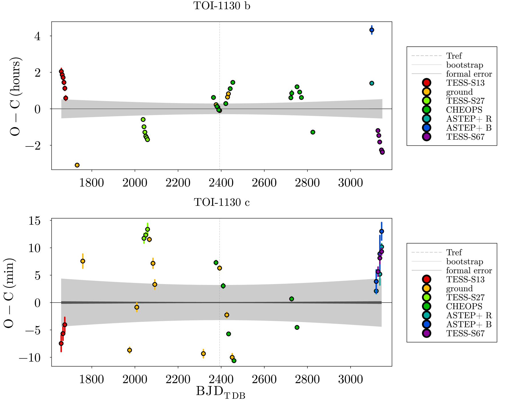
Figure 1: Observed minus Calculated (O-C) diagram of TOI-1130 b (top) and TOI-1130 c (bottom). The Calculated $T_{0}$s were determined from the linear ephemeris: $T_{\mathrm{lin,b,N}}=2392.81470\pm 0.00021\,(0.01260)+N\times 4.078668\pm 0.000002\,(0.000097)\,\mathrm{BTJD_{TDB}}$, and $T_{\mathrm{lin,c,N}}=2392.66995\pm 0.00007\,(0.00218)+N\times 8.349560\pm 0.000002\,(0.000023)\,\mathrm{BTJD_{TDB}}$, with formal (thin-black area) and bootstrap (between round brackets, gray area) uncertainty. Ground-based $T_{0}$s presented in Sec. 2.1.3 and analysed in Sec. 4.1 are reported as ground. $T_{\mathrm{ref}}$ is the reference time of the linear ephemeris plotted as dashed-gray vertical line. All the times are in BTJD, that is $\mathrm{BJD_{TDB}}-2\,457\,000$.

Then, we run a dynamical analysis with TRADES (Borsato et al. 2014, 2019, 2021) using as observable the $T_{0}$s and the boundaries for some parameters from the PyORBIT analysis. We let run TRADES with PyDE with a population of 96 parameter set for 90 000 generations. Differently from previous analysis, we let vary also the eccentricities, $e$ (and associated argument of pericenter, $\omega$), and held fix the radii and the inclination of the planets. Fitting parameters (e.g. $\sqrt{e}\cos\omega$ and $\sqrt{e}\sin\omega$), boundaries, and priors were defined as in Nascimbeni et al. (2023). At the end of the analysis we extracted the best-fit solution and computed the masses and physical parameters, that we used, jointly with PyORBIT results, as initial parameters for the successive photo-dynamical approach.

4.3 Photo-dynamical modelling

The photo-dynamical approach allows us to simultaneously fit the transit photometry (with detrending), transit times, and radial velocities, during the dynamical integration of the full system. An upgraded version of TRADES (photoTRADES) models transits with the PyTransit package (Parviainen 2015). The code integrates the orbits of the planets and computes all the possible transit times with associated Keplerian elements. Then, it automatically (and blindly) select the transit times and orbital elements of all the planets for each photometric portions, allowing us to model more planets for the same light curve portions, and pass them to PyTransit. It does not take into account for planet-planet (mutual) occultation. However, to reduce the computational time and the number of parameters, we decided to use the photometry (with detrending when needed) as in the PyORBIT analysis (see Sec. 4.2), and only the $T_{0}$s for the transit from ground-based facilities analysed in Sec. 4.1. For each radial velocity data-set we included an offset ($\gamma$) and jitter term (in $\log_{2}$), and a common linear trend in time (as in Korth et al. 2023) to take into account the possible influence of an additional planet on far outer orbit. See all 116 fitted parameters with boundaries and priors in Table LABEL:tab:phototrades.

We run photoTRADES with emcee with 232 walkers for $2\ 000\ 000$ steps with a thinning factor of 100. We discard the first $696\ 000$ steps as burn-in after checking the convergence of the chains through visual inspection and with Gelman-Rubin ($\hat{R}$), Geweke (Geweke 1991), and ACF statistics. As representative of the best-fit solution we took the maximum a posteriori (MAP), the parameter set that maximise the log-probability . Due to the high complexity of the problem, some MAP parameters (fitted or physical) are outside of the $1\sigma$ uncertainty defined as the high density interval (HDI) at the 68.27%. In this case, we computed and reported the HDI at the 95.44% as $2\sigma$ equivalent. See the full report of the fitted and physical parameters in Table LABEL:tab:phototrades. See $O-C$ diagram of the ground-based $T_{0}$s in Fig. 2, RV plot in Fig. 3, and photometry in Fig. 4 (with photometric residuals in Fig. 5).

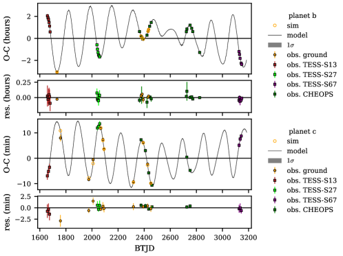
Figure 2: Observed minus Calculated ($O-C$) diagram of TOI-1130 b (top) and TOI-1130 c (bottom) from the photo-dynamical fit with TRADES of the ground-based $T_{0}$s (orange-black circles, simulated ones as open-orange circles) of photometry described in Sec. 4.1. The $O-C$ has been computed with the linear ephemeris in Table 3 and 4. Observed transit times of TESS and CHEOPS, not used in the fit, have been over-plotted (as colour-coded squares) on the $O-C$ and residual panels,

full MAP model as black line with $1\sigma$ gray-shaded area, that is almost invisible because the model is very well constrained. Times in $\mathrm{BTJD}=\mathrm{BJD_{TDB}}-2\,457\,000$.

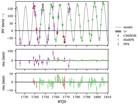
Figure 3: Radial velocity (subtracted RV offset, $\gamma$) plot in top panel with different marker and colour for each data-set. Observations as filled-markers and corresponding simulations as open-markers; full MAP model as black line with $1\sigma$ gray-shaded area. Residuals in mid-panel with all data-sets. Residuals without the CHIRON dataset in bottom-panel. Times in $\mathrm{BTJD}=\mathrm{BJD_{TDB}}-2\,457\,000$.

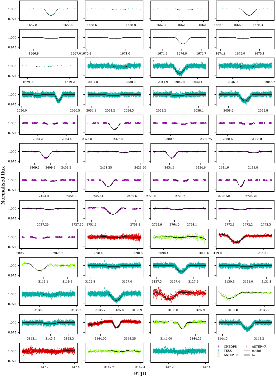
Figure 4: Photometry of each light curve used in the photo-dynamical analysis. Each panel has the data (filled markers, different marker and colour based on the facilities, see legend) with error-bars, and the over-plotted (over-sampled) full model (black line, transit and detrending) computed with the MAP parameter set from TRADES. Model uncertainties plotted as gray-shaded area at $1\sigma$, but barely visible. Times in $\mathrm{BTJD}=\mathrm{BJD_{TDB}}-2\,457\,000$.

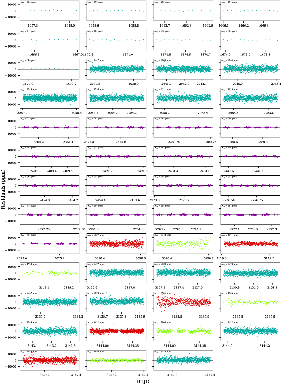
Figure 5: As in Fig. 4, but for the residuals (in ppm) between the observed photometry and the MAP full model. Each panel shows in the upper-left corner the standard deviation of the residuals in ppm.

We searched for additional signals in the Doppler data computing the generalised Lomb-Scargle periodogram (GLS, Zechmeister & Kürster 2009) of the HARPS and PFS RV residuals. We found no significant signals in the power spectrum, with the highest peak in the GLS periodogram having a relatively high false alarm probability (FAP) of $\sim$10%, as derived using a bootstrap randomisation approach with 10 000 repetitions (Hatzes 2019).

5 Discussions

5.1 Mean-Motion Resonance analysis

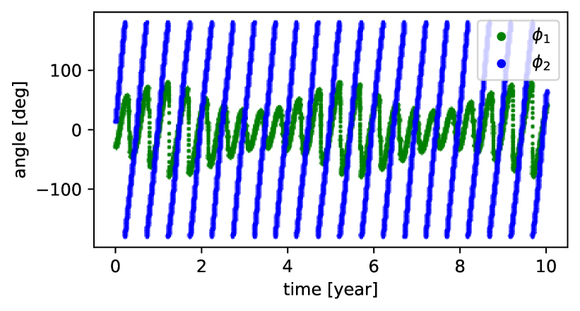
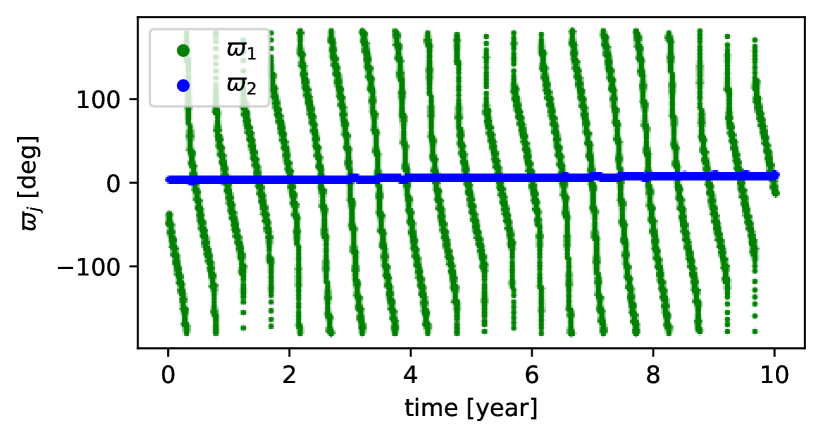
Figure 6: Example of evolution of the angles for a sample of the posterior. The top panel shows the resonant angles $\phi_{1}=\lambda_{1}-2\lambda_{2}+\varpi_{1}$ and $\phi_{2}=\lambda_{1}-2\lambda_{2}+\varpi_{2}$, where 1 refers to planet b and 2 to planet c, $\lambda$ is the mean longitude and $\varpi$ the longitude of periastron of the planets. The bottom panel shows the evolution of the longitude of periastron.

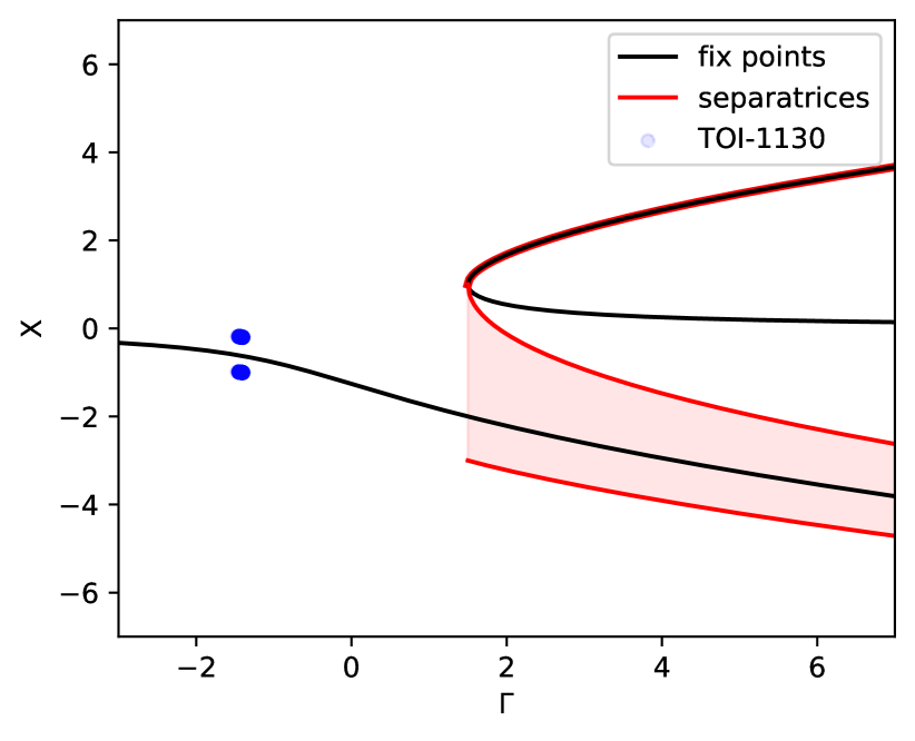
Figure 7: 1-degree of freedom model of the 2:1 MMR (Henrard & Lemaitre 1983; Deck et al. 2013). $X$ and $\Gamma$ are function of the orbital elements and masses of the system. $\Gamma$ represent how deep the system is in the resonance, while $X$ parameterise the position of the fix points and separatrices. The blue dots represent the intersection of 300 randomly-selected samples of the posterior with the $X$-$\Gamma$ plane.

For a pair of planets close enough to a first order mean-motion resonance (MMR), the expected TTVs is made of two terms: the evolution of the resonant angle ($\phi$), whose period is roughly proportional to $(m/m_{\star})^{-2/3}P_{\mathrm{orb}}$, where $m$ is comparable to the mass of the planets, and a slower term linked to the evolution of the eccentricities and longitude of periastron (Nesvorný & Vokrouhlický 2016). The relation between these two periods depend on the position of the system with respect to the exact resonance. Often, and in particular for smaller planets, an observation baseline of a few years only allow to observe the effect of the resonant angle, resulting in a mostly sinusoidal TTV signal. However, in the case of TOI-1130, the period of the two terms appear to be very close, with the period of precession of the inner orbit only slightly slower than the evolution of the resonant angle $\phi_{1}$, see Fig. 6. Adding up these two terms with similar period results in a TTV signal that appears to be modulated in amplitude, see Fig. 10.

The good constraints that we get for the resonant term of the TTVs allows us to constrain the resonant part of the architecture, as can be seen in Fig. 7. In that figure, we can see that the system lies outside the formal resonant domain (red area in the figure), unlike, for example, TOI-216 (Nesvorný et al. 2022). Observing the resonant term on its own does not allow to constrain the non-resonant part of the eccentricities, often resulting in a highly degenerated posterior for the eccentricities and longitudes of periastron (Leleu et al. 2021b, 2022, 2023). However, for TOI-1130, we can see the effect of the evolution of the periastron and the eccentricities on the TTVs, resulting in good constraints on these parameters.

Assuming that the pair was initially captured into the 2:1 due to a convergent migration in the proto-planetary disc (e.g. Weidenschilling & Davis 1985; Terquem & Papaloizou 2007), the observed architecture of the system enables in-depth study of its long term tidal evolution. Indeed, for planets whose orbital period is typically below 10 days, tides are expected to be an efficient mechanism to damp the eccentricity of the planet, effectively pushing the planets outside of the exact resonance (e.g. Novak et al. 2003; Lee et al. 2013; Delisle & Laskar 2014).

5.2 Internal Structure Modelling

We modelled the interior structure of TOI-1130 b using a Bayesian inference scheme, following the method introduced in Leleu et al. (2021a), which is based on Dorn et al. (2017). The forward model used is an early version of Haldemann et al. (2024) and uses equations of state from Hakim et al. (2018), Sotin et al. (2007) and Haldemann et al. (2020) to model each planet as a spherically symmetric structure made up of an inner iron core with up to 19% of sulphur, a silicate mantle made up of oxidised Si, Mg and Fe and a condensed water layer. On top of each such structure, a H/He envelope is modelled separately following Lopez & Fortney (2014). The elemental Si/Mg/Fe ratios are assumed to be stellar, following Thiabaud et al. (2015). While other studies find that at least for rocky planets this correlation might not be 1:1 (Adibekyan et al. 2021), the low density of TOI-1130 b, which means that it likely hosts a thick atmosphere, renders this assumption more reliable.

For the Bayesian inference, we use a uniform prior for the mass fractions of the inner core, mantle and water layer (on the simplex on which they add up to 1), with an upper limit of 0.5 for the water mass fraction (Thiabaud et al. 2014; Marboeuf et al. 2014). The mass of the H/He layer is sampled from a log-uniform prior. As the problem of modelling the internal structure of a planet is highly degenerate, the results of our analysis do depend to a certain extent on the chosen priors.

The resulting constraints on the internal structure of TOI-1130 b are summarised in Figure 8. According to our model, the planet hosts a H/He envelope with a mass of $M_{\mathrm{gas}}=0.62^{+0.43}_{-0.31}$ $M_{\oplus}$ and a thickness of $R_{\mathrm{gas}}=1.26_{-0.25}^{+0.27}\,R_{\oplus}$, where the values and errors correspond to the median and 5th and 95th percentiles of the posterior distributions. The presence and mass of a potential water layer remains fully unconstrained. However, these results are affected by our model only considering water in condensed form and modelling the H/He envelope independently from the rest of the planet, thereby neglecting any pressure and temperature effects it has on the rest of the planet.

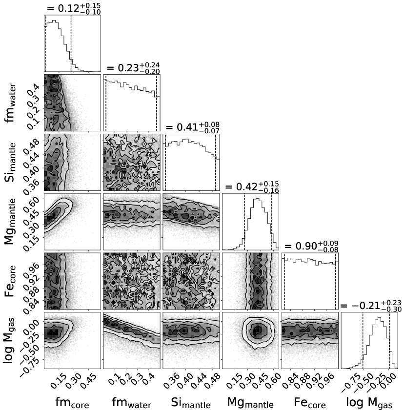
Figure 8: Inferred interior structure parameters of TOI-1130 b, with the values and errors above each histogram corresponding to the median and 5th and 95th percentile of each posterior distribution. The shown parameters are the mass fractions of the inner core and water layer (with respect to the solid part of the planet, they add up to 1 together with the mantle mass fraction), the elemental molar fractions of Si and Mg in the mantle and Fe in the inner core and the logarithm of the total H/He mass in Earth masses.

6 Conclusions

In this work we improved our knowledge on the multi-planet system TOI-1130 by re-analysing the whole transits and radial velocities presented in Korth et al. (2023) and with an additional TESS sector, six ground-based ASTEP+ transits, and 17 new high-precision photometric data observed with the CHEOPS satellite.

From the full photo-dynamical model with TRADES we obtained stellar parameters, $R_{\star}$, $\rho_{\star}$, and $M_{\star}$, within $1\sigma$ of our priors, but only $R_{\star}$ is consistent with the value derived by Korth et al. (2023). This could be due to (1) different priors used (parameters determined with different methods and codes), (2) different parameterisation (we fitted $R_{\star}$ and $\rho_{\star}$ instead of $R_{\star}$ and $M_{\star}$), (3) and longer baseline ($\sim 2$ yr) of additional photometric data with very-high precision CHEOPS light curves.

We found that $M_{\mathrm{b}}=19.8_{-0.3}^{+0.2}\,M_{\oplus}$, both radii ($R_{\mathrm{b}}=3.66_{-0.04}^{+0.03}\,R_{\oplus}$, $R_{\mathrm{c}}=13.0_{-0.4}^{+0.4}\,R_{\oplus}$) and densities ($\rho_{\mathrm{b}}=0.41_{-0.01}^{+0.01}\,\rho_{\oplus}$, $\rho_{\mathrm{c}}=0.15_{-0.02}^{+0.01}\,\rho_{\oplus}$) agree with Korth et al. (2023) within $1\sigma$, while $M_{\mathrm{c}}=336_{-5}^{+2}\,M_{\oplus}$ is consistent only at $2\sigma$. Thanks to CHEOPS light curves with very high photometric precision, and with additional ASTEP+ data, the determined precision of each parameter is higher than Korth et al. (2023), in particular $\sigma_{M_{\mathrm{b}}}\lesssim 1.5\%$, $\sigma_{R_{\mathrm{b}}}\lesssim 1.1\%$, $\sigma_{M_{\mathrm{c}}}\lesssim 1.5\%$, $\sigma_{R_{\mathrm{c}}}\lesssim 3\%$. Those values imply a precision of $\sim 3\%$ and $\sim 11\%$ on the densities of planet b and c, respectively. A comparison with Korth et al. (2023) values and other similar systems can be seen in the mass-radius relation in Fig. 9. We fitted eccentricities with flat-uniform priors in $(\sqrt{e}\cos\omega$, $\sqrt{e}\sin\omega)$ form and we also found that both planets have slightly eccentric orbits as suggested by Korth et al. (2023), but $e_{\mathrm{b}}$ is consistent within $2\sigma$, while we found a lower $e_{\mathrm{c}}$ consistent with their value only at $4\sigma$.

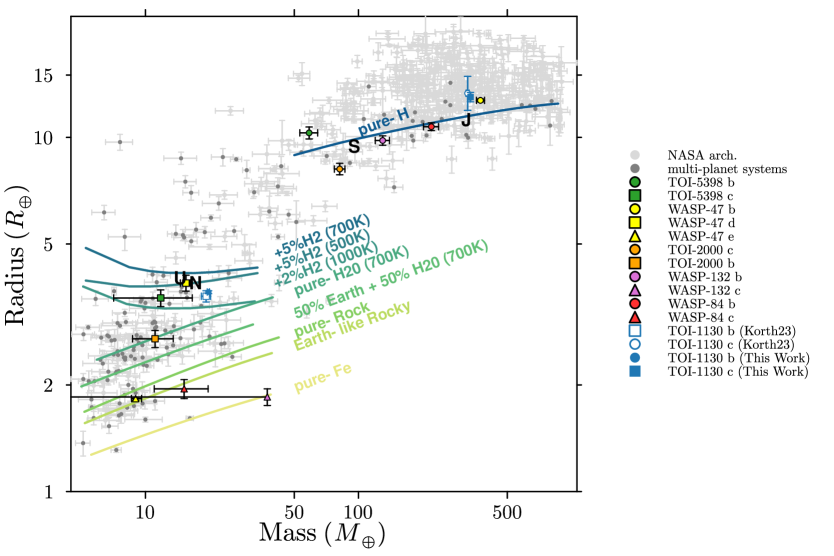
Figure 9: Mass-Radius relation plot with data from NASA Exoplanet archive for exoplanets with mass and radius precision lower than $20\%$. Models (plotted as color-coded lines) from Zeng et al. (2019) and https://lweb.cfa.harvard.edu/~lzeng/planetmodels.html#mrrelation. We plotted TOI-1130 b as square, white-fill blue-stroke from Korth et al. (2023) and full-blue from this work; TOI-1130 c as circle, same colour-code of TOI-1130 b. Over-plotted as darkgray circles the multi-planet systems and a sample of TOI-1130-like systems with different colours (based on host-name and with black outer stroke) and markers (based on planet type, circle for giants, triangle for $R_{\mathrm{p}}\leq 2\,R_{\oplus}$, and square in between): TOI-5398 (Mantovan et al. 2023), WASP-47 (Nascimbeni et al. 2023), TOI-2000 (Sha et al. 2023), WASP-132 (Hellier et al. 2017; Hord et al. 2022), and WASP-84 (Maciejewski et al. 2023). Over-plotted, also, Neptune (N), Uranus (U), Saturn (S), and Jupiter (J).

Although we were unable to fit for an additional outer planet due to the current data, we were able to tentatively estimate the minimum mass ($M_{\mathrm{d}}\sin i$) and semi-major axis ($a_{\mathrm{d}}$) of candidate planet d from the linear trend in the radial velocities. The period $P_{\mathrm{d}}$ was assumed to be 161.762 days, which is twice the total time spanned by the RV observations. Asymmetric Gaussian was generated for the stellar mass ($M_{\star}$) and RV linear trend from the photo-dynamical posterior. The expected linear RVs were computed for each generated RV linear trend, and the semi-amplitude $K_{\mathrm{RV}}$ was estimated as the difference between the maximum and minimum values. Inverting the equation $K_{\mathrm{RV}}\approx(M_{\mathrm{d}}\sin i)\ n\ a/M_{\star}$, with the mean motion $n=2\pi/P_{\mathrm{d}}$, and $a^{3}=GM_{\star}/n^{2}$, we found $a_{\mathrm{d}}=0.527\pm 0.002$ au and $M_{\mathrm{d}}\sin i=0.866_{-0.032}^{+0.025}\,M_{\mathrm{Jup}}$. However, these values strongly depend on the assumption that the period of this candidate is approximately twice the time elapsed during RV observations. Observing only a linear trend in the RV, it is possible that the period is longer, resulting in a higher mass. The GLS analysis of RV residuals of PFS and HARPS does not exhibit a significant signal (FAP$\sim 10\%$). Further radial velocity measurements would increase the temporal baseline needed to detect the correct period of the outer candidate.

The lower relative errors we obtained in the orbital parameters allows us to predict the future transit times (see the O-C diagram in Fig. 10), until 2028, with a very high precision ($\sigma_{T_{0},\mathrm{max}}=2.6$ min and $20$ s for planet b and c, respectively). This is very important because the precise knowledge of when both planets transit is of fundamental importance for the upcoming transmission spectroscopy observations with JWST (Gardner et al. 2023) and Ariel (Tinetti et al. 2018). In fact, TOI-1130 c is one of the planets with the highest Transmission Spectroscopic Metric (TSM, Kempton et al. 2018), and both planets are part of a JWST proposal. JWST and Ariel observations will allow us to characterise atmospheric abundances which are, as suggested by Korth et al. (2023), crucial to understand the formation process that the system underwent.

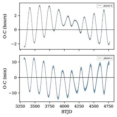
Figure 10: O-C diagram of the synthetic $T_{0}$s predicted with the MAP orbital solution (black dots connected by black line) from photo-TRADES analysis. Uncertainty plotted as $3\sigma$ in dark-blue, $2\sigma$ in light-blue, and $1\sigma$ whitish-blue. The $x$-axis in $\mathrm{BTJD}=\mathrm{BJD_{TDB}}-2\,457\,000$ ranges from 2024 until 2028.

Data Availability

Data will be available at CDS. Data type: Observed-Fitted transit times in ascii file. ASTEP+ and CHEOPS-PIPE data and best-fit model in ascii file. Predicted transit times from 2024 to 2028 in ascii file.

References

- Adibekyan et al. (2021) Adibekyan, V., Dorn, C., Sousa, S. G., et al. 2021, Science, 374, 330
- Agol et al. (2020) Agol, E., Luger, R., & Foreman-Mackey, D. 2020, AJ, 159, 123
- Agol et al. (2005) Agol, E., Steffen, J., Sari, R., & Clarkson, W. 2005, MNRAS, 359, 567
- Barnes (2010) Barnes, S. A. 2010, ApJ, 722, 222
- Baruteau et al. (2016) Baruteau, C., Bai, X., Mordasini, C., & Mollière, P. 2016, Space Sci. Rev., 205, 77
- Becker et al. (2015) Becker, J. C., Vanderburg, A., Adams, F. C., Rappaport, S. A., & Schwengeler, H. M. 2015, ApJ, 812, L18
- Benz et al. (2021) Benz, W., Broeg, C., Fortier, A., et al. 2021, Experimental Astronomy, 51, 109
- Bezanson et al. (2017) Bezanson, J., Edelman, A., Karpinski, S., & Shah, V. B. 2017, SIAM review, 59, 65
- Blackwell & Shallis (1977) Blackwell, D. E. & Shallis, M. J. 1977, MNRAS, 180, 177
- Bonfanti et al. (2021) Bonfanti, A., Delrez, L., Hooton, M. J., et al. 2021, arXiv e-prints, arXiv:2101.00663
- Bonfanti et al. (2016) Bonfanti, A., Ortolani, S., & Nascimbeni, V. 2016, A&A, 585, A5
- Bonfanti et al. (2015) Bonfanti, A., Ortolani, S., Piotto, G., & Nascimbeni, V. 2015, A&A, 575, A18
- Borsato et al. (2019) Borsato, L., Malavolta, L., Piotto, G., et al. 2019, MNRAS, 484, 3233
- Borsato et al. (2014) Borsato, L., Marzari, F., Nascimbeni, V., et al. 2014, A&A, 571, A38
- Borsato et al. (2021) Borsato, L., Piotto, G., Gandolfi, D., et al. 2021, MNRAS, 506, 3810
- Brandeker et al. (2022) Brandeker, A., Heng, K., Lendl, M., et al. 2022, A&A, 659, L4
- Bryant & Bayliss (2022) Bryant, E. M. & Bayliss, D. 2022, AJ, 163, 197
- Cañas et al. (2019) Cañas, C. I., Wang, S., Mahadevan, S., et al. 2019, ApJ, 870, L17
- Castelli & Kurucz (2003) Castelli, F. & Kurucz, R. L. 2003, in IAU Symposium, Vol. 210, Modelling of Stellar Atmospheres, ed. N. Piskunov, W. W. Weiss, & D. F. Gray, A20
- Chatterjee et al. (2008) Chatterjee, S., Ford, E. B., Matsumura, S., & Rasio, F. A. 2008, ApJ, 686, 580
- Claret (2017) Claret, A. 2017, Astronomy & Astrophysics, 600, A30
- Collaboration et al. (2018) Collaboration, A., Price-Whelan, A. M., Sipőcz, B. M., et al. 2018, AJ, 156, 123
- Collaboration et al. (2013) Collaboration, A., Robitaille, T. P., Tollerud, E. J., et al. 2013, A&A, 558, A33
- Crane et al. (2006) Crane, J. D., Shectman, S. A., & Butler, R. P. 2006, in Society of Photo-Optical Instrumentation Engineers (SPIE) Conference Series, Vol. 6269, Society of Photo-Optical Instrumentation Engineers (SPIE) Conference Series, ed. I. S. McLean & M. Iye, 626931
- Crane et al. (2010) Crane, J. D., Shectman, S. A., Butler, R. P., et al. 2010, in Society of Photo-Optical Instrumentation Engineers (SPIE) Conference Series, Vol. 7735, Ground-based and Airborne Instrumentation for Astronomy III, ed. I. S. McLean, S. K. Ramsay, & H. Takami, 773553
- Crane et al. (2008) Crane, J. D., Shectman, S. A., Butler, R. P., Thompson, I. B., & Burley, G. S. 2008, in Society of Photo-Optical Instrumentation Engineers (SPIE) Conference Series, Vol. 7014, Ground-based and Airborne Instrumentation for Astronomy II, ed. I. S. McLean & M. M. Casali, 701479
- Deck et al. (2013) Deck, K. M., Payne, M., & Holman, M. J. 2013, ApJ, 774, 129
- Degen (2022) Degen, D. 2022, Master’s thesis, Eidgenössische Technische Hochschule Zürich (ETHZ)
- Delisle & Laskar (2014) Delisle, J. B. & Laskar, J. 2014, A&A, 570, L7
- Dorn et al. (2017) Dorn, C., Venturini, J., Khan, A., et al. 2017, A&A, 597, A37
- Foreman-Mackey et al. (2019) Foreman-Mackey, D., Farr, W., Sinha, M., et al. 2019, The Journal of Open Source Software, 4, 1864
- Foreman-Mackey et al. (2013) Foreman-Mackey, D., Hogg, D. W., Lang, D., & Goodman, J. 2013, PASP, 125, 306
- Foreman-Mackey et al. (2021a) Foreman-Mackey, D., Luger, R., Agol, E., et al. 2021a, The Journal of Open Source Software, 6, 3285
- Foreman-Mackey et al. (2021b) Foreman-Mackey, D., Savel, A., Luger, R., et al. 2021b, exoplanet-dev/exoplanet v0.5.1
- Gaia Collaboration et al. (2022) Gaia Collaboration, Vallenari, A., Brown, A. G. A., et al. 2022, arXiv e-prints, arXiv:2208.00211
- Gardner et al. (2023) Gardner, J. P., Mather, J. C., Abbott, R., et al. 2023, PASP, 135, 068001
- Gelman & Rubin (1992) Gelman, A. & Rubin, D. B. 1992, Statistical Science, 7, 457
- Geweke (1991) Geweke, J. F. 1991, Evaluating the accuracy of sampling-based approaches to the calculation of posterior moments, Staff Report 148, Federal Reserve Bank of Minneapolis
- Gray (2008) Gray, D. F. 2008, The Observation and Analysis of Stellar Photospheres (Cambridge University Press)
- Guillot et al. (2015) Guillot, T., Abe, L., Agabi, A., et al. 2015, Astronomische Nachrichten, 336, 638
- Gustafsson et al. (2008) Gustafsson, B., Edvardsson, B., Eriksson, K., et al. 2008, A&A, 486, 951
- Hakim et al. (2018) Hakim, K., Rivoldini, A., Van Hoolst, T., et al. 2018, Icarus, 313, 61
- Haldemann et al. (2020) Haldemann, J., Alibert, Y., Mordasini, C., & Benz, W. 2020, A&A, 643, A105
- Haldemann et al. (2024) Haldemann, J., Dorn, C., Venturini, J., Alibert, Y., & Benz, W. 2024, A&A, 681, A96
- Harris et al. (2020) Harris, C. R., Millman, K. J., van der Walt, S. J., et al. 2020, Nature, 585, 357–362
- Hatzes (2019) Hatzes, A. P. 2019, The Doppler Method for the Detection of Exoplanets, 2514-3433 (IOP Publishing)
- Hellier et al. (2017) Hellier, C., Anderson, D. R., Collier Cameron, A., et al. 2017, MNRAS, 465, 3693
- Hellier et al. (2012) Hellier, C., Anderson, D. R., Collier Cameron, A., et al. 2012, MNRAS, 426, 739
- Henrard & Lemaitre (1983) Henrard, J. & Lemaitre, A. 1983, Celestial Mechanics, 30, 197
- Holman & Murray (2005) Holman, M. J. & Murray, N. W. 2005, Science, 307, 1288
- Hord et al. (2022) Hord, B. J., Colón, K. D., Berger, T. A., et al. 2022, AJ, 164, 13
- Hoyer et al. (2020) Hoyer, S., Guterman, P., Demangeon, O., et al. 2020, A&A, 635, A24
- Huang et al. (2023) Huang, C., Vanderburg, A., Korth, J., et al. 2023, The first comparative atmospheric study of a Jovian planet and a sub-Neptune in the TOI-1130 system, JWST Proposal. Cycle 2, ID. #3385
- Huang et al. (2016) Huang, C., Wu, Y., & Triaud, A. H. M. J. 2016, ApJ, 825, 98
- Huang et al. (2020a) Huang, C. X., Quinn, S. N., Vanderburg, A., et al. 2020a, ApJ, 892, L7
- Huang et al. (2020b) Huang, C. X., Vanderburg, A., Pál, A., et al. 2020b, Research Notes of the American Astronomical Society, 4, 204
- Hunter (2007) Hunter, J. D. 2007, Computing in science & engineering, 9, 90
- Husser et al. (2013) Husser, T.-O., Wende-von Berg, S., Dreizler, S., et al. 2013, A&A, 553, A6
- Jackson et al. (2023) Jackson, J. M., Dawson, R. I., Quarles, B., & Dong, J. 2023, AJ, 165, 82
- Jenkins et al. (2016) Jenkins, J. M., Twicken, J. D., McCauliff, S., et al. 2016, in Society of Photo-Optical Instrumentation Engineers (SPIE) Conference Series, Vol. 9913, Software and Cyberinfrastructure for Astronomy IV, 99133E
- Kempton et al. (2018) Kempton, E. M. R., Bean, J. L., Louie, D. R., et al. 2018, PASP, 130, 114401
- Kipping (2013) Kipping, D. M. 2013, MNRAS, 435, 2152
- Kley (2019) Kley, W. 2019, Planet Formation and Disk-Planet Interactions, ed. M. Audard, M. R. Meyer, & Y. Alibert (Berlin, Heidelberg: Springer Berlin Heidelberg), 151–260
- Korth et al. (2023) Korth, J., Gandolfi, D., Šubjak, J., et al. 2023, A&A, 675, A115
- Kreidberg (2015) Kreidberg, L. 2015, PASP, 127, 1161
- Kumar et al. (2019) Kumar, R., Carroll, C., Hartikainen, A., & Martin, O. 2019, The Journal of Open Source Software, 4, 1143
- Kurucz (2013) Kurucz, R. L. 2013, ATLAS12: Opacity sampling model atmosphere program, Astrophysics Source Code Library
- Latham et al. (2011) Latham, D. W., Rowe, J. F., Quinn, S. N., et al. 2011, ApJ, 732, L24
- Lee et al. (2013) Lee, M. H., Fabrycky, D., & Lin, D. N. C. 2013, ApJ, 774, 52
- Leleu et al. (2021a) Leleu, A., Alibert, Y., Hara, N. C., et al. 2021a, A&A, 649, A26
- Leleu et al. (2021b) Leleu, A., Chatel, G., Udry, S., et al. 2021b, A&A, 655, A66
- Leleu et al. (2022) Leleu, A., Delisle, J. B., Mardling, R., et al. 2022, A&A, 661, A141
- Leleu et al. (2023) Leleu, A., Delisle, J. B., Udry, S., et al. 2023, A&A, 669, A117
- Lin et al. (1996) Lin, D. N. C., Bodenheimer, P., & Richardson, D. C. 1996, Nature, 380, 606
- Lindegren et al. (2021) Lindegren, L., Bastian, U., Biermann, M., et al. 2021, A&A, 649, A4
- Lopez & Fortney (2014) Lopez, E. D. & Fortney, J. J. 2014, ApJ, 792, 1
- Luger et al. (2019) Luger, R., Agol, E., Foreman-Mackey, D., et al. 2019, AJ, 157, 64
- Maciejewski et al. (2023) Maciejewski, G., Golonka, J., Łoboda, W., et al. 2023, MNRAS, 525, L43
- Malavolta et al. (2018) Malavolta, L., Mayo, A. W., Louden, T., et al. 2018, AJ, 155, 107
- Malavolta et al. (2016) Malavolta, L., Nascimbeni, V., Piotto, G., et al. 2016, A&A, 588, A118
- Mantovan et al. (2023) Mantovan, G., Malavolta, L., Desidera, S., et al. 2023, arXiv e-prints, arXiv:2310.16888
- Mantovan et al. (2022) Mantovan, G., Montalto, M., Piotto, G., et al. 2022, MNRAS, 516, 4432
- Marboeuf et al. (2014) Marboeuf, U., Thiabaud, A., Alibert, Y., Cabral, N., & Benz, W. 2014, A&A, 570, A36
- Marigo et al. (2017) Marigo, P., Girardi, L., Bressan, A., et al. 2017, ApJ, 835, 77
- Maxted et al. (2022) Maxted, P. F. L., Ehrenreich, D., Wilson, T. G., et al. 2022, MNRAS, 514, 77
- Mayor et al. (2003) Mayor, M., Pepe, F., Queloz, D., et al. 2003, The Messenger, 114, 20
- Mékarnia et al. (2016) Mékarnia, D., Guillot, T., Rivet, J. P., et al. 2016, MNRAS, 463, 45
- Moré et al. (1980) Moré, J. J., Garbow, B. S., & Hillstrom, K. E. 1980, User guide for MINPACK-1, Tech. Rep. ANL-80-74, Argonne Nat. Lab., Argonne, IL
- Morris et al. (2021) Morris, B. M., Delrez, L., Brandeker, A., et al. 2021, A&A, 653, A173
- Nagasawa et al. (2008) Nagasawa, M., Ida, S., & Bessho, T. 2008, ApJ, 678, 498
- Nascimbeni et al. (2023) Nascimbeni, V., Borsato, L., Zingales, T., et al. 2023, A&A, 673, A42
- Nesvorný et al. (2022) Nesvorný, D., Chrenko, O., & Flock, M. 2022, ApJ, 925, 38
- Nesvorný & Vokrouhlický (2016) Nesvorný, D. & Vokrouhlický, D. 2016, ApJ, 823, 72
- Novak et al. (2003) Novak, G. S., Lai, D., & Lin, D. N. C. 2003, in Astronomical Society of the Pacific Conference Series, Vol. 294, Scientific Frontiers in Research on Extrasolar Planets, ed. D. Deming & S. Seager, 177–180
- Parviainen (2015) Parviainen, H. 2015, MNRAS, 450, 3233
- Parviainen & Aigrain (2015) Parviainen, H. & Aigrain, S. 2015, MNRAS, 453, 3821
- Parviainen et al. (2016) Parviainen, H., Pallé, E., Nortmann, L., et al. 2016, A&A, 585, A114
- Persson et al. (2018) Persson, C. M., Fridlund, M., Barragán, O., et al. 2018, A&A, 618, A33
- Piskunov & Valenti (2017) Piskunov, N. & Valenti, J. A. 2017, A&A, 597, A16
- Rasio & Ford (1996) Rasio, F. A. & Ford, E. B. 1996, Science, 274, 954
- Ricker et al. (2015) Ricker, G. R., Winn, J. N., Vanderspek, R., et al. 2015, Journal of Astronomical Telescopes, Instruments, and Systems, 1, 014003
- Ryabchikova et al. (2015) Ryabchikova, T., Piskunov, N., Kurucz, R. L., et al. 2015, Phys. Scr, 90, 054005
- Salmon et al. (2021) Salmon, S. J. A. J., Van Grootel, V., Buldgen, G., Dupret, M. A., & Eggenberger, P. 2021, A&A, 646, A7
- Salvatier et al. (2015) Salvatier, J., Wiecki, T., & Fonnesbeck, C. 2015, arXiv e-prints, arXiv:1507.08050
- Schanche et al. (2020) Schanche, N., Hébrard, G., Collier Cameron, A., et al. 2020, MNRAS, 499, 428
- Schlaufman & Winn (2016) Schlaufman, K. C. & Winn, J. N. 2016, ApJ, 825, 62
- Schmider et al. (2022) Schmider, F.-X., Abe, L., Agabi, A., et al. 2022, in Society of Photo-Optical Instrumentation Engineers (SPIE) Conference Series, Vol. 12182, Ground-based and Airborne Telescopes IX, ed. H. K. Marshall, J. Spyromilio, & T. Usuda, 121822O
- Scuflaire et al. (2008) Scuflaire, R., Théado, S., Montalbán, J., et al. 2008, Ap&SS, 316, 83
- Sha et al. (2023) Sha, L., Vanderburg, A. M., Huang, C. X., et al. 2023, MNRAS, 524, 1113
- Skrutskie et al. (2006) Skrutskie, M. F., Cutri, R. M., Stiening, R., et al. 2006, AJ, 131, 1163
- Sotin et al. (2007) Sotin, C., Grasset, O., & Mocquet, A. 2007, Icarus, 191, 337
- Steffen et al. (2012) Steffen, J. H., Ragozzine, D., Fabrycky, D. C., et al. 2012, Proceedings of the National Academy of Science, 109, 7982
- Storn & Price (1997) Storn, R. & Price, K. V. 1997, J. Glob. Optim., 11, 341
- Team et al. (2016) Team, T. T. D., Al-Rfou, R., Alain, G., et al. 2016, arXiv e-prints, arXiv:1605.02688
- Terquem & Papaloizou (2007) Terquem, C. & Papaloizou, J. C. B. 2007, ApJ, 654, 1110
- Thiabaud et al. (2014) Thiabaud, A., Marboeuf, U., Alibert, Y., et al. 2014, A&A, 562, A27
- Thiabaud et al. (2015) Thiabaud, A., Marboeuf, U., Alibert, Y., Leya, I., & Mezger, K. 2015, A&A, 574, A138
- Tinetti et al. (2018) Tinetti, G., Drossart, P., Eccleston, P., et al. 2018, Experimental Astronomy, 46, 135
- Tokovinin et al. (2013) Tokovinin, A., Fischer, D. A., Bonati, M., et al. 2013, PASP, 125, 1336
- Tommasini & Olivieri (2021) Tommasini, D. & Olivieri, D. N. 2021, MNRAS, 506, 1889
- Valenti & Piskunov (1996) Valenti, J. A. & Piskunov, N. 1996, A&AS, 118, 595
- Vick et al. (2019) Vick, M., Lai, D., & Anderson, K. R. 2019, MNRAS, 484, 5645
- Vick et al. (2023) Vick, M., Su, Y., & Lai, D. 2023, ApJ, 943, L13
- Virtanen et al. (2020) Virtanen, P., Gommers, R., Oliphant, T. E., et al. 2020, Nature Methods, 17, 261
- Weidenschilling & Davis (1985) Weidenschilling, S. J. & Davis, D. R. 1985, Icarus, 62, 16
- Wright et al. (2010) Wright, E. L., Eisenhardt, P. R. M., Mainzer, A. K., et al. 2010, AJ, 140, 1868
- Wu et al. (2018) Wu, D.-H., Wang, S., Zhou, J.-L., Steffen, J. H., & Laughlin, G. 2018, AJ, 156, 96
- Yee et al. (2017) Yee, S. W., Petigura, E. A., & von Braun, K. 2017, ApJ, 836, 77
- Zechmeister & Kürster (2009) Zechmeister, M. & Kürster, M. 2009, A&A, 496, 577
- Zeng et al. (2019) Zeng, L., Jacobsen, S. B., Sasselov, D. D., et al. 2019, Proceedings of the National Academy of Science, 116, 9723
- Zhu et al. (2018) Zhu, W., Dai, F., & Masuda, K. 2018, Research Notes of the American Astronomical Society, 2, 160