Freezing and Shielding under Global Quenches for Long-Range Interacting Many-Body Systems

Abstract

We investigate the time evolution of a Fermi-Hubbard model with long range hopping following a sudden quench of the local interactions among different spin species. The quasi-particle spectrum consists of gapped low-energy levels while the high energy modes accumulate at a single point. When the low energy gaps are large enough, turning on the local interactions does not effectively mix high and low energy modes, leading to the freezing of the dynamical evolution. In general, the states within the excited subspace are shielded from the long-range signatures of the model, which are responsible for the low energy extended states, and the dynamics effectively look as if long-range hopping were absent. This cooperative shielding mechanism becomes evident in presence of disorder. It is shown that shielding and freezing are a universal feature of long-range interacting systems and conjecture that they are related to the existence of quasi-stationary states.

Introduction: Modern advances in the realization of experimental quantum platforms have unveiled thrilling avenues for exploring the non-equilibrium dynamics of complex systems, whose Hamiltonian can be effectively simulated on these platforms. Their high degree of flexibility enables rapid changes of the interaction parameters of the underlying effective model and permits the study the subsequent dynamics. Moreover, the near-perfect isolation of several quantum platforms from external influences allows the dynamics of the effective system to remain coherent for long periods [1]. This has prompted the study of how isolated many-body quantum systems thermalize, a question of great interest in theoretical physics, whose answer promises to boost important developments in quantum technology [2].

The flexibility of current experimental quantum platforms does not only allow to address the out-of-equilibrium dynamics, but often allows to also tailor the interaction shape. Out of this exciting possibility, a great interest has spurred in the physics of long-range interacting quantum systems [3]. Conventionally, the term long-range denotes couplings decaying as $1/r^{\alpha}$ (where $r$ is the distance between two components of the many-body system under study). Depending on the dimension of the system $d$, one defines three regimes: i) the local regime $\alpha>\alpha_{*}$, where $\alpha_{*}$ is a system and phenomenon dependent threshold beyond which nearest-neighbour or local physics is recovered; ii) the weak long-range regime ($d<\alpha<\alpha_{*}$) where long-range interactions are relevant, but thermodynamics functions remain extensive; iii) finally, for $0<\alpha<d$ the strong long-range regime appears where conventional thermodynamics becomes ill-defined [4]. Long-range quantum systems count several practical realisation including Rydberg atom arrays [5], dipolar systems [6, 7], trapped ion setups [8] and cold atoms in cavity experiments [9, 10, 11] and are key candidates for the realization of efficient quantum computing devices [12].

Strong long-range interactions enable a plethora of exciting out-of-equilibrium phenomena. One of their distinct feature in classical systems is the presence of pre-thermal phases denoted as quasi-stationary states (QSSs), whose lifetimes increase with the system size [13]. In the quantum realm, QSSs were first demonstrated in theory, showing diverging equilibration times for isolated long-range quantum systems [14] and long-lived prethermal states generated by cavity-mediated long-range interactions [15], where dissipation also plays a role [16]. Experimental evidences of the analogy between isolated long-range many-body systems and quantum gases in cavities were recently obtained by investigating the dynamical evolution of a degenerate Fermi gas in a cavity [11].

The peculiarity of long-range out-of-equilibrium dynamics is not confined to QSSs. In Ref. [17, 18] it was observed that, even in presence of strong long-range interactions, the dynamics is governed by an emergent short-range Hamiltonian, at least for initial states within specific subsets of the Hilbert space. In this case, the spreading of perturbation is confined to an effective light cone, as defined by the local Lieb-Robinson bound [19] and it deviates from the general expectations for long range interactions [20]. More recently, it was shown [21] that the long-range interacting Ising chain also supports quantum many-body scars, intended as isolated states in the many-body spectrum which are associated with lack of thermalization in the system. Interestingly, the theoretical arguments of the Refs. [17, 18, 21] are based on the exact solution of the flat interacting case at $\alpha=0$, which is then extended to finite $\alpha<d$ thanks to perturbative arguments.

In the present work, we intend to provide solid evidences for the universality of the shielding phenomenon as well as to give further indications for the lack of thermalization produced by long-range interactions. Our approach is complementary to previous studies concerning two main aspects:

1. the shielding phenomenon is shown to be universal as it occurs on equal footing for all values of $\alpha$ and it can be traced back to the overall properties of the weakly interacting quasi-particle spectrum.

2. the study is performed for global quenches of the interacting Hamiltonian rather than the local quenches [17, 18] enlarging the applicability of the concept of “shielding”.

3. the system under consideration are constituted by fermionic particles rather than spins, possibly allowing for a more direct connection to the ongoing experiments [11].

More in general, our study aims at creating a wider understanding of the peculiarities of long-range dynamics in terms of their unique spectral properties [22].

In order to provide solid arguments to the above statements we focus on a paradigmatic model of correlated electrons frequently studied in the literature, i.e. the repulsive Hubbard model in $d=1$ [23]. The core aspects which make this system the ideal playground for our study are (i) the existence of a wide range of established tools to approximately study it’s dynamics, in particular dynamical mean-field theory (DMFT) [24, 25, 26, 27, 28], and the existence of a well defined quasi-particle limit at weak interactions $U\approx 0$.

In our case, we analyse the dynamics of the Hubbard model, where the fermions display long-range hopping amplitudes, after the local interaction is suddenly ignited in the whole system. For purely long-range couplings the system’s observables remain mostly unchanged after the quench, a phenomenon often referred to as freezing. We analytically connect the existence of the freezing phenomenon with the survival of the low-energy single-particle spectral gaps and to the appearance of an high-energy accumulation point in the quasi-particle spectrum due to long-range hopping amplitudes.

Once Gaussian disorder is introduced in the couplings, the degeneracy of the accumulation point is lifted, generating the celebrated semi-circular density of states observed in Gaussian random matrices [29]. The appearance of the continuous spectrum unfreezes the dynamics, but the effect of long-range couplings remain confined to few low-energy discrete states, whose very limited impact on the global dynamics leads to the phenomenon of shielding. These dynamical effects can be demonstrated exactly only in the thermodynamic limit, highlighting the cooperative nature of the shielding and freezing mechanism. Finally, we discuss the differences between re-scaled and un-scaled long range interactions under Kac’s prescription and determine their effect in the dynamics of fermionic systems [30].

The model: the Fermi-Hubbard model describes Fermi particles hopping between the $L$ sites of a 1-dimensional lattice. We consider its generalization where the hopping amplitudes are long-range and periodic boundary conditions are taken

$$H_{0}=-\sum_{i=1}^{L}\sum_{r=1}^{L/2-1}t_{r}\left(\hat{c}^{\dagger}_{i\sigma}\hat{c}_{i+r\sigma}+\text{h.c.}\right)+\mu\sum_{i=1}^{L}\hat{c}^{\dagger}_{i}\hat{c}_{i},$$ (1a)

$$H_{\text{int}}=U\sum_{i=1}^{L}\hat{n}_{i\uparrow}\hat{n}_{i\downarrow},$$ (1b)

and the total Hamiltonian is $H=H_{0}+H_{\text{int}}$. In addition to the conventional long-range envelope, we allow the hopping amplitude $t_{r}$ to fluctuate around a mean-value that decays as a power-law of the distance. Apart from being an important tool to explore the theoretical physics of the model, the addition of disorder is useful to account for the inherent uncertainty of the hopping amplitudes between the local Wannier states in a tight binding model. The probability distribution of each $t_{r}$ is an independent Gaussian distribution with finite mean and variance,

$$\braket{t_{r}}=\frac{M_{\alpha}}{r^{\alpha}},\hskip 28.45274pt\braket{t_{r}t_{r^{\prime}}}=\sigma^{2}\delta_{rr^{\prime}}\equiv\frac{J^{2}}{L^{2}}\delta_{rr^{\prime}}$$ (2)

At this point we would like to nail down whether we require for a re-scaling of the amplitudes to ensure extensivity of the energy. Let us examine the simplest case where $\alpha=0$ and $\sigma\rightarrow 0$. In this case, there is no disorder and the kinetic energy is solely carried by the zero momentum mode $\epsilon_{k}=-LM_{\alpha}\hat{c}^{\dagger}_{k}\hat{c}_{k}\delta_{k0}$. For bosons, where condensation can occur, the divergence of the zero-mode energy introduces the necessity to re-scale the hopping to ensure that the kinetic energy remains extensive on the thermodynamic limit, a procedure refereed to as Kac re-scaling [3]. The fermionic case is different as only a single fermion can occupy the zero-momentum mode leading to sub-extensive kinetic energy in the presence of Kac scaling. However, in order to draw connections with most of the existing literature, we will consider both Kac-scaled and un-scaled strong long-range interactions.

Apart from the single zero momentum mode with super-extensive energy, the $\alpha=0$ quasi-particle spectrum features a $N-1$ degenerate state with energy $\varepsilon_{k>0}=\mu$, which we refer to as the high-energy accumulation point [31]. Again for flat couplings and vanishing interactions, $\alpha=U=0$, a finite disorder strength $\sigma>0$ lifts the high energy degeneracy leading to a continuous spectrum with semi-circular shape plus the isolated state low-energy $k=0$ mode, in analogy with the problem of a single impurity in a crystal [32]. Similarly, for $0\leq\alpha<1$, the presence of disorder mixes the high energy states and transforms the accumulation point into a continuum of energy-levels distributed according to Wigner’s semi-circle law. However, the discrete low-energy levels survives as long as their energies reside outside the semi-circle radius . Then, the density of states takes the generic form valid at any $\alpha$,

$$\rho(\lambda)=\frac{\sqrt{4J^{2}-\lambda^{2}}}{2\pi J^{2}}+\frac{1}{L}\sum_{n<n^{*}}\delta(\lambda-\lambda_{n})$$ (3)

where $\lambda_{n}=M_{\alpha}\epsilon_{n}+J^{2}/(M_{\alpha}\epsilon_{n})$ and $\epsilon_{n}$ corresponds to the eigen-energies of the free long-range hopping model ($\alpha<1$) in the absence of disorder. In this case $n\in\mathbb{Z}$ and $-L/2\leq n<L/2$,

$$\epsilon_{n}=-\sum_{r=1}^{L/2}\frac{\cos(2\pi nr/N)}{r^{\alpha}}=-c_{\alpha}\int_{0}^{1/2}ds\frac{\cos\left(2\pi ks\right)}{s^{\alpha}}.$$ (4a)

Here $c_{\alpha}$ may or not contain a Kac’s renormalization factor, depending on the case under study

$$c_{\alpha}=\begin{cases}(1-\alpha)2^{(1-\alpha)}N^{\alpha-1}&\qquad\mathrm{Kac\,\,on}\\ 1&\qquad\mathrm{Kac\,\,off}\end{cases}$$ (5)

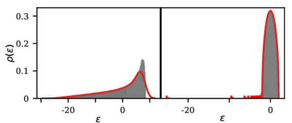
Figure 1: Density of states with Gaussian disorder Eq. (2) for $\alpha=1.5$ (left panel) and $\alpha=0.5$ (right one) for $M_{0}=-4\pi$ and $\sigma=1$. Shaded are corresponds to an histogram of the eigenvalues for $L=2^{13}$ while the continuous red line is the density of states in absence of disorder in the $\alpha=1.5$ panel and our analytical prediction in the $\alpha=0.5$ one. We observe the appearance of the semi-circular profile only for strong long-range interactions $\alpha<d$.

Eq. (16) summarizes the interplay of disorder and long-range couplings in the single particle spectrum. The spectral discreteness typical of long-range interactions persists under the presence of disorder, but coexists with a continuous portion of the spectrum which originates due to the splitting of the high-energy accumulation point. Indeed, in Fig. 1 we can see how the effect of disorder only changes the high energy tails of the density of states (DOS). For $\alpha<1$ the density of states is correctly described by Eq.(16) while for $\alpha>1$ there is no semi-circular profile and the DOS resembles the clean case up to really high energies.

Shielding and freezing: both these phenomena occur in the strong long-range regime, and so in the following, we focus on $\alpha<d$. Initially, the system is prepared in the non-interacting ground-state, i.e. the lowest energy state of the Hamiltonian $H_{0}$. This corresponds to a Fermi sea, where single particle states are occupied up to the $N_{\uparrow}=N_{\downarrow}=L/2$ level (half-filling), and $N_{\uparrow(\downarrow)}$ is the number of up(down) electrons. It is worth noting that the spin population is conserved during the dynamics. In order to fix the electron density at half-filling, the chemical potential of the clean long-range Fermi-Hubbard must lie at the high energy-accumulation point. As already mentioned, the inclusion of disorder spreads such accumulation point and generates the semicircular DOS depicted in Fig. 1; accordingly, the chemical potential has to be modified in order to maintain the electron density at half-filling in the thermodynamic limit.

At $t=0$ the onsite interaction is suddenly turned on and the non-interacting ground-state evolved according to $H$. The result of this procedure is reported in Fig. 2 for the $\alpha=0$ case. The resulting picture agrees with the expectations outlined in the introduction: the clean long-range system (dotted line) displays the typical signatures of freezing. Indeed, the double occupancy ($d\equiv\sum_{i}\braket{\hat{n}_{i\uparrow}\hat{n}_{i\downarrow}}$) remains fixed to its initial value after the interaction quench and does not change in time, so the electrons effectively behave as if they where not allow to hop in between sites. This is in agreement with the expected suppression of excitation propagation evidenced for local quenches in long-range systems [18, 17].

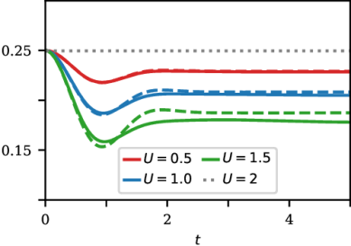
Figure 2: Double occupancy after a sudden quench. Continuous and dashed lines correspond, respectively, to DMFT and UPT computations for the disordered case in absence of long-range tails ($M_{\alpha}=0$) for different on-site interaction $U=0.5,1.0,1.5$ while the dotted line is a DMFT computation of the clean fully connected Fermi-Hubbard model ($\alpha=0$) at $U=2$. We observe the freezing of dynamics in absence of disorder and a relaxation to an equilibrium value, which decreases as $U$ increases, in the presence of it [34].

The absence of dynamical signatures after turning on the interaction can be justified analytically within the DMFT formalism for $\alpha<d$. The analytical derivation, fully reported in  can be summarized as follows: The core idea of DMFT is to simplify the many-body problem by approximating it with the problem of a single impurity coupled to a bath. Within the DMFT perspective, the single electron Green function looses its momentum dependence and depends only on the imaginary frequency $G(i\omega_{n})$. In order to obtain the impurity Green function one has to solve a self-consistent equation for the impurity self-energy $\Sigma(i\omega_{n})=\mathcal{G}_{0}^{-1}(i\omega_{n})-G^{-1}(i\omega_{n})$, where $\mathcal{G}_{0}(i\omega_{n})$ is the bare Green function of the local theory [24].

Due to the presence of the accumulation point in the DOS of the strong long-range system, the DMFT self-consistency condition for any $\alpha<d$ can be shown to converge to the bare Green function

$$\mathscr{G}^{-1}_{0}(i\omega_{n})=i\omega_{n}+\mu+\mathcal{O}(1/N),$$ (6)

which corresponds to the result in the atomic limit, i.e. in absence of kinetic energy ($\lim_{t_{r}\to 0}$). This is consistent with the flat-interacting $\alpha=0$ case where the kinetic and the interaction terms effectively commute in the thermodynamic limit [36] leading to the simultaneous conservation of the kinetic and potential energy. By turning on the local interactions a finite potential energy is suddenly imprinted onto the system but it cannot be dispersed in any way. Our derivation shows that this phenomenon is actually universal and occurs for any value of the power-law exponent $\alpha<1$ for the Hamiltonian in Eq. (1) in the thermodynamic limit .

In principle, one may expect DMFT to be not reliable in low dimension due to strong spatial fluctuations. However, strong long-range couplings are known to suppress spatial fluctuations [3], in analogy to what occurs to local couplings in infinite dimension, where mean-field approaches are known to become exact [38].

The disordered case: we argued that long-range interactions suppress spatial fluctuations, increasing the accuracy of mean-field approaches. At the same time, disorder ensures that momentum and energy conservation do not generate divergences in the unitary perturbation theory treatment of the problem. Thus, in both the DMFT and UPT study of the disordered case, turning on local interactions at $t>0$ only triggers scattering processes, which involve transitions among states within the continuous semi-circular portion of the spectrum for half-filled initial states and the dynamics are shielded from the low part of the spectrum.

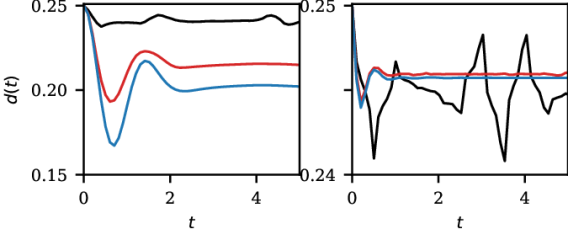
Figure 3: Double occupancy after a sudden quench to $U=1$ for $\alpha=0.5$ when $\sigma=1$ and $M_{0}=-4\pi$. In the left panel, the hopping has been re-escaled using Kac’s prescription while on the right one the hopping is un-scaled. Three different systems sizes are shown $L=2^{3},2^{6},2^{9}$ (black, red, blue line) from top to bottom close to $t=0$. For the smallest syze $L=2^{3}$ we observe the presence of Poincaré recurrences which already dephase both for $L=2^{6},2^{9}$

In presence of disorder, the continuous semicircular portion of the spectrum in Eq. (16) exactly corresponds to the DOS of the local system in the Bethe lattice. The addition of the long-range hopping amplitudes in Eq. (16) causes the appearance of a discrete set of low-energy quasi-particle states. However, these discrete states become statistically irrelevant in the thermodynamic limit washing away the effect of long-range interactions. This is readily shown by the self-consistent condition between the Weiss function and the local Green’s function which becomes $\mathscr{G}^{-1}_{0}(i\omega_{n})=i\omega_{n}+\mu-J^{2}G(i\omega_{n})+\mathcal{O}(1/N)$ for the DOS in Eq. (16).

We conclude that, in analogy with local quenches of the Ising model [17, 18], we shall also observe the effect of cooperative shielding in our case. The system does not feel the low energy states, and its dynamics, as well as the thermalization timescales, are solely determined by energies near the Fermi-surface. It is worth noting that the thermodynamic limit procedure is essential to obtain exact shielding of long-range interactions. Thus, in order to investigate the finite size signatures of shielding we employ the unitary perturbation theory (UPT) approach, which has already been successfully applied to the local case [39]. In UPT, the time evolution of an observable $\hat{A}$ can be computed by the expression

$$\braket{A}_{t}=\braket{A}_{0}+4U^{2}\int_{-\infty}^{\infty}d\omega\frac{\sin^{2}\left(\omega t/2\right)}{\omega^{2}}J(\omega)+\mathcal{O}(U^{3}),$$ (7)

where $J(\omega)=\braket{\hat{H}_{\text{int}}\left(\hat{A}-\braket{A}_{0}\right)\delta\left(\hat{H}_{0}-\braket{H_{0}}-\omega\right)\hat{H}_{\text{int}}}_{0}$ captures scattering processes up to second order in $U$.

In the local case $\alpha\to\infty$ UPT predicts a prethermalization plateau and the appearance of quasi-conserved charges, which lead to a generalized Gibbs distribution [26]. In Fig.3 (left panel) we present the results for the $\alpha=0.5$ case at half filling for different systems size $L=2^{3},2^{6},2^{9}$ both for scaled and unscaled hopping. By comparing the blue line on the bottom of Fig. 3 (left panel) with the blue dahsed line in the middle of Fig. 2, we observe how, as long as the system is considerably big, we recover the qualitative behavior of the infinite dimensional Bethe-Lattice [34] due to the cooperative shielding of long-range interactions. The dynamics stabilizes when the continuous part of the spectrum “equilibrates” by dephasing, while the signatures of the discrete states are shielded by the large size of the system.

On the other hand, at small sizes, the spectrum can be considered discrete everywhere and Poincaré revivals are observed. The presence or absence of the Kac’s renormalization factor only changes the magnitude on the change of the double occupancy without adding any temporal structure as we can see in Fig.3 (right panel). A justification of the magnitude change between the two cases comes from the scaling of $M_{0}\propto N^{(1-\alpha)}$ for the unscaled case. Due to this scaling, an extensive number of low-energy states lie outside the semi-circle reducing the spectral weight of the continuous semicircular part.

Fidelity: To support the universality of shielding and freezing, we analyze the fidelity between an initial state evolved under different Hamiltonians $H_{0}$ and $H_{\alpha}$ which correspond to Eq. (1) with $M_{\alpha}=0$ and $M_{\alpha}\neq 0$ respectively.

$$F(t)=\left|\bra{\Psi(0)}e^{it\hat{H}_{0}}e^{-it\hat{H}_{\alpha}}\ket{\Psi(0)}\right|^{2}.$$ (8)

Again, we perturb to second order in $U$. A naive comparison between two different realizations of the same Hamiltonian leads to a orthogonality catastrophe due to the random nature of the eigenstates . In order not lose the physics of the long-range in these details, we consider that the eigenvectors for both realizations are parallel and take into account their difference in the spectrum.

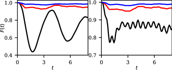
Figure 4: Fidelity decay when the system is evolved under purely random Gaussian hopping, $H_{0}$, vs one with hoppings sampled from Eq. (2) with $\alpha=0.5$, $H_{\alpha}$. In both cases $U=1$, $\sigma=1$ and $M_{0}=-2\pi$. The initial state corresponds to a filled Fermi-sea at half filling of the purely disorder case $H_{0}$. Three different systems sizes are shown $L=2^{3},2^{6},2^{9}$ and the panels correspond to different realizations of the disorder. The smallest system shows a dependence on the discrete low-energy states which is washed away as the system size increases.

In Fig.4 we plot the fidelity as a function of time for different system sizes and realizations of disorder. The shielding phenomenon manifest itself suppressing the dynamical fluctuations of the fidelity and proving, according to Eq. (47), that the presence of the low-energy discrete states generated by a finite $M_{\alpha}$ is inconsequential to the dynamics in the thermodynamic limit. At finite size, the periodic oscillations are a reminiscences of Poincaré recurrences coming from finite size effects but also comes from the perturbative nature of our calculation.

Conclusions and perspectives: We analyzed how long-range interacting systems thermalize using a Hubbard model with long-range hopping, driven out-of-equilibrium by a sudden quench of the local interaction. This quench caused an apparent localization of electrons and freezing of dynamics, similar to findings in Refs [18, 17]. For $\alpha<d$, low energy levels remain discrete in the thermodynamic limit, while high energy ones converge to a single point. Therefore, for large enough gaps, the occupations of these modes are fixed and are not affected by local interactions.. Consequently, a purely local Hamiltonian dominates within a subspace of excited states, applicable for a limited time frame.

The re-scaling of hopping amplitudes, using the Kac factor, ensures finite spectral gaps but makes kinetic energy sub-extensive, leaving overall dynamics dictated by the potential term. Without this re-scaling, energy levels are infinitely gapped in the thermodynamic limit, prohibiting transitions and the interaction only mixes the accumulated high energy modes, leading to the freezing phenomenon.

In the presence of disorder, the low-energy spectrum remains discrete, while the accumulation point forms a continuous semi-circular density of states (DOS). At half-filling, the Fermi surface lies within these continuum modes, where most dynamics occur. Using unitary perturbation theory, we observed that the system’s evolution mirrors that of a local system on an infinite-dimensional Bethe lattice, leading to the complete shielding of long-range interactions in the thermodynamic and to subsequent equilibration..

Our study shows that several out-of-equilibrium properties of long-range couplings are linked to the quasi-particle spectrum, observable across various degrees of freedom (e.g., spin or particles), quasi-particle statistics (Fermi or Bose), quench types (local or global), and values of $\alpha$. Future studies shall clarify how the quasi-particle picture links to the many-body spectrum [21] or to the Vlasov description of long-range systems [41], paving the way to the understanding of the undergoing cavity experiments [11].

Acknowledgements This research was supported in part by grant NSF PHY-1748958 to the Kavli Institute for Theoretical Physics (KITP). This research was funded by the Swiss National Science Foundation (SNSF) grant number 200021 207537, by the Deutsche Forschungsgemeinschaft (DFG, German Research Foundation) under Germany’s Excellence Strategy EXC2181/1-390900948 (the Heidelberg STRUCTURES Excellence Cluster) and the Swiss State Secretariat for Education, Research and Innovation (SERI).

I Supplementary Material

II Spectrum of Gaussian Random Matrix.

The eigenvalue spectrum of a real symmetric $N\times N$ matrix $\mathbf{M}$ with eigenvalues $M_{\lambda}$ is,

$$\nu(\lambda)=\frac{1}{N}\sum_{\lambda}\delta(\lambda-M_{\lambda}).$$ (9)

Which can be redefined by analytically continuing $\lambda$ such that it contains a negative imaginary part $-i\epsilon$ to obtain,

$$\nu(\lambda)=\frac{1}{\pi N}\text{Im}\left(\nu-i\epsilon-M_{\lambda})\right)^{-1}$$ (10)

using

$$\text{det}\left(1\kern-2.5pt\text{l}\lambda-\mathbf{M}\right)=\prod_{\lambda}\left(\lambda-M_{\lambda}\right)$$ (11)

we can rewrite Eq. (16) as

$$\nu(\lambda)=\frac{1}{N\pi}\text{Im}\frac{\partial}{\partial\lambda}\ln\left(\text{det}\left(1\kern-2.5pt\text{l}(\lambda-i\epsilon)-\mathbf{M}\right)\right).$$ (12)

The logarithm can be rewritten using the following trick

$$\ln(x)=\lim_{n\rightarrow 0}\frac{x^{n}-1}{n},$$ (13)

and by plugging this back into Eq. (12) we get

$$\nu(\lambda)=\frac{-2}{N\pi}\text{Im}\frac{\partial}{\partial\lambda}\lim_{n\rightarrow 0}\frac{1}{n}\left(\text{det}^{-1/2}\left(1\kern-2.5pt\text{l}(\lambda-i\epsilon)-\mathbf{M}\right)^{n}-1\right).$$ (14)

For later convenience, we will express the determinant as a Gaussian integral

$$\text{det}^{-1/2}\left(1\kern-2.5pt\text{l}\lambda-\mathbf{M}\right)=\left(\frac{e^{i\pi/4}}{\pi^{1/2}}\right)^{N}\int_{-\infty}^{\infty}\prod_{i}dx_{i}\exp\left(-i\sum_{ij=1}^{N}x_{i}\left(\delta_{ij}\lambda-M_{ij}\right)x_{j}\right),$$ (15)

where the imaginary part of $\lambda$ has been reabsorbed into the definition of $\lambda$ itself and it is needed to ensure convergence. We then obtain the basic result from [32].

$$\nu(\lambda)=\frac{2}{N\pi}\text{Im}\frac{\partial}{\partial\lambda}\lim_{n\rightarrow 0}\frac{1}{n}\left(\left(\frac{e^{i\pi/4}}{\pi^{1/2}}\right)^{nN}\int_{-\infty}^{\infty}\prod_{i}dx_{i}\exp\left(-i\sum_{ij:\beta}^{N}x^{\beta}_{i}\left(\delta_{ij}\lambda-M_{ij}\right)x^{\beta}_{j}\right)-1\right).$$ (16)

Where the integration now runs over $Nn$ variables $x^{\beta}_{i}$.

II.1 Long-range mean values.

Now, we will allow each value $M_{ij}$ to fluctuate around a mean-value which will depend on $i,j$, $M_{0}(|i-j|)$, such that the probability distribution of $M_{ij}$i s given by

$$P[M_{ij}]=\frac{1}{\sqrt{2\pi\sigma^{2}}}\exp\left(-\frac{\left(M_{ij}-M_{0}(|i-j|)\right)^{2}}{2\sigma^{2}}\right),\hskip 28.45274ptM_{0}(|i-j|)=\frac{M_{\alpha}}{\left|i-j\right|^{\alpha}}.$$ (17)

This would correspond to a disordered model which, in average, behaves in a long-range manner.

By ensemble averaging Eq. (16) over all configurations $M_{ij}$ we obtain the average density of state $\rho(\lambda)$

$$\rho(\lambda)=\int\prod dM_{ij}P[M_{ij}]\nu\left(\lambda;\{M_{ij}\}\right).$$ (18)

For the Guassian probabily densities of Eq. (17) we can carry out the integration over the ensemble

$$\begin{split}\rho(\nu)=\frac{-2}{\pi N}\text{Im}\frac{\partial}{\partial\lambda}\lim_{n\rightarrow 0}\frac{1}{n}\Bigg{(}&\left(\frac{e^{i\pi/4}}{\pi^{1/2}}\right)^{Nn}\int_{-\infty}^{\infty}\prod dx_{i}\exp\left(-i\sum_{ij,\beta}x^{\beta}_{i}\left(\lambda\delta_{ij}-\frac{M_{\alpha}}{|i-j|^{\alpha}}\right)x^{\beta}_{j}\right)\\ &\exp\left(-\sigma^{2}\sum_{i,j}\left(\sum_{\beta}x^{\beta}_{i}x^{\beta}_{j}\right)^{2}\right)\exp\left(\sigma^{2}\sum_{i}\left(\sum_{\beta}\left(x^{\beta}_{i}\right)^{2}\right)^{2}\right)-1\Bigg{)}\end{split}$$ (19)

Ultimately, we are interesting in the limit of $N\rightarrow\infty$ so we should look for leading order in $N$ and at most linear in $n$. Taking this into account, looking back at the exponential in Eq. (21) we can cancel terms of second order in $n$,

$$\frac{J^{2}}{N}\sum_{ij}\left(\sum_{\beta}x^{\beta}_{i}x^{\beta}_{j}\right)^{2}=\frac{J^{2}}{N}\sum_{\beta}\left(\sum_{i}\left(x^{\beta}_{i}\right)^{2}\right)^{2}+\frac{J^{2}}{N}\sum_{\gamma\neq\beta}x^{\gamma}_{i}x^{\gamma}_{j}x^{\beta}_{i}x^{\beta}_{j},$$ (20)

doing so, we will only need to retain the first term in Eq. (20) where $\alpha=\beta$.

$$\begin{split}\rho(\nu)=\frac{-2}{\pi N}\text{Im}\frac{\partial}{\partial\lambda}\lim_{n\rightarrow 0}\frac{1}{n}\Bigg{(}\left(\frac{e^{i\pi/4}}{\pi^{1/2}}\right)^{Nn}\int_{-\infty}^{\infty}\prod dx_{i}\exp\left(-i\sum_{ij}x_{i}\left(\lambda\delta_{ij}-\frac{M_{\alpha}}{|i-j|^{\alpha}}\right)x_{j}-\frac{J^{2}}{N}\left(\sum_{i}x^{2}_{i}\right)^{2}\right)^{n}\\ -1\Bigg{)}.\end{split}$$ (21)

By introducing an auxiliary field $s$, we can parametrize the second exponential in the integral above as

$$\exp\left(-\frac{J^{2}}{N}\left(\sum_{i}x^{2}_{i}\right)^{2}\right)=\left(\frac{N}{2\pi}\right)^{1/2}\frac{\lambda}{\left(2J^{2}\right)^{1/2}}\int_{-\infty}^{\infty}ds\exp\left(-\frac{\lambda^{2}}{4J^{2}}Ns^{2}-i\lambda s\sum_{i}x_{i}^{2}\right),$$ (22)

and with this the integral from Eq. (21) simplifies to

$$\begin{split}\rho(\nu)=\frac{-2}{\pi N}\text{Im}\frac{\partial}{\partial\lambda}\lim_{n\rightarrow 0}\frac{1}{n}\Bigg{(}&\left(\frac{e^{i\pi/4}}{\pi^{1/2}}\right)^{Nn}\left(\frac{N}{2\pi}\right)^{n/2}\frac{\lambda^{n}}{\left(2J^{2}\right)^{n/2}}\\ &\int_{-\infty}^{\infty}ds\int_{-\infty}^{\infty}\prod dx_{i}\exp\left(-i\sum_{ij}x_{i}\left(\lambda(1+s)\delta_{ij}-\frac{M_{\alpha}}{|i-j|^{\alpha}}\right)x_{j}-\frac{\lambda^{2}}{4J^{2}}Ns^{2}\right)^{n}-1\Bigg{)}\end{split}$$ (23)

By looking at the case of particles with long-range hopping as in [22], we know that a unitary transformation $U$ exist that diagonalizes the matrix with entries $M_{ij}=\lambda(1+s)\delta_{ij}-M_{\alpha}/|i-j|^{\alpha}$. It is convenient to rewrite Eq. (23) in such basis

$$\begin{split}\rho(\nu)=\frac{-2}{\pi N}\text{Im}\frac{\partial}{\partial\lambda}\lim_{n\rightarrow 0}\frac{1}{n}\Bigg{(}&\left(\frac{e^{i\pi/4}}{\pi^{1/2}}\right)^{Nn}\left(\frac{N}{2\pi}\right)^{n/2}\frac{\lambda^{n}}{\left(2J^{2}\right)^{n/2}}\\ &\int_{-\infty}^{\infty}ds\int_{-\infty}^{\infty}\prod_{k}db_{k}\exp\left(-i\sum_{k}b_{k}\left(\lambda(1+s)-M_{\alpha}\epsilon_{k}\right)b_{k}-\frac{\lambda^{2}}{4J^{2}}Ns^{2}\right)^{n}-1\Bigg{)},\end{split}$$ (24)

where now $\epsilon_{k}$ is the dispersion relation of a tight-binding model with long-range hopping parameters as in [22].

$$\epsilon_{k}=M_{\alpha}\frac{\text{Re}\left[\text{Li}\left(e^{ik}\right)\right]}{2},\hskip 14.22636pt\hskip 28.45274pt\epsilon_{k}=M_{\alpha}N^{1-\alpha}\int_{0}^{1/2}\frac{\cos\left(2\pi ns\right)}{s^{\alpha}}\hskip 14.22636ptk=\frac{2\pi n}{N}\hskip 14.22636pt-\frac{N}{2}<n\leq\frac{N}{2}$$ (25)

The integral over the $b_{k}$ variables can be evaluated by noticing that the

$$\begin{split}\rho(\nu)=\frac{-2}{\pi N}\text{Im}\frac{\partial}{\partial\lambda}\lim_{n\rightarrow 0}\frac{1}{n}\Bigg{(}&\Bigg{[}\left(\frac{e^{i\pi/4}}{\pi^{1/2}}\right)^{N}\left(\frac{N}{2\pi}\right)^{1/2}\left(\frac{\pi^{N}}{2J^{2}}\right)^{1/2}\lambda\exp\left(-\frac{N}{2}\ln\lambda\right)\\ &\int_{-\infty}^{\infty}ds\exp\left(-Ng(s)\right)\prod_{k}\left(\frac{1+s}{i(s_{k}-s)}\right)^{1/2}\Bigg{]}^{n}-1\Bigg{)}\end{split}$$ (26)

where

$$g(s)=\frac{\lambda^{2}s^{2}}{4J^{2}}+\frac{1}{2}\ln\left(i(1+s)\right)\hskip 28.45274pts_{k}\equiv-1+\frac{M_{\alpha}\epsilon_{k}}{\lambda}$$ (27)

In the limit of $N\rightarrow\infty$ can evaluate the integral in Eq. (26) by using a saddle-point approximation due to exponential factor, we just have to take special care close to each $s_{k}$. As pointed out in [32], the saddle point approximation is responsible for the semicircular density of states for $|\lambda|<2J^{2}$. A Taylor expansion of $g(s)$ around $s_{k}$ gives

$$g(s)\approx g(s_{k})+\frac{\lambda}{2J^{2}}(\lambda_{k}-\lambda)(s-s_{k})+\frac{\lambda^{2}}{4}\left(\frac{1}{J^{2}}-\frac{1}{M_{\alpha}^{2}\epsilon_{k}^{2}}\right)(s-s_{k})^{2}+...$$ (28)

with

$$\lambda_{k}=M_{\alpha}\epsilon_{k}+\frac{J^{2}}{M_{\alpha}\epsilon_{k}}$$ (29)

therefore, when $\lambda=\lambda_{n}$, $g(s)$ has a turning point. One can also see that for for $M_{0}\epsilon_{n}^{2}>J$ this turning point is a minimum, while it is a maximum for $M_{0}\epsilon_{n}^{2}<J$. Moreover this turning points lie outside of the semicircular continuum of eigenvalues. The integral in Eq. (26) is evaluated by retaining the first two terms of the Taylor expansion of $g(s)$. The result is

$$\begin{split}\rho(\nu)=\frac{-2}{\pi N}\text{Im}\frac{\partial}{\partial\lambda}\lim_{n\rightarrow 0}\frac{1}{n}\Bigg{(}&\Bigg{[}\left(\frac{e^{i\pi/4}}{\pi^{1/2}}\right)^{N}\left(\frac{N}{2\pi}\right)^{1/2}\left(\frac{\pi^{N}}{2J^{2}}\right)^{1/2}\exp\left(-\frac{N}{2}\ln\lambda\right)\\ &\hskip 56.9055pt\exp\left(-Ng(s_{k})\right)\exp\left(-\frac{1}{2}\ln\left(\lambda-\lambda_{k}\right)\right)\Bigg{]}^{n}-1\Bigg{)}\end{split}$$ (30)

with

$$g(s_{k})=-\frac{\lambda^{2}}{4J^{2}}\left(\frac{M_{\alpha}\epsilon_{k}}{\lambda}-1\right)^{2}+\frac{\ln\lambda}{2}-\frac{\ln M_{\alpha}\epsilon_{k}}{2}-\frac{i\pi}{4}$$ (31)

Plugging this back into Eq. (21) and using Eq. (13) the eigenvalue spectrum for $M_{\alpha}\epsilon_{k}>J$ is

$$\rho(\lambda)=-\frac{2}{N\pi}\text{Im}\frac{\partial}{\partial\lambda}\left[-\frac{1}{2}\ln\left(\lambda-\lambda_{k}\right)\right]=\frac{1}{N}\delta(\lambda-\lambda_{k})$$ (32)

The eigenvalue spectrum of a large random symmetric matrix where the mean value has a power-law dependence with the distance from the diagonal is

$$\rho(\lambda)=\frac{\sqrt{4J^{2}-\lambda^{2}}}{2\pi J^{2}}+\frac{1}{N}\sum_{k\forall k\in\epsilon_{k}<\epsilon^{*}}\delta(\lambda-\lambda_{k})\hskip 14.22636pt\text{where}\hskip 14.22636pt\epsilon^{*}\equiv\frac{J}{M_{\alpha}}.$$ (33)

We would like to point out that this computation assumes that we can analyze $g(s)$ in the neighborhood of each $s_{k}$ independently, which is valid when our energy levels $e_{k}$ are gaped. Due to this fact we can only predict correctly the density of states of strongly interacting systems $\alpha<d$ where we know the spectrum remains gaped in the thermodynamic limit.

III Dynamical Mean-Field Theory.

Dynamical mean-field theory replaces a lattice many-body problem to a single-site quantum impurity one. By doing so, one does not consider spatial fluctuations but only keeps track of temporal ones. For a Hubbard model with on site interactions the impurity effective dynamics are described by the imaginary-time action

$$S_{\text{eff}}=-\int_{0}^{\beta}d\tau\int_{0}^{\beta}d\tau^{\prime}\sum_{\sigma}c^{\dagger}_{0,\sigma}(\tau)\mathscr{G}^{-1}_{0}(\tau-\tau^{\prime})c_{0\sigma}(\tau^{\prime})-iU\int_{0}^{\beta}d\tau n_{0\uparrow}(\tau)n_{0\downarrow}(\tau)$$ (34)

where $(c_{0\sigma},c^{\dagger}_{0\sigma})$ are the fermionic degrees of freedom of the impurity.

Within DMFT the self-consistent equation that determines the relation of the effective single site Green’s function and the on-site lattice interacting Green’s function is given by

$$\mathscr{G}^{-1}_{0}(i\omega_{n})=i\omega_{n}+\mu+G^{-1}(i\omega_{n})-R[G],$$ (35)

where $R[G]$ is the reciprocal function defined as

$$\tilde{\rho}(\xi)\equiv\int d\varepsilon\frac{\rho(\varepsilon)}{\xi-\varepsilon},\hskip 28.45274ptR[\tilde{\rho}(\xi)]=\xi.$$ (36)

In general, one cannot find an explicit connection between $\mathscr{G}^{-1}_{0}(i\omega_{n})$ and $G(i\omega_{n})$.

III.1 Long-range hopping.

As a pedagogical example we will look at the case where the particles are allowed to hop everywhere in the lattice. The density of states of such systems consist of an isolated eigenvalue plus an accumulation point at zero energy

$$\rho(\varepsilon)=\frac{1}{N}\delta(\varepsilon-\varepsilon_{0})+\frac{N-1}{N}\delta(\varepsilon)$$ (37)

for such DOS after computing the reciprocal function Eq.36, the self-consistent relation between the Weiss field and the local Green’s function reads as

$$\mathscr{G}^{-1}_{0}(i\omega_{n})=i\omega_{n}+\mu+G^{-1}(i\omega_{n})-\frac{\left(N+\varepsilon_{0}+\varepsilon_{0}NG(i\omega_{n})\right)-\left(\left(\varepsilon_{0}-N+\varepsilon_{0}NG(i\omega_{n})\right)^{2}+4\varepsilon_{0}N\right)^{1/2}}{2NG(i\omega_{n})},$$ (38)

which, on the limit of $N\rightarrow\infty$ becomes

$$\mathscr{G}^{-1}_{0}(i\omega_{n})=i\omega_{n}+\mu-\frac{1}{N}\frac{\varepsilon_{0}}{\varepsilon_{0}G(i\omega_{n})-1}=i\omega_{n}+\mu-\mathcal{O}(1/N).$$ (39)

In the limit of larger $N$ one recovers the atomic limit where all sites are disconnected and particles cannot hop in between them.

The situation changes slightly when the hopping are not rescaled under Kac’s prescription. Substituing $\varepsilon_{0}\equiv N\varepsilon_{0}$ and expanding Eq.38

$$\mathscr{G}^{-1}_{0}(i\omega_{n})=i\omega_{n}+\mu-\frac{1}{4N}\frac{\left(\varepsilon_{0}+1\right)^{2}}{\varepsilon_{0}G^{2}(i\omega_{n})}=i\omega_{n}+\mu-\mathcal{O}(1/N).$$ (40)

III.2 Semi-circular density of states.

For the case of a semi-circular density of states of the form,

$$\rho(\varepsilon)=\frac{1}{2\pi J^{2}}\sqrt{4J^{2}-\varepsilon^{2}}$$ (41)

one obtains

$$\tilde{\rho}(\xi)=\frac{\xi-\sqrt{\xi^{2}-4J^{2}}}{2J^{2}},\hskip 28.45274ptR[\tilde{\rho}(G)]=J^{2}G+\frac{1}{G}.$$ (42)

which leads an explicit form between the local Green’s function and the effective Weiss field

$$\mathscr{G}^{-1}_{0}(i\omega_{n})=i\omega_{n}+\mu-J^{2}G(i\omega_{n}).$$ (43)

For our long-range interacting systems with disorder, we have seen how the density of states consist of a finite set of discrete energy levels $\varepsilon_{n}\in$ on top of a semi-circular continuum. This leads to the following Hilbert transform,

$$\tilde{D}(\xi)=\frac{1}{N}\frac{\xi-\sqrt{\xi^{2}-4J^{2}}}{2J^{2}}+\sum_{\varepsilon_{n}\in{\varepsilon*}}\frac{1}{N}\frac{1}{\xi-\varepsilon_{n}},$$ (44)

an explicit expression for the reciprocral function cannot be found but it is easy to see that on the limit of $N\rightarrow\infty$ the set of discrete points, with a factor of $1/N$ in front, can be thought as a correction tot the general semi-circular form,

$$\mathscr{G}^{-1}_{0}(i\omega_{n})=i\omega_{n}+\mu-t^{2}G(i\omega_{n})+\mathcal{O}(1/N).$$ (45)

IV Fidelity computation.

The fidelity consist on the overlap between the same state evolved under different Hamiltonians. In the case of our interest, we would like to compare our random hopping Hamiltonian with long-range tails to one where the hoping amplitudes are sampled from a Gaussian distribution zero mean.

$$\begin{split}&\hat{H}_{0}=\sum_{ij}t_{ij}\left(\hat{c}^{\dagger}_{i,\uparrow}\hat{c}_{j,\uparrow}+\hat{c}^{\dagger}_{i,\downarrow}\hat{c}_{j,\downarrow}\right)+U\sum_{i}\hat{c}^{\dagger}_{i,\uparrow}\hat{c}_{i,\uparrow}\hat{c}^{\dagger}_{i,\downarrow}\hat{c}_{i,\downarrow},\\ &\hat{H}_{\alpha}=\sum_{ij}M_{ij}\left(\hat{c}^{\dagger}_{i,\uparrow}\hat{c}_{j,\uparrow}+\hat{c}^{\dagger}_{i,\downarrow}\hat{c}_{j,\downarrow}\right)+U\sum_{i}\hat{c}^{\dagger}_{i,\uparrow}\hat{c}_{i,\uparrow}\hat{c}^{\dagger}_{i,\downarrow}\hat{c}_{i,\downarrow}.\end{split}$$ (46)

As an initial state we take the ground state of the kinetic term in $H_{0}$ at half-filling, which we denote as $\ket{F.S.}$.

$$F(t)=\left|\bra{\text{F.S.}}e^{it\hat{H}_{0}}e^{-it\hat{H}_{\alpha}}\ket{\text{F.S.}}\right|^{2}.$$ (47)

In order to be able to capture correctly the physics behind the long-range nature of the tails such that they are not washed away by the randomness of the system a few assumptions are in order. Since the eigenvectors of a Guassian $L\times L$ orthogonal matrix are random unit vectors on the surface of a $L$ dimensional sphere, a naive computation of the fidelity for two different realizations of disorder would quickly tend to zero due to a orthogonality catastrophe effect. We will, therefore, assume that the eigenvectors between both realizations are the same and that only their eigen-energies change in the presence of long-range tails.

Both Hamiltonians in Eq.46 can be rewritten in terms of the random vectors that diagonalize the hoping term as,

$$\begin{split}\hat{H}_{0}=\sum_{l}\varepsilon_{n}\left(\hat{b}^{\dagger}_{n,\uparrow}\hat{b}_{n,\uparrow}+\hat{b}^{\dagger}_{n,\downarrow}\hat{b}_{n,\downarrow}\right)+U\sum_{i}\sum_{l_{1},l_{2},l_{3},l_{4}}a^{*}_{i,l_{1}}a_{i,l_{2}}a^{*}_{i,l_{3}}a_{i,l_{4}}\hat{b}^{\dagger}_{l_{1},\uparrow}\hat{b}_{l_{2},\uparrow}\hat{b}^{\dagger}_{l_{3},\downarrow}\hat{b}_{l_{4},\downarrow},\\ \hat{H}_{\alpha}=\sum_{l}\varepsilon^{\prime}_{n}\left(\hat{b}^{\dagger}_{n,\uparrow}\hat{b}_{n,\uparrow}+\hat{b}^{\dagger}_{n,\downarrow}\hat{b}_{n,\downarrow}\right)+U\sum_{i}\sum_{l_{1},l_{2},l_{3},l_{4}}a^{*}_{i,l_{1}}a_{i,l_{2}}a^{*}_{i,l_{3}}a_{i,l_{4}}\hat{b}^{\dagger}_{l_{1},\uparrow}\hat{b}_{l_{2},\uparrow}\hat{b}^{\dagger}_{l_{3},\downarrow}\hat{b}_{l_{4},\downarrow}.\end{split}$$ (48)

The coefficients $a_{i,l}$ are random numbers restricted to fulfill $\sum_{l}|a_{i,l}|^{2}=1$ and $\varepsilon_{n}$,$\varepsilon^{\prime}_{n}$ differ only in the finite subset of energy levels $n$ that lie outside the semicircular.

Again, the interacting term is treated as a small perturbation and expanded up to second order using unitary perturbation theory. We start with a Hamiltonian of the form $\hat{H}=\hat{H}_{0}+g\hat{H}_{1}$ and tranform it via a canonical transformation $e^{\hat{S}}$ chosen to cancel, at each order of $g$, every off-diagonal term.

$$\begin{split}&\hat{S}=g\hat{S}_{1}+\frac{1}{2}g^{2}\hat{S}_{2}+\mathcal{O}(g^{3}),\\ &\hat{H}_{\text{diag}}=e^{\hat{S}}\hat{H}e^{-\hat{S}}=H_{0}+g\left(\hat{H}_{1}+[\hat{S}_{1},\hat{H}_{0}]\right)+g^{2}\left(\frac{1}{2}[\hat{S}_{2},\hat{H}_{0}]+[\hat{S}_{1},\hat{H}_{1}]+\frac{1}{2}[\hat{S}_{1},[\hat{S}_{1},\hat{H}_{0}]]\right)+\mathcal{O}(g^{3})\end{split}$$ (49)

the transformed Hamiltonian and the unitary transformation read

$$\begin{split}\hat{H}_{\text{diag}}&=e^{\hat{S}}\hat{H}e^{-\hat{S}}=\hat{H}_{0}+g\hat{H}_{\text{diag}}^{(1)}+g^{2}\hat{H}_{\text{diag}}^{(2)}+O(g^{3}),\\ \bra{n}\hat{S}_{1}\ket{m}&=\begin{cases}\bra{n}\hat{H}_{1}\ket{m}&\text{if }n\neq m\\ 0&\text{if }n=m\end{cases},\\ \bra{n}\hat{S}_{2}\ket{m}&=\begin{cases}\bra{n}[\hat{S}_{1},\hat{H}_{1}+\hat{H}_{\text{diag}}^{(1)}]\ket{m}&\text{if }n\neq m\\ 0&\text{if }n=m\end{cases},\\ \hat{H}_{\text{diag}}^{(i)}&=\sum_{n}\ket{n}E^{(i)}_{n}\bra{n},\\ E^{(1)}_{n}&=\bra{n}\hat{H}_{1}\ket{n},\quad E^{(2)}_{n}=\sum_{m\neq n}\frac{|\bra{n}\hat{H}_{1}\ket{m}|^{2}}{E_{n}-E_{m}}\end{split}$$ (50)

the operator $\hat{S}$ which transforms the Hamiltonian $H_{0}$ is, to first order

$$S=U\sum_{i}\sum^{\prime}_{l_{1},l_{2},l_{3},l_{4}}\frac{a^{*}_{i,l_{1}}a_{i,l_{2}}a^{*}_{i,l_{3}}a_{i,l_{4}}}{\varepsilon_{l_{1}}-\varepsilon_{l_{2}}+\varepsilon_{l_{3}}-\varepsilon_{l_{4}}}\hat{b}^{\dagger}_{l_{1},\uparrow}\hat{b}_{l_{2},\uparrow}\hat{b}^{\dagger}_{l_{3},\downarrow}\hat{b}_{l_{4},\downarrow}$$ (51)

where the $\sum^{\prime}$ denotes that the term $l_{1}=l_{2}\land l_{3}=l_{4}$ is excluded. It is straightforward to see that the $S^{\prime}$ which transform $H_{\alpha}$ has the same form as $S$ but with the substitution of $\varepsilon_{i}\rightarrow\varepsilon^{\prime}_{i}$.

With this, we can go back to Eq.47 and express it in terms of $S$ and $S^{\prime}$.

$$F(t)=\left|\bra{\text{F.S.}}_{0}e^{S(0,0)-S(0,-t)}e^{S^{\prime}(-t,0)-S^{\prime}(0,0)}\ket{\text{F.S.}}_{0}\right|^{2}$$ (52)

where we have defined $S(-t,0)=e^{-it\hat{H}_{0\text{diag}}}Se^{it\hat{H}_{0\text{diag}}}$ and $S(0,-t)=e^{-it\hat{H}_{\alpha\text{diag}}}Se^{it\hat{H}_{\alpha\text{diag}}}$ and already canceled any phase factors given by the evaluation of diagonal terms $e^{-it\hat{H}_{\alpha\text{diag}}}\ket{F.S.}$ since the fidelity is defined as the modulus of the overlap.

We then expand the exponentials up to second order and evaluate to obtain

$$\begin{split}F(t)=&1-8U^{2}\sum_{ij}\sum_{\begin{subarray}{c}l_{1},l_{2}\\ l_{3}\neq l_{3}\end{subarray}}|a_{i,l_{1}}|^{2}|a_{j,l_{2}}|^{2}a^{*}_{i,l_{3}}a_{j,l_{3}}a^{*}_{j,l_{4}}a_{i,l_{4}}\left(n_{l_{1}}-\delta_{l_{1},l_{3}}(n_{l_{1}}-1))n_{l_{3}}n_{l_{3}}(1-n_{l_{4}})\right)\\ &\hskip 28.45274pt\times\Bigg{[}\frac{\sin^{2}\left(\left(\varepsilon_{l_{3}}-\varepsilon_{l_{4}}\right)/2\right)}{\left(\varepsilon_{l_{3}}-\varepsilon_{l_{4}}\right)^{2}}+\frac{\sin^{2}\left(\left(\varepsilon^{\prime}_{l_{3}}-\varepsilon^{\prime}_{l_{4}}\right)/2\right)}{\left(\varepsilon^{\prime}_{l_{3}}-\varepsilon^{\prime}_{l_{4}}\right)^{2}}\\ &\hskip 56.9055pt-2\cos\left(\frac{\varepsilon_{l_{3}}-\varepsilon_{l_{4}}-\varepsilon^{\prime}_{l_{3}}+\varepsilon^{\prime}_{l_{4}}}{2}\right)\frac{\sin\left(\left(\varepsilon_{l_{3}}-\varepsilon_{l_{4}}\right)/2\right)\sin\left(\left(\varepsilon^{\prime}_{l_{3}}-\varepsilon^{\prime}_{l_{4}}\right)/2\right)}{\left(\varepsilon_{l_{3}}-\varepsilon_{l_{4}}\right)\left(\varepsilon_{l^{\prime}_{3}}-\varepsilon_{l^{\prime}_{4}}\right)}\Bigg{]}\\ &-U^{2}\sum_{ij}\sum_{\begin{subarray}{c}l_{1}\neq l^{\prime}_{1}l_{3}\neq l^{\prime}_{3}\end{subarray}}a^{*}_{i,l_{1}}a_{j,l_{1}}a^{*}_{j,l^{\prime}_{1}}a_{i,l^{\prime}_{1}}a^{*}_{i,l_{3}}a_{j,l_{3}}a^{*}_{j,l_{0}}a_{i,l_{0}}\left(n_{l_{1}}n_{l_{3}}(1-n_{l^{\prime}_{1}})(1-n_{l_{0}})\right)\\ &\hskip 28.45274pt\times\Bigg{[}\frac{\sin^{2}\left(\left(\varepsilon_{l_{1}}-\varepsilon_{l_{2}}+\varepsilon_{l_{3}}-\varepsilon_{l_{4}}\right)/2\right)}{\left(\varepsilon_{l_{1}}-\varepsilon_{l_{2}}+\varepsilon_{l_{3}}-\varepsilon_{l_{4}}\right)^{2}}+\frac{\sin^{2}\left(\left(\varepsilon^{\prime}_{l_{1}}-\varepsilon^{\prime}_{l_{2}}+\varepsilon^{\prime}_{l_{3}}-\varepsilon^{\prime}_{l_{4}}\right)/2\right)}{\left(\varepsilon^{\prime}_{l_{1}}-\varepsilon^{\prime}_{l_{2}}+\varepsilon^{\prime}_{l_{3}}-\varepsilon^{\prime}_{l_{4}}\right)^{2}}\\ &\hskip 56.9055pt-2\cos\left(\frac{\varepsilon_{l_{1}}-\varepsilon_{l_{2}}+\varepsilon_{l_{3}}-\varepsilon_{l_{4}}-\varepsilon^{\prime}_{l_{1}}+\varepsilon^{\prime}_{l_{2}}-\varepsilon^{\prime}_{l_{3}}+\varepsilon_{l_{4}}}{2}\right)\\ &\hskip 113.81102pt\times\frac{\sin\left(\left(\varepsilon_{l_{1}}-\varepsilon_{l_{2}}+\varepsilon_{l_{3}}-\varepsilon_{l_{4}}\right)/2\right)\sin\left(\left(\varepsilon^{\prime}_{l_{1}}-\varepsilon^{\prime}_{l_{2}}+\varepsilon^{\prime}_{l_{3}}-\varepsilon^{\prime}_{l_{4}}\right)/2\right)}{\left(\varepsilon_{l_{1}}-\varepsilon_{l_{2}}+\varepsilon_{l_{3}}-\varepsilon_{l_{4}}\right)\left(\varepsilon_{l^{\prime}_{1}}-\varepsilon_{l^{\prime}_{2}}+\varepsilon_{l^{\prime}_{3}}-\varepsilon_{l^{\prime}_{4}}\right)}\Bigg{]}.\end{split}$$ (53)

As a last step we substitute the sum over the sites $\{i,j\}$ by averages over disorder. To do so notice that $a_{i,l}$ are components of a random unit vectors and perform the average by using the following probability distribution,

$$P[|a_{i,j}|^{2}]=\frac{\Gamma\left(\frac{L}{2}\right)}{\sqrt{\pi}\Gamma\left(\frac{l-1}{2}\right)}\frac{\left(1-|a_{i,j}|^{2}\right)^{(L-3)/2}}{|a_{i,j}|},\hskip 28.45274pt\lim_{L\rightarrow\infty}P[z=y/L]=\frac{e^{-z/2}}{\sqrt{2\pi z}}$$ (54)

References

- Polkovnikov et al. [2011] A. Polkovnikov, K. Sengupta, A. Silva, and M. Vengalattore, Rev. Mod. Phys. 83, 863 (2011).
- Srednicki [1994] M. Srednicki, Phys. Rev. E 50, 888 (1994).
- Defenu et al. [2023a] N. Defenu, T. Donner, T. Macrì, G. Pagano, S. Ruffo, and A. Trombettoni, Rev. Mod. Phys. 95, 035002 (2023a).
- Defenu et al. [2023b] N. Defenu, A. Lerose, and S. Pappalardi, (2023b), arXiv:2307.04802 [cond-mat.quant-gas] .
- Saffman et al. [2010] M. Saffman, T. G. Walker, and K. Mølmer, Rev. Mod. Phys. 82, 2313 (2010).
- Chomaz et al. [2022] L. Chomaz, I. Ferrier-Barbut, F. Ferlaino, B. Laburthe-Tolra, B. L. Lev, and T. Pfau, Reports on Progress in Physics 86, 026401 (2022).
- Carr et al. [2009] L. D. Carr, D. DeMille, R. V. Krems, and J. Ye, New Journal of Physics 11, 055049 (2009).
- Monroe et al. [2021] C. Monroe, W. C. Campbell, L.-M. Duan, Z.-X. Gong, A. V. Gorshkov, P. W. Hess, R. Islam, K. Kim, N. M. Linke, G. Pagano, P. Richerme, C. Senko, and N. Y. Yao, Rev. Mod. Phys. 93, 025001 (2021).
- Ritsch et al. [2013] H. Ritsch, P. Domokos, F. Brennecke, and T. Esslinger, Rev. Mod. Phys. 85, 553 (2013).
- Farokh Mivehvar and Ritsch [2021] T. D. Farokh Mivehvar, Francesco Piazza and H. Ritsch, Advances in Physics 70, 1 (2021), https://doi.org/10.1080/00018732.2021.1969727 .
- Wu et al. [2023a] Z. Wu, J. Fan, X. Zhang, J. Qi, and H. Wu, Phys. Rev. Lett. 131, 243401 (2023a).
- Ladd et al. [2010] T. D. Ladd, F. Jelezko, R. Laflamme, Y. Nakamura, C. Monroe, and J. L. O’Brien, Nature (London) 464, 45 (2010), arXiv:1009.2267 [quant-ph] .
- Dauxois et al. [2002] T. Dauxois, S. Ruffo, E. Arimondo, and M. Wilkens, Lect. Notes Phys. 602, 1 (2002), arXiv:cond-mat/0208455 .
- Kastner [2011] M. Kastner, Phys. Rev. Lett. 106, 130601 (2011).
- Schütz and Morigi [2014] S. Schütz and G. Morigi, Phys. Rev. Lett. 113, 203002 (2014).
- Schütz et al. [2016] S. Schütz, S. B. Jäger, and G. Morigi, Phys. Rev. Lett. 117, 083001 (2016).
- Celardo et al. [2016] G. L. Celardo, R. Kaiser, and F. Borgonovi, Phys. Rev. B 94, 144206 (2016).
- Santos et al. [2016] L. F. Santos, F. Borgonovi, and G. L. Celardo, Phys. Rev. Lett. 116, 250402 (2016).
- Lieb and Robinson [1972] E. H. Lieb and D. W. Robinson, Communications in Mathematical Physics 28, 251 (1972).
- Foss-Feig et al. [2015] M. Foss-Feig, Z.-X. Gong, C. W. Clark, and A. V. Gorshkov, Phys. Rev. Lett. 114, 157201 (2015).
- Lerose et al. [2023] A. Lerose, T. Parolini, R. Fazio, D. A. Abanin, and S. Pappalardi, arXiv 2309.12504 (2023).
- Defenu [2021] N. Defenu, Proceedings of the National Academy of Sciences 118, e2101785118 (2021), https://www.pnas.org/doi/pdf/10.1073/pnas.2101785118 .
- hub [1963] Proceedings of the Royal Society of London. Series A, Mathematical and Physical Sciences 276, 238 (1963).
- Georges et al. [1996] A. Georges, G. Kotliar, W. Krauth, and M. J. Rozenberg, Rev. Mod. Phys. 68, 13 (1996).
- Rigol et al. [2008] M. Rigol, V. Dunjko, and M. Olshanii, Nature 452, 854 (2008).
- Kollar et al. [2011] M. Kollar, F. A. Wolf, and M. Eckstein, Phys. Rev. B 84, 054304 (2011).
- Tsuji et al. [2013] N. Tsuji, M. Eckstein, and P. Werner, Phys. Rev. Lett. 110, 136404 (2013).
- Aoki et al. [2014] H. Aoki, N. Tsuji, M. Eckstein, M. Kollar, T. Oka, and P. Werner, Rev. Mod. Phys. 86, 779 (2014).
- Mehta [2004] M. Mehta, Random Matrices, Pure and applied mathematics No. v. 142 (Elsevier/Academic Press, 2004).
- Kac et al. [2004] M. Kac, G. E. Uhlenbeck, and P. C. Hemmer, Journal of Mathematical Physics 4, 216 (2004), https://pubs.aip.org/aip/jmp/article-pdf/4/2/216/8168735/216_1_online.pdf .
- Dell’Anna et al. [2008] L. Dell’Anna, S. Fantoni, P. Sodano, and A. Trombettoni, Journal of Statistical Mechanics: Theory and Experiment 2008, P11012 (2008).
- Edwards and Jones [1976] S. F. Edwards and R. C. Jones, Journal of Physics A: Mathematical and General 9, 1595 (1976).
- Note [1] See Sec. I of the supplementary material.
- Eckstein et al. [2010] M. Eckstein, M. Kollar, and P. Werner, Phys. Rev. B 81, 115131 (2010).
- Note [2] See Sec. II of the supplementary material.
- van Dongen and Vollhardt [1989] P. van Dongen and D. Vollhardt, Phys. Rev. B 40, 7252 (1989).
- Note [3] See Sec. II of the supplementary material.
- Metzner [1991] W. Metzner, Phys. Rev. B 43, 8549 (1991).
- Hackl and Kehrein [2008] A. Hackl and S. Kehrein, Journal of Physics: Condensed Matter 21, 015601 (2008).
- Note [4] See Sec. III of the supplementary material.
- Piazza and Strack [2014] F. Piazza and P. Strack, Phys. Rev. A 90, 043823 (2014).
- Giamarchi [2003] T. Giamarchi, International Series of Monographs on Physics (Clarendon Press, 2003).
- Lahaye et al. [2009] T. Lahaye, C. Menotti, L. Santos, M. Lewenstein, and T. Pfau, Reports on Progress in Physics 72, 126401 (2009).
- Defenu et al. [2024] N. Defenu, A. Lerose, and S. Pappalardi, Physics Reports 1074, 1 (2024).
- Wu et al. [2023b] Z. Wu, J. Fan, X. Zhang, J. Qi, and H. Wu, Phys. Rev. Lett. 131, 243401 (2023b).
- Gabrielli et al. [2010] A. Gabrielli, M. Joyce, and B. Marcos, Phys. Rev. Lett. 105, 210602 (2010).
- Mori et al. [2018] T. Mori, T. N. Ikeda, E. Kaminishi, and M. Ueda, 51, 112001 (2018).