Hypergeometric Potential Inflation and Swampland Program in Rescaled Gravity with Stringy Corrections
Abstract
Motivated by string theory activities, we investigate inflationary models and the swampland criteria in the context of a stringy rescaled gravity. Inspired by differential equations associated with special functions, we develop an algorithm to derive new scalar potential functions with hypergeometric behaviors from string theory correction terms. Among others, we obtain a family of models indexed by a couple , where and are natural numbers constrained by hypergeometric behaviors and certain physical requirements. Using the falsification scenario, we confront the derived models with the Planck observational data for such a stringy rescaled gravity. Then, we approach the associated swampland conjectures. For certain models of phenomenological interest, we find that the swampland criteria are satisfied for small values of the slow-roll parameters in such a modified gravity.
Key words: Rescaled Einstein-Hilbert gravity, Inflation, Slow-roll mechanism, Swampland conjectures, Special functions.
1 Introduction
Recently, the swampland criteria program has received a remarkable interest in connection with various theories including the high energy physics one [1, 2, 3, 4, 5, 6]. This program seems to have a great effect on how to approach effective field theories (EFT’s) and thier consistency with quantum gravity. In fact, it allows one to distinguish between EFT’s that couple consistently with quantum gravity and the ones that are inconsistent with such a coupling. It has been motivated by non-trivial gravity theories including black holes and string theory [7, 8, 9]. Moreover, it has been suggested that the swampland criteria has been developed also in connection with the dark dimension [10, 11, 12]. More recently, a particular emphasis has been put on its application to inflation phenomenon. The inflation scenario has been exploited to overcome many issues concerning the standard cosmology, including the horizon and the flatness problems [13, 14, 17, 18, 15, 16, 19, 20, 21, 22]. Moreover, it has been extensively investigated in relation with other topics such as black holes, dark energy and dark matter [23, 24, 25]. In this context, it has been observed the importance of the scalar fields providing certain physical features associated with homogeneity and isotropy properties. These objects can be embedded in several physical theories, including string theory. In this theory and related topics, the scalar fields are generally derived from the compactification mechanism on non-trivial spaces, such as Calabi-Yau and G2 manifolds[26, 27, 28]. However, the simplest model involves a single homogeneous scalar field, and its potential, which could interact with gravity in various ways. Several forms of the scalar potential have been proposed in order to build inflationary models from different theories of gravity, including the modified ones [29, 32, 30, 31, 33, 34, 35, 36, 37, 38]. However, certain of such theories have been highlighted and omitted by observational findings from Planck data, where the relevant cosmological quantities do not lie within the observational ranges [39, 40, 41]. In order to find models in a good agreement with such data, a close inspection shows that numerous approaches and roads have been suggested. In connection with the CDM model [42], the analysis of inflationary models has been elaborated by considering perturbation parameters. In addition, gravitational models inspired by string theory and M-theory compactifications have been also studied to describe inflation. In this way, the scalar field can be linked to the geometric deformations of the internal spaces controlled either by the size or the shape parameters [43, 44]. In these activities, several models involving a scalar field have been studied to bridge the theoretical predictions with the observational data provided by the Cosmic Microwave Background (CMB) and the Planck experimental results [39, 40, 41].
A close examination reveals that the inflationary models derived from modified general relativity (MGR) have been also explored showing interesting results [45, 46, 47, 48, 49, 50]. Precisely, the most widely dealt with models are modified gravities, where is the Ricci scalar. One simple possible way to go beyond the general relativity (GR) is to consider generating a rescaled Einstein-Hilbert gravity [51, 52, 53, 54, 55, 56]. Using the slow-roll approximations, relevant cosmological quantities such as the spectral index and the the tensor/scalar ratio have been computed and examined via different scalar potentials for a given number of the e-foldings supported by empirical results. Certain models have provided numerical values in a perfect agreement with the Planck collaboration results. Motivated by string theory, other scenarios have been explored producing corroborated models. Specifically, these include the Gauss-Bonnet gravity theories where the cosmological quantities have been determined and discussed in many places. Recently, the stringy corrections have been implemented to such a rescaled gravity via a scalar function denoted by describing the coupling between the scalar field and the Gauss-Bonnet invariant term. In such a rescaled Einstein-Hilbert gravity theory, the stringy corrections have been dealt with in connection with the swampland criteria program.
The aim of this paper is to study the swampland program of certain inflationary models in the context of a stringy rescaled gravity. Inspired by differential equations associated with special functions, we develop an algorithm to derive new scalar potential functions with hypergeometric behaviors from string theory correction terms. Precisely, we expose a family of models indexed by a couple , where and are natural numbers constrained by hypergeometric behaviors and physical requirements. Using the falsification scenario, we confront the derived models with the Planck observational data for such a stringy rescaled gravity. Then, we discuss the associated swampland conjectures. For certain models of phenomenological interest, we find that the swampland criteria are satisfied for small values of the slow-roll parameters in such a modified gravity.
The organization of this paper is as follows. In section 2, we elaborate a concise presentation on the proposed rescaled gravity theory and the swampland criteria scenarios. In section 3, we provide an algorithm to construct inflationary models from inspired string theory corrections. In section 4, we provide an artwork for the present analysis by checking the validity of the swampland criteria for certain models of phenomenological interest. The last section is devoted to conclusions and open questions.
2 Stringy rescaled gravity with swampland program
In this section, we reconsider the study of a family of models in a stringy rescaled gravity. The latter is described by a minimal Einstein-Hilbert contribution with some of sets of corrections motivated by string theory. This involves couplings of a scalar field to the Einstein tensor and the 4-dimensional Gauss-Bonnet (GB) term via differentiable functions. The introduction of these coupling functions has been presented in many places including [56, 57], where they have been considered as a measure to the contribution of high order curvature terms, also known as corrections to the Einstein-Hilbert action. Taking , the corresponding action, in the Einstein frame, can be expressed as follows
| (2.1) |
where is the Ricci scalar. is a real scalar field with a potential function . is the Einstein tensor, and represents the GB 4-dimensional invariant term given by . It is worth noting and are two real differentiable functions of describing the stringy corrections to the rescaled gravity. The parameter basically describes the dominant term in the gravity. In the case of the Gogoi-Goswami gravity, this function is given by
| (2.2) |
where is a characteristic curvature. and are dimensionless parameters.
This type of gravity has been extensively investigated in many places including [58, 59].
At the early inflationary era, we could consider large values of leading to the asymptotic behavior
| (2.3) |
According to [59], the parameter is constrained by , needed to avoid certain tachyonic instabilities. Moreover, the small values of are the most acceptable ones in the solar system test within the Jordan frame [60]. This small value behavior on is translated to a condition on being . This parameter could be absorbed in , but for representation sake, it is convenient to work in the range ]0,1[. To be consistent with the naturalness argument, however, it is reasonable to treat as a coupling parameter.
The above action provides a family of models depending on three scalar functions , and . A priori these functions should be arbitrary. To elaborate corroborated models matching with the observational data [61, 62, 63, 64, 65, 66, 67, 68], however, certain requirements should be imposed on such scalar functions. Using and variations, we can obtain the equations of motion by means of the Freedman-Robertson-Walker metric
| (2.4) |
where is the scale factor describing the Universe evolution. Indeed, the equations of motion are found to be
| (2.5) | |||||
| (2.6) | |||||
| (2.7) | |||||
where the prime is the derivative with respect to the scalar field and the dot is the derivative with respect to the time. denotes the Hubble parameter defined by These equations of motion can recover known certain models. Ignoring the kinetic Einstein coupling, for instance, such equations reduce to
| (2.8) | |||||
| (2.9) | |||||
| (2.10) |
A close examination shows that the scalar field and its potential should satisfy appropriate requirements. The most investigated ones concern the swampland criteria being elaborated in [2] to be in tension with the inflationary theory. Specifically, it has been revealed that the de Sitter conjectures are incompatible with the ranges of the slow-roll indices for positive potentials. This is due to the fact that the slow-roll indices with large values lead to the problematic of initially fine-tuned conditions. However, it could be possible to show that this is not the case for certain models. In this way, we could still extract models that meet all the requirements put by the inflationary constraints, to fit the theory in the bounds of the Planck data, and the swampland criteria. This could be approached by checking these constraints for different sets of the free parameters of the considered models. The exploit of the swampland program allows one to add more constraints on the proposed models, narrowing the possible values of their free parameters. One can also discern if the models has a stringy underlining or not. Roughly, the additional constraints manifest from
-
•
the swampland distance conjecture being
(2.11) -
•
the de sitter conjectures which are
(2.12)
3 Inflationary algorithm for the stringy rescaled gravity
To elaborate models which could be corroborated via the falsification mechanism, we need to provide possible inflationary predictions. Indeed, the previous equations of motion can be approached via the slow-roll analysis by imposing physical requirements. During the inflation phase, one can expose the slow-roll parameters as follows
| (3.1) | |||||
| (3.2) | |||||
| (3.3) | |||||
| (3.4) |
where one has used and with . Following the slow-roll inflation aspect, such parameters are conditioned by
| (3.5) |
The ultimate goal here is to construct an inflationary cosmological models in the swampland program of the rescaled gravity theories, whose the viability depends on the observational constraints on the relevant indices being, the scalar spectral index of primordial perturbations , the tensor spectral index and the tensor to the scalar ratio . In addition, one needs to determine the numerical range of the parameter , and the remaining parameters of the models, being compatible with the swampland criteria. Roughly speaking, we introduce the slow-roll conditions
| (3.6) |
The Gauss-Bonnet scalar coupling function contribution affects the velocity of the propagation of the tensor perturbations, where the primordial gravitational waves are no longer constrained to propagate with the light velocity. The velocity in this case is given by the expression
| (3.7) |
where is an auxiliary quantity, with is the derivative of with respect to time. To generate a compatibility with the GW170817 event [61, 62, 63, 64, 65, 66, 67, 68], and more recently the observations of EPTA, Parkes Observatory and CPTA [69, 70, 71, 72, 73], the Gauss-Bonnet scalar coupling function should be a solution of considered as a differential equation form being shown in [74, 75, 76]. Thus, the velocity is still the unity and the theory still preserves the causality. Using the canonical expansion , one gets
| (3.8) |
where is the derivative of with respect to the scalar field. Applying the slow-roll conditions, we obtain the time derivative of the homogeneous scalar field
| (3.9) |
Combining the constraints on the speed of the gravitational waves and the slow-roll conditions, the equations of motion reduce to
| (3.10) | |||||
| (3.11) | |||||
| (3.12) |
To extract information on the inflationary phenomenology, further approximations should be imposed. Specifically, we neglect the string theory corrections due to their small and practically vanishing numerical contributions. However, the stringy information still survive in the time derivatives of the scalar field. The equation system takes the following form
| (3.13) | |||||
| (3.14) | |||||
| (3.15) |
In this system, the considered indices give approximated values to the scalar spectral index of the primordial perturbations, the tensor spectral index and the tensor to scalar ratio. Indeed, they are given by
| (3.16) | |||||
| (3.17) | |||||
| (3.18) |
The field propagation velocity is given by , with an additional auxiliary parameter . These observational indices are evaluated during the first horizon crossing. According to the Planck data [73], the cosmological constraints are and . However, the constraint on the tensor index is not yet determined. Using the stringy corrections, however, it has been revealed that constraints on such an index could be imposed [74, 57].
The initial value of the inflation is extracted from the e-folding number, using the formulated expression of . Indeed, it reads as
| (3.19) |
Usually, this has been evaluated by assumption to be in the interval range . At this level, we would like to provide some comments. First, the ratio appears almost in all equations. This ratio should deserve its importance. The second comment concerns the scalar potential being constrained by several programs including the swampland criteria. A close examination reveals that the above ratio could be exploited to provide an algorithm allowing one to elaborate a generic investigation for the scalar potential forms. Instead of considering particular forms, we can anticipate the existence of a differential equation provided by the string theory correction functions. Inspired by a related investigation work [56], the stringy Gauss-Bonnet correction could verify the following differential equation
| (3.20) |
where is a differential operator depending on the scalar field expressed as follows
| (3.21) |
Equivalently, we can write
| (3.22) |
with two constraints and . are real functions which could be associated with the equations of motion. It has been remarked that could be linked to the stringy correction function corresponding to the kinetic Einstein coupling ignored in the present investigation. In mathematical language, this type of differential equations has been dealt with in connection with special functions, playing a relevant role in quantum physics. A generic study may need more reflections. However, we consider only the following form
| (3.23) |
by neglecting the stringy correction . In this way, the above equation can be solved by
| (3.24) |
Handling this differential solution, we obtain a general form for the stringy scalar coupling function being given by
| (3.25) |
where is the coupling constant. To be conformed with the boundary conditions, one must have
| (3.26) |
where the boundary conditions contribute positively to the naturalness of EFTs. The function is expressed as follows
| (3.27) |
In this algorithm, the scalar potential is found to be like
| (3.28) |
where and are two real scalar functions given by
| (3.29) | |||||
| (3.30) |
where is an integration constant which can be treated as the inverse squared of the cosmological constant . and are real functions being expressed respectively as follows
| (3.31) | |||||
| (3.32) |
Having elaborated an algorithm to provide scalar potentials from string theory corrections, we investigate special models in the next section. To insure the convergence of the present solutions, we have to impose extra conditions. Concretely, it has been checked that the arbitrary differential function must adhere to the following constraint
| (3.33) |
In what follows, such differential functions will be relevant in the present investigation to build models of phenomenological interest with acceptable predicted numerical values. Instead of being general, we will consider certain function forms. The general studies could be developed in future works.
4 -models
In this section, we would like to provide certain family models involving new scalar potentials with hypergeometric behaviors. More precisely, we present a family of models of phenomenological interest using special functions including the hypergeometric ones. Roughly, we propose models relaying on the following functions
| (4.1) | |||||
| (4.2) |
where is a coupling parameter. and are now arbitrary numbers. We refer to as -models. The reason behind the choice of the set of the functions and is to provide accessible forms of the scalar coupling function by avoiding large number of free parameters in the resulting theory. This could be a fruitful and an efficient path to probe the physical quantities of interest.
Roughly speaking, the proposed form of the differentiable functions could serve only to explore the swampland aspects in the theory in a more systematic manner. The main idea of this section is to present a methodical approach based on a differential algebraic constraint.
Inserting our proposed function models into the above differential equation, we first obtain the following scalar coupling
| (4.3) |
After integration calculations, we find
| (4.4) | |||||
This provides the following hypergeometric scalar potential
| (4.6) |
where is the usual hypergeometric function. It is worth noting that extra constrains could be derived from the hypergeometric function behaviors and the physical requirements. Before going ahead, we illustrate the scalar potential for different values of and in Fig.(4) by using certain units of the involved parameters.
![[Uncaptioned image]](/html/2407.06070/assets/Fig1.png) \captionof
\captionof
figureGraphic representation of the scalar potential for -models for different values of the couple . We have used units where .
The choice of and for this graphic representation will be justified in the coming discussions. It follows from this figure that the scalar potential becomes constant for large field values. Using Eqs (3.1) and (3.2), the slow-roll indices are found to be
| (4.7) | |||||
| (4.8) |
Solving the constraint , we obtain two quasi-homogeneous polynomials of the roots and . Precisely, the final value of the scalar field can be obtained via the following algebraic equation
| (4.9) |
Using the e-folding number given by
| (4.10) |
we find the quasi-homogeneouss polynomial
| (4.11) |
To avoid a discussion related to the solution problems of polynomials, we could impose constraints on the couple in order to furnish consistent inflationary models. Combining the quintic polynomial investigations with hypergeometric type behaviors, we could consider the condition providing restrictions on the -models generating corroborated findings having similar behaviors of certain results reported in [56]. Additionally, one can clearly see that the model which has the error function as its scalar coupling function is omitted, since the integral diverges. To illustrate the algorithm, presented here, we treat the situations corresponding to . In what follows, the discussion will be elaborated in terms of the relevant parameters defining a moduli space coordinated by by fixing .
4.1 Selected models
Here, we supply a detailed discussion on some sets of selected -models. Precisely, we give the obtained numerical values of the involved quantities including the ones associated with the swampland criteria program.
4.1.1 -models
To obtain only positive values of the scalar field at the end of the inflationary era, the solution of Eq.(4.9) has the following form
| (4.12) |
where one has used . To remove the imaginary initial scalar field values, we consider only the real solution of Eq.(4.11) being
| (4.13) |
were one has
For this model, we should select a convenient point in the moduli space . The values of the relevant cosmological quantities , and will be investigated by varying the e-folding number and the rescaling parameter .
Concretely, we consider the point .
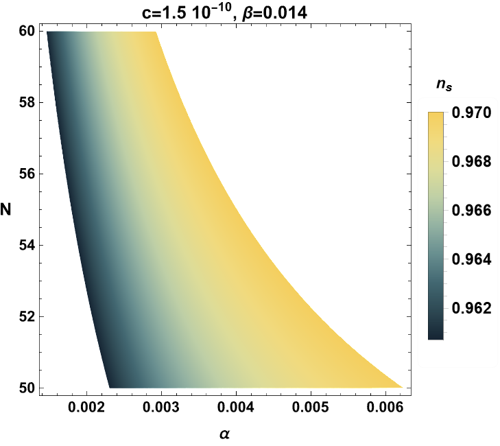
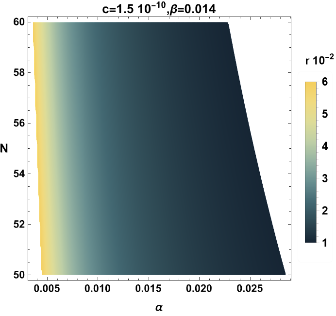
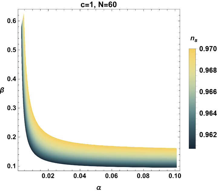
The corresponding value for the scalar spectral index is , and the scalar to tensor ratio is . For generic points of , acceptable values of the scalar index and the scalar to tensor ratio are illustrated in the left and the right of Fig.(1), respectively. In certain regions of the moduli space, the obtained results match
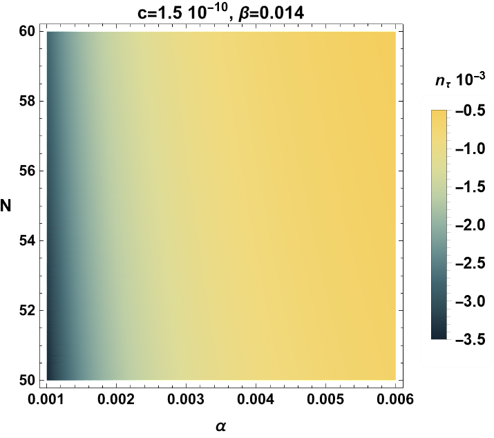
perfectly with the Planck constraints, where the corresponding values are represented by an ivory tan tiled color. For the point , moreover, we find that the value of the tensor index is . The stringy constraint is also verified, where we obtain and . Certain cosmological values corresponding to generic points of the moduli space are represented in Fig.(2). In such a figure, the values of the tensor spectral index are provided by taking the different values of the e-folding number and the scaling parameter .
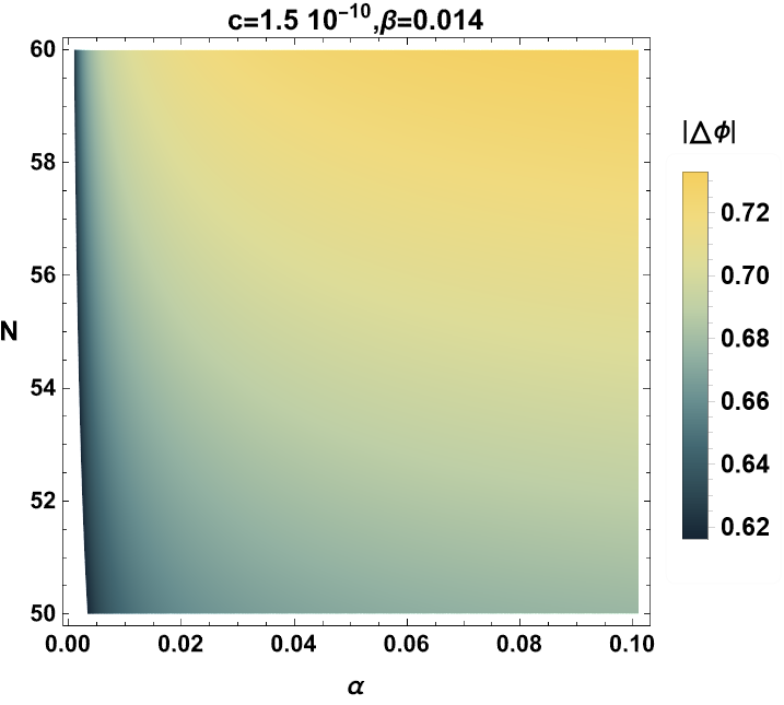
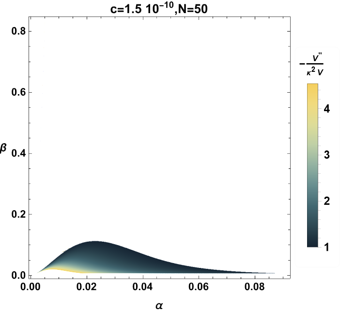
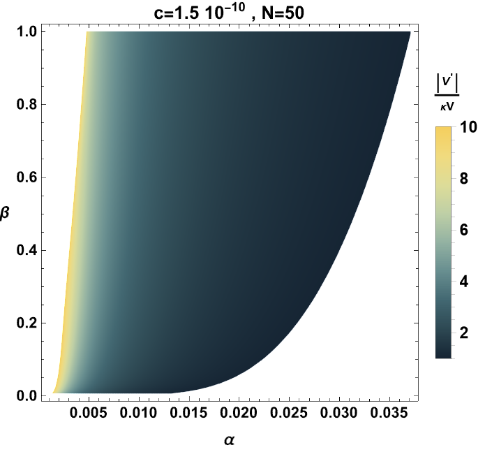
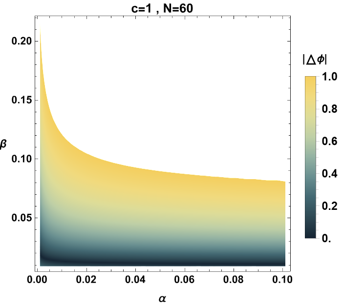
Concerning the swampland criteria, the relevant quantities and are discussed by varying of the free parameter and the rescaling parameter . Indeed, the initial and the final values of the field which are found to be and providing being in accordance with the distance conjecture. This value lays in the dark teal region of Fig.(3). For the de Sitter conjectures, we get values consistent with the swampland criteria. For the runway instability, we obtain , located at the dark teal region illustrated in the right of Fig.(4). The tachyonic instability is found to be , laying at the ivory tan region being represented in the left of Fig.(4). In the present rescaled gravity model, we have obtained values greater than showing that one has acceptable conditions.
The chosen range for the free parameter is motivated by the fact that the rescaling parameter is at most equal to one, according to the previous discussion. Following to a numerical analysis for , we get . To avoid large field values, we consider the following choice . One should note that the main objective is not just to meet observational data, but also to extract the swampland regions in the moduli space. The arbitrary values of such free parameters could produce models which could be checked for consistency with quantum gravity being a basic approach of the present investigation.
 |
 |
We also highlight the numerical values of the inflationary indices, which are as follows , , and . The sound velocity is practically which is consistent with the absence of instability. The scalar potential value for the obtained set of the slow-roll indices is , where the order of the potential seems to be related to the integration constant via the relation .
Via a qualitative analysis, we can observe that the landscape is surrounded by a vast swampland of consistent-looking semi-classical EFTs corresponding to the union of all the moduli space regions verifying the conditions checked above. The presence of such a vast behavior indicates a degree of consistency of the EFTs with quantum gravity.
4.1.2 -model
In this part, we consider the -model. In particular, we use similar computations performed in the previous model. Indeed, the solution of Eq.(4.9), giving positive field values, is
| (4.15) |
For this model, the real solution of Eq.(4.11) is
| (4.16) |
where one has used
| (4.17) |
To get the numerical values of the relevant quantities, one should consider a point in the moduli space with the reduced units. In particular, we take the point of . Indeed, the values for the scalar spectral index and the tensor-to-scalar ratio are and , respectively. This model is incompatible with the Planck data where the maximum value of the scalar spectral index seems to be around the point , as detected in Fig.(5).
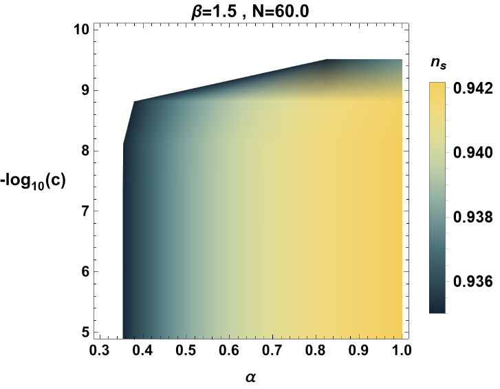
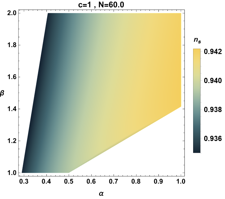 |
In the left panel of Fig.(5), the values of are represented in the colored bar by varying the integration constant and the rescaling parameter . In the right panel of Fig.(5), the values of are represented by varying the free parameter and the rescaling parameter . It follows from this figure that the maximal value of lays in the regions defined by the constraints , and . However, the scalar to the tensor ratio and the tensor spectral index are found to be and , respectively. These two last values match perfectly with the observational data.
The illustrated interval of is constrained by the mentioned conditions on and parameters. The regions that are not shown are not relevant. For , the values of are not even close to acceptable ones. For , moreover, the values of are independent of .
The incompatibility of the scalar spectral index with the observational data allows one to rule out such a model without moving into the swampland criteria analysis.
4.1.3 -model
For this model, we find that the final value of the scalar field is
| (4.18) |
where we have used
| (4.19) |
The real and positive solution of Eq.(4.11) is
| (4.20) |
Now, we consider the point of the moduli space . At such a point, we find that the scalar spectral index is . The scalar to tensor ratio is found to be . For generic points of , the obtained values of the scalar index are illustrated in Fig.(6).
A close examination shows that one has found acceptables values matching perfectly with the Planck constraints, where the values corresponding to are represented by a dark teal color.
After computations, we find that the numerical value of the tensor index is . It has been remarked that the stringy constraint is also satisfied, where we obtain leading to .
Regarding the swampland criteria, we investigate the associated conditions. Indeed, we can first calculate the initial and the final values of the scalar field. They are found to be and , respectively. Such values provide showing an inconsistent behavior with the distance conjecture. The constraints on the scalar index and the distance conjecture are satisfied separately. The values that are bounded by the distance conjecture of are represented in Fig.(7).
In this figure, the obtained values of the relevant quantity are represented in the colored bar by varying the free parameter and the rescaling parameter . The discrepancy between the two conditions is apparent in the two previous figures, where it is clear that the two consistency regions never intersect. For the de Sitter conjectures, we get values consistent with the swampland criteria. For the runway instability, we obtain while the tachyonic instability is found to be . In the present rescaled gravity model, we obtain values greater than revealing that one has acceptable conditions.
4.2 Discussion on the remaining -models
Instead of repeating the above treatment, we prefer to provide the relevant results of the remaining models. We start by noting that the -model should be excluded, due to the absence of the real initial field values. To see that, we consider the solution
| (4.21) |
In this equation, we have used
| (4.22) | |||||
| (4.23) |
where one has . For the solution to be real, one must have . However, it has been shown that this is contradictory since one has the condition . Similar behaviors have been remarked for the -model. In fact, Eq.(4.11) has only two considerable solutions. Explicitly, we have
| (4.24) |
It is worth noting that two other solutions generate negative field values, which are omitted by physical constraints. We see clearly that the equation has the real solution with multiplicity equal to 3. The first solution of Eq.(4.2) gives relatively large field values with the condition . This results in vanishingly small values of the scalar coupling derivative , being omitted due to analytical arguments. For the second solution, we basically get completely inconsistent results with the Planck data. Thus, this model should be ruled out.
Lastly, we consider the -model. It is worth noting that the associated coupling constant is not considered as a free parameter. Using the boundary conditions on the scalar coupling function, we find that meaning that this quantity is not independent of the model free parameters. In fact, it provides a reduced moduli space. In Tab. (1), we collect the obtained numerical values of the dealt with quantities and the swampland criteria.
-model for the point
For the chosen moduli space point, it has been observed for this table that the obtained numerical values are acceptable for phenomenological interest. They could be corroborated by certain observational data.
5 Conclusions and discussions
Inspired by differential equations involving special functions, we have presented an algorithm allowing one to get new hypergeometric type scalar potentials from the stringy correction function , coupled to the Gauss-Bonnet term. In particular, we have constructed and analyzed certain models of phenomenological interest by providing inflationary predictions of the relevant cosmological observables. In particular, we have furnished a family models, refereed to as -models where the couple is constrained from the hypergeometric potential behaviors and certain physical arguments. We have shown that these models provide corroborated findings. Using the falsification scenario, we have confronted the predictions brought by the obtained models with the Planck observational data for such a stringy rescaled gravity. Then, we have approached the corresponding swampland conjectures. Among others, we have found that the swampland criteria are satisfied for small values of the slow-roll parameters.
The present work comes up with some sets of questions. A natural question concerns the implementation of extra stringy corrections including the kinetic Einstein coupling. It is possible that such contributions could be useful to produce consistent models via the swampland program. The second question may concern the naturalness arguments of the proposed physical theories. Such questions could be addressed in future investigations.
Data availability statements: Data sharing is not applicable to this article.
Acknowledgements: Saad Eddine Baddis would like to thank H. Belmahi for comments on an early draft of this work. He thanks the organizers of the String-Math 2024, the Abdus Salam International Centre for Theoretical Physics (ICTP), Trieste, Italy, for hospitality. He would like also to thank C. Vafa for discussions and for certain clarifications at ICTP.
References
- [1] C. Vafa, The String Landscape and the Swampland, arXiv:hep-th/0509212.
- [2] N. B. Agmon, A. Bedroya, M. J. Kang, C. Vafa, Lectures on the string landscape and the Swampland, arXiv:2212.06187[hep-th].
- [3] E. Palti, C. Vafa, Timo Weigand, Supersymmetric Protection and the Swampland, arXiv:2003.10452 [hep-th].
- [4] G. Obied, H. Ooguri, L. Spodyneiko and C. Vafa, De Sitter Space and the Swampland, arXiv:1806.08362[hep-th].
- [5] D. Lust, E. Palti and C. Vafa, AdS and the Swampland, Phys. Lett. B 797, 134867(2019), arXiv: 1906.05225[hep-th].
- [6] H. Ooguri and C. Vafa, On the Geometry of the String Landscape and the Swampland, Nucl. Phys. B 766, 21(2007), hep-th/0605264.
- [7] M. Green, J. Schwarz and E. Witten, Superstring Theory, vol 1 and 2, Combridge University Press, 1987.
- [8] J. Polchinski, String theory, vol 1 and 2, Cambridge University Press, 1999.
- [9] C. Vafa, Lectures on Strings and Dualities, arXiv:hep-th/9702201.
- [10] M. Montero, C. Vafa, I. Valenzuela, The Dark Dimension and the Swampland, J. High Energ. Phys. 02, 22(2023).
- [11] J. A. P. Law-Smith, G. Obied, A. Prabhu, C. Vafa, Astrophysical Constraints on Decaying Dark Gravitons, arXiv:2307.11048[hep-ph].
- [12] L. Anchordoqui, I. Antoniadis, D. Lust, The Dark Dimension, the Swampland, and the Dark Matter Fraction Composed of Primordial Black Holes, Phys. Rev. D, 10651(2022), arXiv:2206.07071[hep-th].
- [13] A. D. Linde, Generation Of Isothermal Density Perturbations In The Inflationary Universe, JETP Lett. 40, 1333 (1984), Pisma Zh. Eksp. Teor. Fiz. 40, 496 (1984).
- [14] A. D. Linde, A new inflationary universe scenario: A possible solution of the horizon, flatness, homogeneity, isotropy and primordial monopole problems, Phys. Lett. B108, 389 (1982).
- [15] A. H. Guth and P.J. Steinhardt, The inflationary universe, Scientific American 250, 129 (1984).
- [16] A. D. Linde, A New Inflationary Universe Scenario: A Possible Solution of the Horizon, Flatness, Homogeneity, Isotropy and Primordial Monopole Problems, Phys. Lett. B 108, 393 (1982).
- [17] A.H. Guth and S.Y. Pi, Fluctuations in the New Inflationary Universe, , Phys. Rev. Lett. 49, 1110 (1982).
- [18] D. Polarski and A.A. Starobinsky, Spectra of perturbations produced by double inflation, with an intermediate matter-dominated stage, Nucl. Phys. B385, 623 (1992).
- [19] A.A. Starobinsky, Robustness of the inflationary perturbation spectrum to trans-Planckian physics, PismaZh.Eksp.Teor.Fiz.73, 415 (2001), JETP. Lett. 73, 371 (2001).
- [20] A. H. Guth, The Inflationary Universe: A Possible Solution to the Horizon and Flatness Problems, Phys. Rev. D 23, 356(1981).
- [21] A. Belhaj, M. Benali, Y. Hassouni, M. Oualaid and M. B. Sedra, On brane cosmological behaviors of Starobinsky inflationary model, Int. J. Mod. Phys. A 37, 2250043(2022).
- [22] A. Belhaj, Y. Hassouni, M. Oualaid and M. B. Sedra, On stringy inflation potentials, Mod. Phys. Lett. A 36, 2150225(2021).
- [23] G. Bao-Min, S. Fu-Wen, K. Yang and Z. Yu-Peng, Primordial black holes from valley, Phys. Rev. D 107, 023519 (2023), arXiv:2207.09968 [astro-ph.CO].
- [24] N. Shiníchi and O. D. Sergei, Dark energy, inflation and dark matter from modified F(R) gravity, TSPU Bulletin N 8,(110) 7(2011), arXiv:0807.0685 [hep-th].
- [25] V. K. Oikonomou, Unifying inflation with early and late dark energy epochs in axion gravity, Phys. Rev. D 103, 044036(2021), arXiv:2012.00586[astro-ph.CO].
- [26] S. Kachru et al. textitde Sitter vacua in string theory, Phys. Rev. D 68, 046005(2003), hep-th/0301240.
- [27] C. Beasley and E. Witten,Topological phase, spin Chern-Simons theory and level rank duality on lens space, JHEP 07, 046(2002), hep-th/0203061.
- [28] B.S. Acharya, F. Denef and R. Valandro, Statistics of M theory Vacua, JHEP 06, 056(2005), hep-th/0502060.
- [29] I. Sawicki and W. Hu, Stability of Cosmological Solution in f(R) Models of Gravity, Phys. Rev. D 75, 127502(2007), arXiv:astro-ph/0702278.
- [30] A.D. Linde, Extended Chaotic Inflation and Spatial Variations of the Gravitational Constant , Phys. Lett. B238, 160 (1990).
- [31] J. García-Bellido, A.D. Linde and D.A. Linde, Fluctuations of the gravitational constant in the inflationary Brans-Dicke cosmology, Phys. Rev. D 50, 730 (1994).
- [32] S. Carloni, Covariant gauge invariant theory of Scalar Perturbations in -gravity: a brief review, Open Astron. J 3, 76(2010), arXiv:1002.3868[gr-qc].
- [33] T. P. Sotiriou, f(R) gravity and scalar-tensor theory, Class. Quant. Grav. 23, 5117(2006), arXiv:gr-qc/0604028[gr-qc].
- [34] S. D. Odintsov and V. K. Oikonomou,Unification of Inflation with Dark Energy in Gravity and Axion Dark Matter, Phys. Rev. D 99, 104070(2019), arXiv:1905.03496[gr-qc].
- [35] A. Belhaj, S.E. Ennadifi, M. Lamaaoune, On inflation and axionic dark matter in a scaled gravity, Eur. Phys. J.Plus 139 2, 147(2024), arXiv:2402.01301.
- [36] A. Belhaj, M. Benali, S.E. Ennadifi, M. Lamaaoune, On inflation scenarios and dark energy in a scaled gravity, Int. J. Geom. Meth. Mod. Phys. 20, 2350167(2023).
- [37] A. Belhaj, M. Benali, M. Lamaaoune, On inflation potentials in kinetic coupling scenarios, Mod. Phys. Lett.A 38, 2350008(2023).
- [38] A. Belhaj, M. Benali, Y. Hassouni, M. Lamaaoune, On inflationary models in f(R,T) gravity with a kinetic coupling term, Int.J. Mod. Phys. A 38, 2350043(2023).
- [39] Y. Akrami et al. Planck 2018 results. X. Constraints on inflation, Astron. Astrophys. 641, 10(2020), arXiv:1807.06211.
- [40] N. Aghanim et al., Planck 2018 results. VI. Cosmological parameters, Astron. Astrophys. 641, 6(2020), arXiv:1807.06209[astro-ph.CO].
- [41] P. A. R. Ade et al., Improved Constraints on Primordial Gravitational Waves using Planck, WMAP, and BICEP/Keck Observations through the 2018 Observing Season, Phys. Rev. Lett. 127, 151301(2021), arXiv:2110.00483[astro-ph.CO].
- [42] A. Albrecht and P. J. Steinhardt,title, Phys. Rev. Lett. 48, 1220(1982).
- [43] P. Candelas, G. Horowitz, A. Strominger, E. Witten, Vacuum configurations for super- strings, Nucl. Phys. B 258, 46(1985).
- [44] B.R. Greene, String Theory on Calabi Yau Manifolds, arXiv:hep-th/9702155.
- [45] S. Nojiri, S. D. Odintsov and V. K. Oikonomou, Modified Gravity Theories on a Nutshell: Inflation, Bounce and Late-time Evolution, Phys. Rept. 692, 104(2017), arXiv:1705.11098 [gr-qc].
- [46] S. D. Odintsov, D. Sáez-Chillón Gómez and G. S. Sharov, Exponential F(R) gravity with axion dark matter, Phys. Dark Univ. 42 , 101369(2023), arXiv:2310.20302 [gr-qc].
- [47] S. D. Odintsov and V. K. Oikonomou, Aspects of Axion Gravity, EPL 129, no.4, 40001(2020), arXiv:2003.06671 [gr-qc].
- [48] I.D. Gialamas, A. Karam, A. Lykkas and T.D. Pappas, Palatini-Higgs inflation with non-minimal derivative coupling, Phys. Rev. D 102, no.6, 063522(2020), arXiv:2008.06371[gr-qc].
- [49] S. D. Odintsov and V. K. Oikonomou, Gravity Inflation with String-Corrected Axion Dark Matter, Phys. Rev. D 99, 064049(2019), arXiv:1901.05363 [gr-qc].
- [50] S. D. Odintsov, V. K. Oikonomou, I. Giannakoudi, F. P. Fronimos and E. C. Lymperiadou, Recent Advances in Inflation, Symmetry 15, 1701(2023), arXiv:2307.16308 [gr-qc].
- [51] V. K. Oikonomou, Konstantinos-Rafail Revis, Ilias C. Papadimitriou, Maria-Myrto Pegioudi, Swampland Criteria and Constraints on Inflation in a f(R,T) Gravity Theory, Int. J. Mod. Phys. D32, 2350034(2023).
- [52] V. K. Oikonomou, I. Giannakoudi, A. Gitsis, K-R Revis, Rescaled Einstein-Hilbert Gravity: Inflation and the Swampland Criteria, Int.J.Mod.Phys.D 31, 02, 2250001(2022), arXiv:2105.11935.
- [53] V. K. Oikonomou, Rescaled Einstein-Hilbert Gravity from f(R) Gravity: Inflation, Dark Energy and the Swampland Criteria, Phys. Rev. D 103, 124028(2021), arXiv:2012.01312.
- [54] P. Chaturvedi, U. Kumar, U. Thattarampilly, V. Kakkat, Exact rotating black hole solutions for f(R) gravity by modified Newman Janis algorithm, Eur.Phys.J.C 83 1124(2023), arXiv:2309.17044 [gr-qc].
- [55] O. Lacombe, S. Mukohyama, J. Seitz, Are f(R,Matter)f(R,Matter) theories really relevant to cosmology?, JCAP 05, 064 (2024), arXiv:2311.12925 [gr-qc].
- [56] A. Gitsis, K. R. Revis, S.A. Venikoudis, F.P. Fronimo, Swampland criteria for rescaled Einstein- Hilbert gravity with string corrections, arXiv:2301.08126 [gr-qc].
- [57] J. C. Hwang and H. Noh, Classical evolution and quantum generation in generalized gravity theories including string corrections and tachyon: Unified analyses, Phys. Rev. D 71, 063536(2005), arXiv:gr-qc/0412126 [gr-qc].
- [58] D. J. Gogoi, U. D. Goswami, Gravitational Waves in f(R) Gravity Power Law Model, Indian Journal of Physics 96, 637 (2022), arXiv:1901.11277 [gr-qc].
- [59] D. J. Gogoi, U. D. Goswami, A new f(R) Gravity Model and properties of Gravitational Waves in it, Eur. Phys. J. C 80, 1101 (2020), arXiv:2006.04011 [gr-qc].
- [60] L. G. Jaime, L. Patiño, M. Salgado, About matter and dark-energy domination eras in gravity or lack thereof, Phys. Rev. D 87, 024029(2013), arXiv:1212.2604 [gr-qc].
- [61] B. P. Abbott et al. GW170817: Observation of Gravitational Waves from a Binary Neutron Star Inspiral [LIGO Scientific and Virgo], Phys. Rev. Lett. 119, 16110 (2017), arXiv:1710.05832 [gr-qc].
- [62] B. P. Abbott et al. Multi-messenger Observations of a Binary Neutron Star Merger, Astrophys. J. Lett. 848, no.2, L12 (2017), arXiv:1710.05833 [astro-ph.HE].
- [63] B. P. Abbott et al. Gravitational Waves and Gamma-rays from a Binary Neutron Star Merger: GW170817 and GRB 170817A, [LIGO Scientific, Virgo, Fermi-GBM and INTEGRAL], Astrophys. J. Lett. no.2, L13, 848 (2017), arXiv:1710.05834 [astro-ph.HE].
- [64] B. P. Abbott et al. GW170817: Measurements of Neutron Star Radii and Equation of State, [LIGO Scientific and Virgo], Phys. Rev. Lett. 121, 161101 (2018), arXiv:1805.11581 [gr-qc].
- [65] B. P. Abbott et al. Properties of the binary neutron star merger GW170817, [LIGO Scientific and Virgo], Phys. Rev. X 9, 011001 (2019), arXiv:1805.11579 [gr-qc].
- [66] J. M. Ezquiaga and M. Zumalacarregui, Dark Energy after GW170817: dead ends and the road ahead, Phys. Rev. Lett. 119, 251304 (2017), arXiv:1710.05901 [astro-ph.CO].
- [67] J. Sakstein and B. Jain, Implications of the Neutron Star Merger GW170817 for Cosmological Scalar-Tensor Theories, Phys. Rev. Lett. 119, 251303 (2017), arXiv:1710.05893 [astro-ph.CO].
- [68] B. P. Abbott et al. Tests of General Relativity with GW170817, [LIGO Scientific and Virgo], Phys. Rev. Lett. 123, 011102( 2019), arXiv:1811.00364 [gr-qc].
- [69] H. Chun Sun, Y. Zhu H. Xu, et al, Searching for the nano-Hertz stochastic gravitational wave background with the Chinese Pulsar Timing Array Data Release I, Res.Astron.Astrophys. 23, 075024 (2023), arXiv:2306.16216 [astro-ph.HE].
- [70] G. Agazie, et al, The NANOGrav 15-year Data Set: Evidence for a Gravitational-Wave Background, Astrophys.J.Lett. L8, 951 (2023), arXiv:2306.16213 [astro-ph.HE].
- [71] Daniel J. Reardon, et al, Search for an isotropic gravitational-wave background with the Parkes Pulsar Timing Array, Astrophys.J.Lett. L6, 951(2023), arXiv:2306.16215 [astro-ph.HE].
- [72] J. Antoniadis, at al, The second data release from the European Pulsar Timing Array III. Search for gravitational wave signals, Astron. Astrophys. A94, 685 (2024), arXiv:2306.16214 [astro-ph.HE].
- [73] N. Aghanim et al. [Planck],Planck 2018 results. VI. Cosmological parameters, Astron. Astrophys. 641 (2020), A6 [erratum: Astron. Astrophys.] C4 652 (2021), arXiv:1807.06209 [astro-ph.CO].
- [74] S. A. Venikoudis and F. P. Fronimos, Inflation with Gauss-Bonnet and Chern-Simons higher-curvature-corrections in the view of GW170817, Gen. Rel. Grav. 53, 75 (2021), arXiv:2107.09457 [gr-qc].
- [75] S.D. Odintsov, V.K. Oikonomou, F.P. Fronimos, K.V. Fasoulakos, Unification of a Bounce with a Viable Dark Energy Era in Gauss-Bonnet Gravity, Phys. Rev. D102, 104042 (2020), arXiv:2010.13580 [gr-qc].
- [76] S. D. Odintsov, V. K. Oikonomou and F. P. Fronimos, Rectifying Einstein-Gauss-Bonnet Inflation in View of GW17081, Nucl. Phys. B958, 115135 (2020), arXiv:2003.13724 [gr-qc].