Over-rotation coherent error in quantum gates subjected to pseudo twirling
Abstract
Quantum error mitigation schemes (QEM) have greatly enhanced the efficiency of quantum computers, specifically focusing on reducing errors caused by interactions with the environment. Nevertheless, the presence of coherence errors, typically arising from miscalibration and inter-qubit crosstalk, is a significant challenge to the scalability of quantum computing. Such errors are often addressed using a refined Pauli twirling scheme called Randomized Compiling (RC) that converts the coherent errors into incoherent errors that can then be mitigated by conventional QEM. Unfortunately for multi-qubit gates, RC is restricted to Clifford gates such as CNOT and CPHASE. However, it has been demonstrated experimentally that a direct implementation of multi-qubit non-Clifford gates, i.e. without using multi-qubit Clifford gates, has reduced the depth of the circuit by a factor of four and more. Recently, a framework called pseudo-twirling (PST) for treating coherent error in multi-qubit non-Clifford gates has been introduced and experimentally demonstrated. We show analytically that a higher order correction to the existing PST theory yields an over-rotation coherent error generated by the PST protocol itself. This PST effect has no analogue in RC. Although the small induced over-rotation can amount to a significant coherent error in deep circuits, we explain why it does not degrade the performance of the gate.
I Introduction
Two types of errors impede the performance of quantum computers: 1) incoherent errors (“noise”) that arise due to the interaction of the qubits with the environment, and 2) coherent errors that typically occur due to miscalibration or crosstalk interaction between the qubits. While incoherent errors can be addressed by a plethora of quantum error mitigation (QEM) techniques [1, 2, 3, 4, 5, 6, 7, 8, 9, 10], until recently, the only proven tools for addressing coherent errors was Pauli twirling (PT), and its extended version known as ’randomized compiling’ (RC) [11, 12, 13, 14]. Unlike PT, under some restrictions RC can also handle single-qubit non-Clifford gates. In PT/RC, an ensemble of random circuits is created by padding the multi-qubit Clifford gate by Pauli gates, which, in the absence of coherent error, do not alter the functionality of the Clifford gate. The ensemble average cancels the odd orders of the coherent error, and the remaining even orders manifest as incoherent error that can be addressed by QEM. This effect is expected since the ensemble average is a mixture of unitaries (if there are no incoherent errors), thereby reducing the purity of the final state.
Non-Clifford gates are crucial for achieving quantum advantage because without them circuits can be efficiently simulated on a classical computer. In the standard CNOT (or CPhase) paradigm, all non-Clifford gates are low-noise single-qubit gates. While this choice is sensible, it has the drawback that any departure from a two-qubit Clifford gate requires at least two CNOT operations, which substantially increase the runtime and the exposure to incoherent error mechanisms. Non-Clifford two-qubit gates naturally arise in lattice simulations (e.g., transverse Ising model), quantum Fourier transform, QAOA circuits, and more. In a previous studies, it was experimentally demonstrated that using multi-qubit non-Clifford (MQNC) gates reduced circuit depth by a factor of four [15] and six [16], leading to a significant decrease in overall noise levels within the circuit. Unfortunately, since PT and RC cannot be applied to these gates, they are susceptible to calibration and crosstalk errors. A formalism called pseudo twirling (PST) for addressing coherent errors in MQNC gates was recently introduced [17]. Earlier descriptions of the PST protocol, lacking supporting theory (see the discussion that will appear in v3 of [17]), are found in [18, 19].
Another method for addressing coherent and incoherent errors in non-Clifford gates has been introduced in [20]. Unfortunately, the sampling overhead of this method is highly non-scalable. Furthermore, since it is based on noise learning, it is inherently sensitive to time variations in the noise profile. While PT and PST require the implementation of many circuits, they do not involve a sampling overhead. The total number of shots needed to achieve the target accuracy without twirling is evenly distributed among the different twirling circuits.
The key differences between PST and PT are: the specific types of coherent errors addressed, the nature of the resulting noise channel, and the level of control necessary to execute these protocols. Due to these distinctions, one method cannot be considered as a special case of the other. Beginning with the first difference, PT treats all types of coherent errors by converting them into noise, whereas PST excludes a particular type of coherent error: controlled mis-rotations. This difference has an important operational implication. Unlike PT, PST can be applied during the gate calibration stage. The advantage of employing PST in high-accuracy calibration protocols was experimentally demonstrated in [17]. Secondly, PT transforms coherent errors into Pauli errors, i.e. the noise has a diagonal form in the Pauli basis, whereas PST, in the first order, renders the error channel Hermitian with off-diagonal elements in the Pauli basis. Finally, PT only requires the ability to implement single-qubit Pauli gates, whereas PST also requires altering the sign of the driving amplitude. Yet this operational advantage of PT is irrelevant when it comes to multi-qubit non-Clifford gates where PT is not applicable.
Our work highlights an intriguing aspect that further distinguishes PST from PT: the contribution of a second-order Magnus term introduces a small coherent error by causing a slight over-rotation in the driving field. While this might initially appear problematic, given that the primary aim of PST is to eliminate coherent errors, we explain why this specific type of coherent error can generally be disregarded in most scenarios. The analysis presented in [17] is grounded in the first-order Magnus expansion. This approximation proves effective even in situations where errors are significant [21]. However, it is possible that for certain purposes, such as high-accuracy calibration, the influence of the second order term cannot be overlooked. The objective of this paper is to explicitly determine the impact of the next order. In doing so, we also establish a clear operational regime for the first-order approximation.
The paper starts in Sec. II with some preliminaries and a short review of the PST formalism. In Sec. III we evaluate the term for arbitrary coherent error. Section IV studies the impact of incoherent noise and higher order correction using parity arguments. Finally, in Section V we conclude and discuss the implications of the term for practical applications.
II Preliminaries
II.1 Introduction To Liouville space
The evolution of an isolate quantum system is described by the Liouville von Neumann equation
| (1) |
where , the density matrix that describes the quantum state, is a matrix and is the Hilbert space dimension of the system. Liouville space is an alternative formulation where the density matrix is flattened into a density vector of dimension [22]. In Liouville space, the quantum dynamics (1) translates into a Schrödinger-like equation
| (2) |
where the Liouville Hamiltonian is related to the Hilbert space Hamiltonian through , where stands for transposition. The evolution operator that propagates the quantum state in Liouville space can be expressed as
| (3) |
where, is the evolution operator in Hilbert space . Pauli matrices in Liouville space can either appear as Hamiltonians or as unitaries, but unlike in Hilbert space, these two forms differ. Let us denote by the tensor product of single-qubit Pauli matrices such that . A Pauli Hamiltonian in Liouville space is given by , while according to Eq. (3), a Pauli evolution operator has the form in Liouville space. These two Pauli forms are related via . In particular, we shall use the fact that Pauli unitaries always commute in Liouville space while two Pauli Hamiltonians in Liouville commute (anti commute) if their corresponding Paulis in Hilbert space commute (anti commute). The same holds the commutation relation between Pauli unitaries and Pauli Hamiltonians . Finally, while is equal to the identity operator is not equal to the identity.
II.2 Overview of the PST formalism
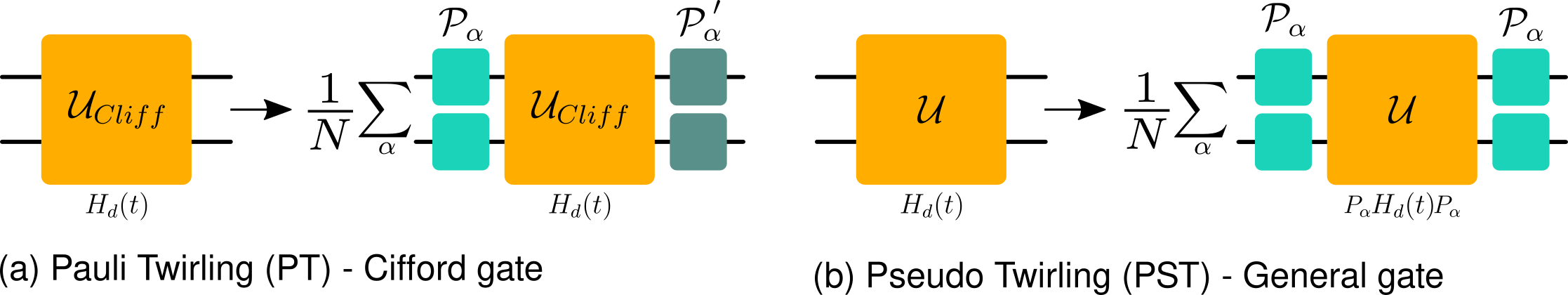
To illustrate the pseudo-twirling protocol studied in [17], we begin with a straightforward example. Consider the following non-Clifford two-qubit gate where and . In analogy to PT, our goal is to create an operation that retains the functionality of the ideal gate. When twirling using , we find that because commutes with . In contrast, anti-commutes with , resulting in . The PST protocol leverages the fact that if Pauli operators anti-commute with the Hamiltonian that generates (or equivalently in Liouville space), the desired transformation can be achieved by reversing the angle, i.e., changing the sign of the driving fields. The difference between Pauli twirling and pseudo twirling is shown in Fig. 1.
In a broader context, when the driving Hamiltonian is composed of multiple Pauli terms, the evolution operator becomes . The Pseudo Twirling (PST) protocol can be mathematically expressed as
| (4) |
where equals if and commute or anti-commute, respectively. Note that in the definition of , Pauli matrices in Hilbert space are used. Mathematically, expression (4) is straightforward in the absence of coherent error. Operationally, at the beginning of the protocol, the appropriate is applied. Next, a modified unitary function is executed by changing the sign of specific control signals. Finally, another is applied at the end of the gate. Importantly, the Hamiltonian of the modified unitary retains the same terms as the original Hamiltonian, with only the signs of some terms changed. Thus, under the assumption that the signs of the driving Hamiltonian terms are controllable, the PST implementation is no more challenging than implementing the original unitary.
PST has two distinctive features compared to randomized compiling. Firstly, it is applicable to non-Clifford gates. Secondly, there is one specific coherent error it cannot average out: a controlled mis-rotation. This latter feature is actually useful for calibration purposes (see [17]).
II.3 PST Theory from Magnus Expansion
In this work we consider a Hamiltonians of the form
| (5) |
where is the drive Hamiltonian that in the absences of coherent error generates the desired unitary . represents the coherent errors we wish to mitigate. Using the Magnus expansion [23] in the interaction picture, one can write the evolution operator at time as
| (6) |
where is the duration of the driving pulse, ,
| (7) | ||||
| (8) |
and is the coherent error in the interaction picture. Since is proportional to and when the coherent error in each gate is small, in previous analysis of the PST protocol all term but the first Magnus terms were neglected. In general, the higher order Magnus terms are difficult to calculate and have a small impact when . However here we show that the second order Magnus term leads to a surprisingly simple result which is the focus of the present paper.
By Taylor expansion of the Magnus term or directly from the Dyson series, one gets that a expansion of order of reads
| (9) |
The application of pseudo twirling leads to following evolution operator [17].
| (10) |
where
| (11) |
and
| (12) |
In [17] it was shown that PST averages to zero the term, and the averaging of over leads to Lindblad dissipation terms that represent the noise associated with PST, i.e. the conversion of coherent error into incoherent errors. Next, we turn to our attention to the averaging of .
III The PST induced over-rotation
Using , we get
| (13) |
However, since as shown in the Appendix of [17], the last term is equal to zero and we finally obtain
| (14) |
where
| (15) |
That is, since the cross terms vanish, it is possible to consider the contribution of each separately and add them with weights. However, if a certain coherent error element commutes with the driving Pauli , it holds that and therefore . Thus, these elements can be omitted from the summation and we have
| (16) |
where is the set of that anti-commutes with . To simplify the integrand in (15) we start with the dressed Hamiltonian expression
| (17) |
Using and (since ) we get the relation
| (18) |
and consequently
| (19) |
Using this result in the integrand of Eq. (15) leads to
| (20) |
For the first term we obtain
| (21) |
and a similar expression holds for the second term. Consequently we get
| (22) |
Finally, after the double integration, and using we obtain our main result
| (23) |
and therefore the effective drive Hamiltonian is
| (24) |
Since for any , the term can be considered as an amplitude amplification factor, or alternatively, as a relative over-rotation. At first, it may seem quite striking that after PST, all the various coherent errors manifest simply as modification of the coefficient in front of the driving Hamiltonian. However, we argue that this must be the case. Had a different term survived after PST we could have applied PST again to eliminate it. Note that even if the survived term had the same sign dependence as that of the drive, PST would still eliminated it (see Sec. III.A in [17]). However, PST of a PST is just a regular PST. This leads to the conclusion that when it comes to residual coherent errors only mis-rotation of the drive is possible. Although we do not study it here, we expect the same logic to be valid for and higher orders in the Magnus expansion.
To verify our theoretical result, Eq. (24), we consider a non-Clifford ZX gate with uncontrolled coherent errors, i.e. independent of the driving . The Hamiltonian
| (25) |
is propagated for a duration . The resulting evolution operator is
| (26) |
Next, we calculate the weight of different terms in the Hamiltonian (effective Hamiltonian) before (after) performing PST. We choose the coherent error in such a way that three components (XX, ZZ, and YX) anti-commute with the original Hamiltonian and one term (YY) commutes with the driving Hamiltonian. Table 1 validates the theoretical prediction Eq. (24) of the PST induced over-rotation. The simulation parameters are , , , and .
| XX | YY | ZZ | YX | ZX (numerics) | ZX PST (theoretical) | |
| No PST | 0.2 | 0.6 | 0.2 | 0.4 | 1 | - |
| PST | 0 | 0 | 0 | 0 | 1.0207 | 1.019 |
IV Parity and higher orders
In this section, we employ a parity argument in order to study third order effects without explicit calculations. In the original frame, i.e. before the transition to the interaction frame, the PST evolution operator is
| (27) |
Next, we consider the case where there exist a Pauly matrix that anti-commutes with . As a result . For any element in the set we choose another element defined as . Thus, if we carry out the sum over in pair of and we get that each pair form an even function of :
| (28) |
Thus, has the form of an even function in : . Consequently, all odd order term in in the Taylor expansion must be zero. In particular the third order in has to be zero.
Importantly, this symmetry can be broken by the present of noise:
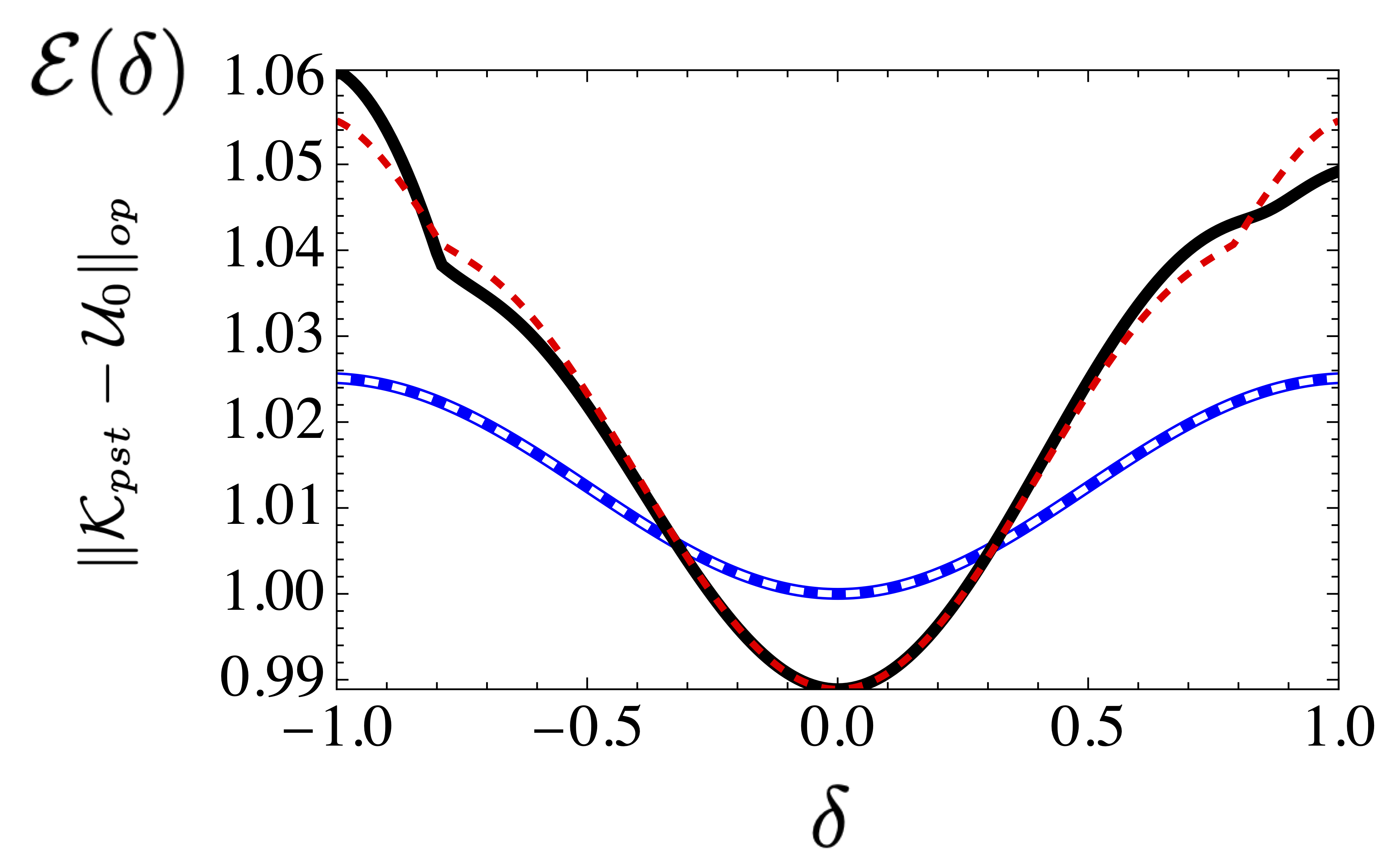
Since in general , the even parity no longer holds. Interestingly, in the important case of Pauli noise , and therefore the symmetry still holds, leading to . In Fig. 2 we plot the error of the PST channel with respect to the ideal channel. We used the same as in Table 1 but with added coefficient that enables control over the amplitude of and the sign of the coherent error. The blue line shows that for a Pauli Z noise (decoherence), is indistinguishable from the symmetrized dashed line . When the noise is an amplitude damping channel (black line), the symmetry of is broken and . However, the difference is small. To observe this difference we use which corresponds to an extreme decay. We also used for making the effect more visible.
V Discussion and operational implications
In practice, when calibrating a gate to generate a rotation of , the drive amplitude (which is proportional to ) is scanned until the monitored expectation value matches its ideal values. In the absence of errors, the scan yields the value . However, in the presence of coherent errors, the scan will lead to a value of that satisfies . We emphasize that the calibration process will determine the correct value of without knowing the values of . As a result, the final accuracy of the gates is not degraded by pseudo-twirling over-rotation effect studied here. The pseudo-twirling over-rotation makes the calibration curve slightly non-linear with respect to the drive amplitude. Consequently, it is not possible to use linearity to automatically calibrate the gate to a different value of . For instance, to achieve half the rotation, one cannot simply set .
In this work, we studied a pseudo-twirling induced coherent error effect (nonlinear over-rotation) arising from the second-order Magnus expansion. It was explained why this term can be safely ignored in most cases. Nevertheless, our findings substantiate the validity and understanding of the pseudo-twirling framework. In particular, by evaluating the second order Magnus term we learn on the validity regime of the previous first order Magnus expansion analysis. Finally, we point out that, in principle, it is possible to measure the non-linearity of the actual rotation with respect to the drive amplitude and deduce the magnitude of the non-commuting coherent errors without carrying out time-consuming process tomography.
VI ACKNOWLEDGMENTS
Raam Uzdin is grateful for support from the Israel Science Foundation (Grant No. 2556/20). The support of the Israel Innovation Authority is greatly appreciated.
References
- [1] Zhenyu Cai, Ryan Babbush, Simon C. Benjamin, Suguru Endo, William J. Huggins, Ying Li, Jarrod R. McClean, and Thomas E. O’Brien. Quantum error mitigation. Rev. Mod. Phys., 95:045005, Dec 2023.
- [2] Suguru Endo, Simon C Benjamin, and Ying Li. Practical quantum error mitigation for near-future applications. Physical Review X, 8(3):031027, 2018.
- [3] Yasunari Suzuki, Suguru Endo, Keisuke Fujii, and Yuuki Tokunaga. Quantum error mitigation as a universal error reduction technique: Applications from the nisq to the fault-tolerant quantum computing eras. PRX Quantum, 3(1):010345, 2022.
- [4] Kristan Temme, Sergey Bravyi, and Jay M Gambetta. Error mitigation for short-depth quantum circuits. Physical review letters, 119(18):180509, 2017.
- [5] William J Huggins, Sam McArdle, Thomas E O’Brien, Joonho Lee, Nicholas C Rubin, Sergio Boixo, K Birgitta Whaley, Ryan Babbush, and Jarrod R McClean. Virtual distillation for quantum error mitigation. Physical Review X, 11(4):041036, 2021.
- [6] Balint Koczor. Exponential error suppression for near-term quantum devices. Physical Review X, 11(3):031057, 2021.
- [7] Andre He, Benjamin Nachman, Wibe A. de Jong, and Christian W. Bauer. Zero-noise extrapolation for quantum-gate error mitigation with identity insertions. Phys. Rev. A, 102:012426, Jul 2020.
- [8] Armands Strikis, Dayue Qin, Yanzhu Chen, Simon C Benjamin, and Ying Li. Learning-based quantum error mitigation. PRX Quantum, 2(4):040330, 2021.
- [9] Ying Li and Simon C Benjamin. Efficient variational quantum simulator incorporating active error minimization. Physical Review X, 7(2):021050, 2017.
- [10] Sergei Filippov, Matea Leahy, Matteo AC Rossi, and Guillermo García-Pérez. Scalable tensor-network error mitigation for near-term quantum computing. arXiv preprint arXiv:2307.11740, 2023.
- [11] Joel J Wallman and Joseph Emerson. Noise tailoring for scalable quantum computation via randomized compiling. Physical Review A, 94(5):052325, 2016.
- [12] Akel Hashim, Ravi K. Naik, Alexis Morvan, Jean-Loup Ville, Bradley Mitchell, John Mark Kreikebaum, Marc Davis, Ethan Smith, Costin Iancu, Kevin P. O’Brien, Ian Hincks, Joel J. Wallman, Joseph Emerson, and Irfan Siddiqi. Randomized compiling for scalable quantum computing on a noisy superconducting quantum processor. Phys. Rev. X, 11:041039, Nov 2021.
- [13] Noah Goss, Samuele Ferracin, Akel Hashim, Arnaud Carignan-Dugas, John Mark Kreikebaum, Ravi K Naik, David I Santiago, and Irfan Siddiqi. Extending the computational reach of a superconducting qutrit processor. arXiv preprint arXiv:2305.16507, 2023.
- [14] Zhenyu Cai and Simon C Benjamin. Constructing smaller pauli twirling sets for arbitrary error channels. Scientific reports, 9(1):11281, 2019.
- [15] Youngseok Kim, Christopher J Wood, Theodore J Yoder, Seth T Merkel, Jay M Gambetta, Kristan Temme, and Abhinav Kandala. Scalable error mitigation for noisy quantum circuits produces competitive expectation values. Nature Physics, pages 1–8, 2023.
- [16] John PT Stenger, Nicholas T Bronn, Daniel J Egger, and David Pekker. Simulating the dynamics of braiding of majorana zero modes using an ibm quantum computer. Physical Review Research, 3(3):033171, 2021.
- [17] Jader P Santos, Ben Bar, and Raam Uzdin. Pseudo twirling mitigation of coherent errors in non-clifford gates. arXiv e-prints, pages arXiv–2401, 2024.
- [18] David Layden, Guglielmo Mazzola, Ryan V Mishmash, Mario Motta, Pawel Wocjan, Jin-Sung Kim, and Sarah Sheldon. Quantum-enhanced markov chain monte carlo. Nature, 619(7969):282–287, 2023.
- [19] I-Chi Chen, Benjamin Burdick, Yongxin Yao, Peter P Orth, and Thomas Iadecola. Error-mitigated simulation of quantum many-body scars on quantum computers with pulse-level control. Physical Review Research, 4(4):043027, 2022.
- [20] David Layden, Bradley Mitchell, and Karthik Siva. Theory of quantum error mitigation for non-clifford gates. arXiv preprint arXiv:2403.18793, 2024.
- [21] Ivan Henao, Jader P. Santos, and Raam Uzdin. Adaptive quantum error mitigation using pulse-based inverse evolutions. npj Quantum Information, 9(1):120, 2023.
- [22] Jerryman A Gyamfi. Fundamentals of quantum mechanics in liouville space. European Journal of Physics, 41(6):063002, 2020.
- [23] Sergio Blanes, Fernando Casas, Jose-Angel Oteo, and Jose Ros. The magnus expansion and some of its applications. Physics reports, 470(5-6):151–238, 2009.