Comparing Causal Inference Methods for Point Exposures with Missing Confounders: A Simulation Study

Abstract

[Abstract]Causal inference methods based on electronic health record (EHR) databases must simultaneously handle confounding and missing data. Vast scholarship exists aimed at addressing these two issues separately, but surprisingly few papers attempt to address them simultaneously. In practice, when faced with simultaneous missing data and confounding, analysts may proceed by first imputing missing data and subsequently using outcome regression or inverse-probability weighting (IPW) to address confounding. However, little is known about the theoretical performance of such ad hoc methods. In a recent paper Levis et al.¹ outline a robust framework for tackling these problems together under certain identifying conditions, and introduce a pair of estimators for the average treatment effect (ATE), one of which is non-parametric efficient. In this work we present a series of simulations, motivated by a published EHR based study² of the long-term effects of bariatric surgery on weight outcomes, to investigate these new estimators and compare them to existing ad hoc methods. While the latter perform well in certain scenarios, no single estimator is uniformly best. As such, the work of Levis et al. may serve as a reasonable default for causal inference when handling confounding and missing data together.

, ,and (2024), A simulation study to compare causal inference methods for point exposures with missing confounders, Statistics in Medicine.

1 Introduction

Electronic health record (EHR) databases contain observational data on large populations collected from patient interactions with a healthcare system over a potentially long time period. Given the sheer quantity of information captured, EHR databases are increasingly seen as a useful data source for research across a variety of clinical and public health settings ^{3, 4, 5}. While randomized control trials (RCT) are often considered the gold standard, they may be infeasible to conduct in certain scenarios due to financial cost associated with running the trial, ethical considerations of randomizing subjects to a potentially harmful or inferior treatment, and/or other logistical concerns. Similar financial constraints and external factors may also make it infeasible to conduct prospective observational studies. In such scenarios when RCTs or prospective observational studies may not be possible, EHR data may allow for headway to be made towards studying the research questions of interest.

Despite their upsides, EHR are not without their own unique challenges that threaten the validity of any statistical analyses conducted using such data. Unlike data in a clinical trial, data in an EHR system are not collected with a given research purpose in mind, but rather are collected to record clinical activity and assist with patient billing. In particular, treatments which patients may receive are not randomly assigned, allowing for the presence of confounding bias⁶. Similarly, information researchers would like to know about a patient may not be recorded at particular visits, or at all, meaning missing data is a fundamental challenge with which researchers must contend⁷.

While both confounding and missing data have their own extensive literatures, few methods have been developed aiming to address both issues simultaneously within a formal framework, with notable exceptions including the recent work of Levis and colleagues¹, and several works preceding it^{8, 9, 10, 11, 12, 13, 14}. In this work, we consider the setting where interest lies in estimating the causal average treatment effect (ATE) of some point exposure on a given outcome in an observational EHR-based study where some of the confounders are missing for a subset of patients.

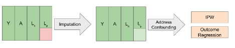
Figure 1: Example analysis pipeline that decomposes the challenges of missing data and confounding as separate tasks. In this example, the analyst first applies imputation to address missing data and then applies their preferred method to deal with confounding.

In practice, when faced with this setting, analysts are likely to employ some ad hoc combination of well known techniques for dealing with missing data and confounding separately, as outlined in Figure 1. For example, one might first use (multiple) imputation to deal with missing data and then feed the resulting imputed dataset(s) into a regression-based analysis to handle confounding. In certain cases such ad hoc approaches may be perfectly reasonable and yield valid results, while in other cases such approaches will not yield valid results.

Levis et al. outlined a formal framework for estimating the causal average treatment effect from cohort studies when confounders satisfy a version of the missing at random (MAR) assumption, and proposed a pair of new estimators for this setting, one of which is an efficient and robust influence function-based estimator that serves as a theoretical benchmark against which such ad hoc methods may be assessed. However no attempt was made to compare the performance of these new estimators to a number of reasonable strategies analysts might attempt in this setting.

In this paper, we seek to use simulations to compare the performance of a number of reasonable approaches one may take when faced with partially missing confounders to the benchmarks outlined in Levis et al.¹, so as to better understand under which scenarios such approaches may be valid and under which scenarios they may be invalid. The simulation settings considered in this work are motivated by the study of long-term outcomes following bariatric surgery. Despite the fact that several clinical trials and observational studies present evidence to suggest that bariatric surgery is the most effective weight-loss treatment for patients with extreme obesity^{15, 16, 17, 18, 19}, the number of patients undergoing bariatric surgery each year is low²⁰. Perhaps that relatively few patients are recommended to undergo bariatric surgery is due to the lack of evidence regarding long-term adverse events, durability of weight loss, and glycemic benefits, especially in comparison to patients who similarly suffer from severe obesity but do not undergo surgery¹⁵. In an ideal world, large scale randomized trials would be conducted to compare long-term outcomes between patients undergoing bariatric surgery to those not undergoing bariatric surgery. Such long-term studies, however, are currently unrealistic and would be slow to generate useful results. Therefore, rigorous and valid EHR-based studies may be the only feasible approach to generate evidence that can inform decisions regarding the long-term effects of bariatric surgery. As such, for these applications and beyond, it will be important to ascertain the operating characteristic of various methods intended to simultaneously handle missing data and confounding bias in these contexts.

2 Background

2.1 Setting and Notation

The problem considered in this paper lies in using data from EHR databases to compare the effectiveness of a finite set of treatment options $A\in\mathcal{A}$ on some univariate outcome, which we denote $Y\in\mathcal{Y}\subseteq\mathbb{R}$. To be concrete, the motivating example we later base our simulation study on compares a set of bariatric surgery procedures ($\mathcal{A}$) on weight loss 5 years post surgery ($Y$). Let $Y(a)$ denote the counterfactual outcome corresponding to treatment $A=a$. In particular, we are interested in both estimation and inference of mean counterfactual outcomes $\mathbb{E}[Y(a)]$. In the setting where $|\mathcal{A}|=2$ (i.e. the treatment is binary), we are interested in estimating the average treatment effect $\mathbb{E}[Y(1)-Y(0)]$.

Given that such estimation and inference is to be conducted using observational EHR data, treatment is not randomly assigned and thus confounding must be addressed. Following the notation of Levis et al.¹, we let $L\in\mathbb{R}^{d}$ denote a sufficient set of confounders that have been identified through a combination of expert knowledge and previous research efforts. In an ideal world, $L$ is fully observed for all subjects, and mean counterfactual outcomes can be estimated using standard causal methods that adjust for these confounders. In EHR, we are rarely so lucky, and instead must deal with $L=(L_{c},L_{p})\in\mathbb{R}^{s}\times\mathbb{R}^{q}$, where $L_{c}$ denotes confounders that are completely observed for all subjects, while $L_{p}$ denotes confounders that are only partially observed (missing for some subjects). For example, in our motivating bariatric surgery example, perhaps sex, race, and baseline BMI are available for every subject in the EHR database, but other important confounders such as comorbidities, and smoking status may only be ascertained for a subset of the subjects.

Let $R\equiv(R_{1},\ldots,R_{q})\in\{0,1\}^{q}$ be a vector of binary indicators denoting whether or not each of the $q$ partially observed confounders $L_{p}$ is observed (i.e., $R_{j}=1$ if and only if the $j$-th component of $L_{p}$ is observed), with $L_{p}^{(r)}$ representing the components of $L_{p}$ that are actually observed under the observation pattern $R=r$. As in Levis et al.¹, we take the observed data to be $n$ i.i.d. observations of $O=(L_{c},A,Y,R,L_{p}^{(R)})\sim P_{o}$. Defining $S=\mathbb{1}(R=\bm{1}_{q})$ to be a complete data indicator, we can also consider the coarsened observed data, $O^{\prime}=(L_{c},A,Y,S,SL_{p})\sim P_{o^{\prime}}$. Note that both $P_{o}$ and $P_{o^{\prime}}$ are determined jointly by $P_{f}$, the distribution of the full data $(L,A,Y)$, and the missingness mechanism that underpins $R$ ¹.

2.2 Common Estimation Procedures

When faced with the setting of partially missing confounders, there are several approaches an analyst might take if trying to estimate mean counterfactual outcomes. As shown in Figure 1, the challenge of dealing with missing data and confounding simultaneously often decomposes into two separate tasks for analysts: imputation of missing data, and then estimation of mean counterfactual outcomes on the imputed dataset(s), using methods such as outcome regression or inverse probability weighting to address confounding.

Of course, analysts could in theory choose not to deal with the problem of missingness, and instead conduct a complete case analysis, which drops subjects who have missing data. Complete-case analyses are in general justified based on on the assumption that data are missing completely at random (MCAR), which is often unrealistic in observational EHR-based studies ²¹. Even if the MCAR assumption is met, a complete-case analysis may suffer efficiency loss due to excluding potentially valuable information on subjects with partially missing data ^{21, 22, 23}. Despite the obvious limitations of restricting analysis to only include complete cases, it is the most basic analysis technique and remains pervasive in epidemiological studies^{21, 24, 25, 26}. As such, we choose to include it as a comparison point in our simulation studies described in Section 3.

Nuisance Function	Definition	Description	Usage
$\lambda(\ell_{p}\leavevmode\nobreak\ |\leavevmode\nobreak\ L_{c},A,Y,S=1)$	$p_{o^{\prime}}[\ell_{p}\leavevmode\nobreak\ |\leavevmode\nobreak\ L_{c},A,Y,S=1]$	Imputation Model	Imputation of Missing Confounders
$\tilde{\mu}(y\leavevmode\nobreak\ |\leavevmode\nobreak\ L_{c},L_{p},A)$	$\mathbb{E}_{f}[Y\leavevmode\nobreak\ |\leavevmode\nobreak\ L_{c},A,L_{p}]$	Outcome Model	Outcome Regression
$\tilde{\eta}(L_{c},L_{p},a)$	$P_{f}[A=a\leavevmode\nobreak\ |\leavevmode\nobreak\ L_{c},L_{p}]$	Treatment Model	Propensity Score for Inverse Probability Weighting

Table 1: Summary of nuisance functions which may be estimated by analysts as they develop a strategy to estimate mean counterfactual outcomes under the combined setting of missing data and confounding. Analysts may first choose to impute missing data, and then apply outcome regression or IPW to estimate mean counterfactual outcomes in a manner that addresses confounding, although they could also apply these methods without imputing data (complete case analysis).

Without a priori knowledge of the missingness mechanism, imputation of missing data in our setting entails modeling $\lambda(\ell_{p}\leavevmode\nobreak\ |\leavevmode\nobreak\ L_{c},A,Y,S=1)$, the conditional distribution of missing confounders given the remaining observables, and using that distribution to fill in missing values by sampling from $\lambda$. Finally, whether or not analysts choose to impute missing values, they must contend with the issue of confounding. Reasonable choices of method might include outcome regression $\tilde{\mu}(y\leavevmode\nobreak\ |\leavevmode\nobreak\ L_{c},L_{p},A)=\mathbb{E}_{f}[Y\leavevmode\nobreak\ |\leavevmode\nobreak\ L_{c},A,L_{p}]$ where $L_{p}$ may be imputed. Another alternative is inverse-probability weighting (IPW)^{27, 28, 29}, which weights subjects inversely proportional to the probability of receiving treatment $A=a$ conditional on all confounders $\tilde{\eta}(L_{c},L_{p},a)=P_{f}[A=a\leavevmode\nobreak\ |\leavevmode\nobreak\ L_{c},L_{p}]$. Table 1 summarizes these nuisance functions which may be estimated by analysts as they develop a strategy to estimate mean counterfactual outcomes under the combined setting of missing data and confounding.

2.3 Estimators Based on a Complete-Case MAR Assumption

In contrast to methods which address missing data and confounding separately, Levis and co-authors¹ tackle both issues jointly. Such a method is based on the following novel factorization of the coarsened observed data likelihood, where each braced quantity corresponds to a nuisance function that can be estimated from the observable data:

$$p(O^{\prime})=p(L_{c})\underbrace{p(A\leavevmode\nobreak\ |\leavevmode\nobreak\ L_{c})}_{\eta}\underbrace{p(Y\leavevmode\nobreak\ |\leavevmode\nobreak\ L_{c},A)}_{\mu}\underbrace{p(S\leavevmode\nobreak\ |\leavevmode\nobreak\ L_{c},A,Y)}_{\pi}\underbrace{p(L_{p}\leavevmode\nobreak\ |\leavevmode\nobreak\ L_{c},A,Y,S=1)^{S}}_{\lambda}.$$ (1)

To paraphrase Levis et al.¹: $\eta(L_{c},a)=P_{o^{\prime}}[A=a\leavevmode\nobreak\ |\leavevmode\nobreak\ L_{c}]$ is a model for treatment mechanism conditional on only the subset of confounders that are observed for all subjects; $\mu(y\leavevmode\nobreak\ |\leavevmode\nobreak\ L_{c},A)=P_{o^{\prime}}[Y\leq y\leavevmode\nobreak\ |\leavevmode\nobreak\ L_{c},A]$ is a outcome model based only on the treatment and the subset of confounders that are observed for all subjects; $\pi(L_{c},A,Y)=P_{o^{\prime}}[S=1\leavevmode\nobreak\ |\leavevmode\nobreak\ L_{c},A,Y]$ is a model for the probability of being a "complete case", which only depends on treatment, outcome, and complete confounders – quantities that are observable for all subjects; and finally $\lambda(\ell_{p}\leavevmode\nobreak\ |\leavevmode\nobreak\ L_{c},A,Y,S=1)$ is the conditional density of $L_{p}$ given the remaining observed variables, among complete cases for which no confounders are missing. Table 2 reproduces Table 1 from Levis et al.¹, summarizing these nuisance functions. A visual overview of this novel data factorization is given in Figure 2(a).

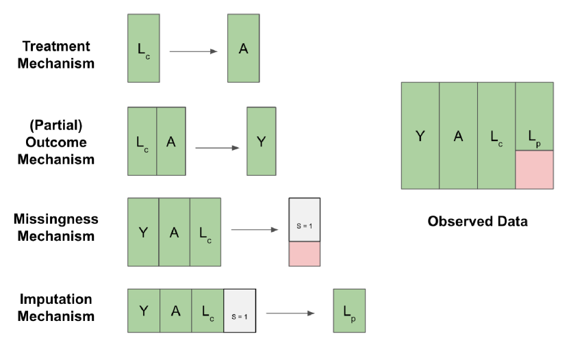
((a)) Levis Factorization

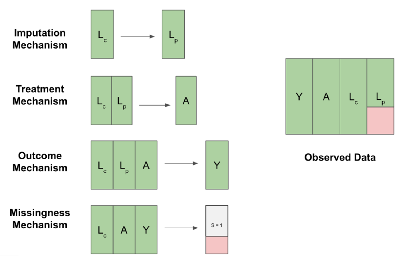
((b)) Alternative Factorization

Figure 2: Two factorizations of the observed data likelihood. While the alternative factorization (shown in panel (b)) may seem more consistent with how data arise temporally, component nuisance models are not directly estimable from the observed data, whereas they are under the “Levis factorization” (shown in panel (a)) from Equation (1).

On the basis of this novel factorization of the observed (coarsened) data likelihood, Levis et al.¹ introduce a complete-case missing at random (CCMAR) assumption, and propose two estimators for the mean counterfactual $\mathbb{E}[Y(a)]$ that are valid under CCMAR. The first is an inverse-weighted outcome regression (IWOR) estimator, $\tilde{\chi}_{a}$, and the second is an influence function-based estimator $\hat{\chi}_{a}$. The influence function-based estimator, $\hat{\chi}_{a}$, is of primary interest as Levis et al.¹ are able to prove several results regarding the robustness and non-parametric efficiency of this estimator. Nevertheless, $\tilde{\chi}_{a}$ serves as a useful comparison point in our simulation study as another estimator derived from the factorization considered in Equation (1). Formal definitions and derivations of $\tilde{\chi}_{a}$ and $\hat{\chi}_{a}$ are presented in $\S 5.1$ and $\S 5.2$ of Levis et al.¹, respectively; for completeness, we give the form of these estimators in the supplementary materials. Henceforth, we will refer to $\tilde{\chi}_{a}$ and $\hat{\chi}_{a}$ as CCMAR-based estimators.

Formally, this complete-case missing at random assumption states that whether or not a patient is a “complete case" depends only on variables observed for all patients. That is,

$$S\perp\!\!\!\perp L_{p}\mid L_{c},A,Y$$ (2)

A noteworthy feature of this particular assumption is that it is agnostic to which components of $L_{p}$ may be missing for any particular subject. That is, this assumption is strictly in regards to whether a subject has complete data $(S=1)$ or not $(S=0)$. Of immediate consequence is that when this assumption holds, estimation strategies for $\tilde{\chi}_{a}$ and $\hat{\chi}_{a}$ do not require estimation or specification of complex, non-monotone missingness patterns that are common in EHR data⁷.

Nuisance Function	Definition	Description	$\tilde{\chi}_{a}$	$\hat{\chi}_{a}$
$\eta(L_{c},a)$	$P_{o^{\prime}}[A=a\leavevmode\nobreak\ |\leavevmode\nobreak\ L_{c}]$	Treatment Mechanism
$\mu(y\leavevmode\nobreak\ |\leavevmode\nobreak\ L_{c},A)$	$P_{o^{\prime}}[Y\leq y\leavevmode\nobreak\ |\leavevmode\nobreak\ L_{c},A]$	Outcome Distribution
$\pi(L_{c},A,Y)$	$P_{o^{\prime}}[S=1\leavevmode\nobreak\ |\leavevmode\nobreak\ L_{c},A,Y]$	Missingness Mechanism
$\lambda(\ell_{p}\leavevmode\nobreak\ |\leavevmode\nobreak\ L_{c},A,Y,S=1)$	$p_{o^{\prime}}[\ell_{p}\leavevmode\nobreak\ |\leavevmode\nobreak\ L_{c},A,Y,S=1]$	Imputation Model

Table 2: Summary of nuisance functions. Checkmarks indicate whether each component must be estimated for the influence function-based estimator $\hat{\chi}_{a}$ and the inverse-weighted outcome regression estimator $\tilde{\chi}_{a}$ from Levis et al.¹

The decomposition in Equation (1) may be considered somewhat unnatural given the temporal order of data occurring in the real world. Typically, when envisioning how data are generated, one first might imagine a process giving rise to any baseline covariates (confounders) of interest, followed by a mechanism for selection into a particular treatment group conditional on those covariates, and finally outcomes are generated conditional on covariates and treatment. Missing data might arise in a number of ways, but one may hypothesize an additional missing at random (MAR) missingness mechanism conditional on treatment, outcome, and observed covariates.

Such a factorization of the observed data likelihood, which we term "alternative factorization" may be expressed as follows.

$$p(O^{\prime})=p(L_{c})\underbrace{p(L_{p}\leavevmode\nobreak\ |\leavevmode\nobreak\ L_{c})^{s}}_{\tilde{\lambda}}\underbrace{p(A\leavevmode\nobreak\ |\leavevmode\nobreak\ L_{c},L_{p})}_{\tilde{\eta}}\underbrace{p(Y\leavevmode\nobreak\ |\leavevmode\nobreak\ L_{c},L_{p},A)}_{\tilde{\mu}}\underbrace{p(S\leavevmode\nobreak\ |\leavevmode\nobreak\ L_{c},A,Y)}_{\pi}$$ (3)

The components of this likelihood are slightly different than those in Equation (1) in that what is being conditioned on is different. Nevertheless, we use similar notation to represent the nuisance functions in this alternative factorization. As shown in Figure 2, component nuisances functions under this factorization are not directly estimable from the observed data due to conditioning on partially observed confounders $L_{p}$.

3 Data Driven Simulation Study

In order to compare the validity of various reasonable but ad hoc analytic approaches in the setting of both missing data and confounding to the CCMAR-based estimators, we conduct a series of simulations. The goals of these simulations are twofold: first, we hope to learn where ad hoc approaches that combine imputation with some method to account for confounding can perform reasonably well, and where they may breakdown; secondly, we hope to learn how the CCMAR-based estimators perform when data are generated by the alternative factorization in Equation (3).

The framing of this simulation study is a hypothetical study comparing two bariatric surgery procedures on long term weight-loss maintenance ². Specifically, let $A$ be a binary point exposure taking on value 0 for Roux-en-Y gastric bypass (RYGB) and 1 for vertical sleeve gastrectomy (VSG). We let $Y$ denote the proportion weight change at 5 years post surgery, relative to baseline. In our simulations we consider up to 5 confounders: gender, baseline BMI at surgery (centered at 30), an indicator of Hispanic ethnicity, baseline Charlson-Elixhauser comorbidity score³⁰, and an indicator of smoking status; we denote these confounders as $(L^{(1)},L^{(2)},L^{(3)},L^{(4)},L^{(5)})$, respectively.

To ensure our simulations reflect plausible real-world settings, simulations are based on data from 5,693 patients who underwent either of the two bariatric procedures of interest at Kaiser Permanente Washington between January 1, 2008 and December 31, 2010. Complete information on gender, baseline BMI, and ethnicity, was available for all patients, while comorbidity scores were only available for 4,344 patients. Smoking status was not measured at all in the data, so we synthetically generated this confounder subject to partial missingness. This was done to create more complex scenarios with multiple partially missing confounders. In all simulation settings, the completely observed confounders were $L_{c}=(L^{(1)},L^{(2)},L^{(3)})$, while the partially observed confounders were either the univariate $L_{p}=L^{(4)}$, or the bivariate $L_{p}=(L^{(4)},L^{(5)})$, depending on the simulation setting.

3.1 Data Generation Process

To specify the "true" components of the likelihood, which were then used to generate simulated datasets, a series of models was fit to the Kaiser Permanente data. Of primary interest was generating data from the novel factorization expressed in Equation (1), and comparing the CCMAR-based estimators using the "true" parametric models, with a suite of approaches described in Section 3.2. Data generation under this factorization is described in Section 3.1.1.

Also of interest was generating a similar comparison of the CCMAR-based estimators with various combinations of imputation and outcome regression or inverse probability weighting, when data were generated from an alternative factorization of the observed data likelihood, described in Section 3.1.2—this alternative factorization is shown visually in Figure 2(b). In this case, the "true" nuisance functions in the factorization proposed by Levis et al.¹ (i.e., those in Table 2) were unknown and would not necessarily be derivable in closed form. As such, results of simulations under this specification can help demonstrate how the CCMAR-based estimators might perform when the true underlying nuisance functions are unknown and need to be modeled and estimated. This, of course, is akin to the problem faced by an analyst in any practical setting.

In each simulation setting considered, 5,000 datasets of size $n=4,344$ patients were generated and analyzed according to the procedures outlined in the remainder of this section. In the main paper we present results from 4 data driven simulations settings, summarized as follows.

1. Factorization in Equation (1), 1 partially missing confounder.

2. Factorization in Equation (1), 1 partially missing confounder, additional non-linearities and interactions in imputation mean model, induced skew in distribution of imputation model.

3. Factorization in Equation (1), 2 partially missing confounders, amplified interactions between $A,L_{p}$, and $Y$ in joint imputation model, induced skew in distribution of imputation model .

4. Alternative factorization, 2 partially missing confounders, amplified interactions between $L_{c},L_{p}$ in full treatment model $\tilde{\eta}(L_{c},L_{p},a)$.

Results from an additional 15 data-driven simulation settings are available in the supplementary materials.

3.1.1 Factorization in Equation (1)

To inform simulated datasets under Equation (1), each of the 4 nuisance functions for this factorization of the observed data likelihood, outlined in Table 2, were modeled by fitting regression models to the Kaiser Permanente data. These models were used to help specify the "true" components of the likelihood. Specifically, logistic regressions were fit for $\eta$ and $\pi$, and a Gaussian linear model was fit for $\mu$. In the Kaiser Permanente data, the comorbidity score $(L^{(4)}=L_{p1})$ is categorical, but we instead chose to fit a generalized linear model with gamma link function to make the underlying relationship more complex. In fact, numerical integration techniques such as Gaussian quadrature are required to compute $\hat{\chi}_{a}$ when $L_{p}$ contains continuous confounders.

In certain simulation settings, we simulated a second missing confounder, smoking status $(L^{(5)}=L_{p2})$ from a logistic regression model with pre-specifed effect sizes given that no such smoker indicator is available in the Kaiser Permanente data. Such generation follows from the decomposition of the joint density of $L_{p}$ as follows

$$\lambda(\ell_{p1},\ell_{p2}\leavevmode\nobreak\ |\leavevmode\nobreak\ L_{c},A,Y,S=1)=\lambda_{1}(\ell_{p1}\leavevmode\nobreak\ |\leavevmode\nobreak\ L_{c},A,Y,S=1)\lambda_{2}(\ell_{p2}\leavevmode\nobreak\ |\leavevmode\nobreak\ L_{c},A,Y,S=1,L_{p1}=\ell_{p1})$$ (4)

where $\lambda_{1}$ and $\lambda_{2}$ represent the conditional densities of the 2 confounders in $L_{p}$, corresponding to $L^{(4)}$ and $L^{(5)}$, respectively.

In each simulation, $L_{c,1}...L_{c,n}$ were drawn with replacement from the empirical values in the Kaiser Permanente data. Then, $(A_{i},Y_{i},S_{i},S_{i}L_{p,i})$ for $i=1,...,n$ were independently sampled, sequentially, from the following models, with covariates ($X$) and coefficients ($\beta$) for each model simulations available in Table 3.

• $\text{logit}(\eta(L_{c},1))=\text{logit}(P[A=1\leavevmode\nobreak\ |\leavevmode\nobreak\ L_{c}])=\beta_{\eta}^{T}X_{\eta}$

• $Y\leavevmode\nobreak\ |\leavevmode\nobreak\ L_{c},A\sim\mathcal{N}(\beta_{\mu}^{T}X_{\mu},\sigma^{2}_{Y})$

• $\text{logit}(\pi(L_{c},A,Y))=\text{logit}(P[S=1\leavevmode\nobreak\ |\leavevmode\nobreak\ L_{c},A,Y])=\beta_{\pi}^{T}X_{\pi}$

• $L_{p1}\leavevmode\nobreak\ |\leavevmode\nobreak\ L_{c},A,Y,S=1\sim\text{Gamma}(\alpha,\lambda_{1}(L_{c},A,Y))$ with rate parameter $\lambda_{1}(L_{c},A,Y)=\frac{\alpha}{\mathbb{E}[L_{p1}\leavevmode\nobreak\ |\leavevmode\nobreak\ L_{c},A,Y,S=1]}$, and we parameterize $\log(\mathbb{E}[L_{p1}\leavevmode\nobreak\ |\leavevmode\nobreak\ L_{c},A,Y,S=1])=\beta_{\lambda_{1}}^{T}X_{\lambda_{1}}$

• $\text{logit}(\lambda_{2}(L_{c},L_{p1},A,Y,S=1))=\text{logit}(P[L_{p2}=1\leavevmode\nobreak\ |\leavevmode\nobreak\ L_{c},L_{p1},A,Y,S=1])=\beta_{\lambda_{2}}^{T}X_{\lambda_{2}}$ (for simulations with multiple partially missing confounders).

We considered several settings where certain effects in the 4 nuisance models were amplified in order to create more interesting and complex relationships across confounders, treatment and outcome.

3.1.2 Alternative Factorization

Since it is of interest to assess the performance of CCMAR-based estimators where the "true" nuisance functions are unknown (and perhaps not derivable in closed form), we considered an additional data generating process based on Equation (3) which reflects the more "natural" order described in the previous section. In simulations with multiple missing confounders, the joint density of $L_{p}$ decomposes as follows:

$$\tilde{\lambda}(\ell_{p1},\ell_{p2}\leavevmode\nobreak\ |\leavevmode\nobreak\ L_{c})=\tilde{\lambda}_{1}(\ell_{p1}\leavevmode\nobreak\ |\leavevmode\nobreak\ L_{c},)\tilde{\lambda}_{2}(\ell_{p2}\leavevmode\nobreak\ |\leavevmode\nobreak\ L_{c},L_{p1}=\ell_{p1})$$ (5)

where $\tilde{\lambda}_{1}$ and $\tilde{\lambda}_{2}$ represent the conditional densities of the 2 confounders in $L_{p}$, corresponding to $L^{(4)}$ and $L^{(5)}$, respectively.

Similar to the data-driven strategy described in Section 3.1.1, for simulating datasets under Equation (3), each of the 4 nuisance functions for the alternative factorization of the observed data likelihood were fit to the Kaiser Permanente data to specify the "true" components of the likelihood. In fact, the type of parametric models used to fit these nuisance models under the alternative factorization were the same as under the previous factorization: logistic regressions were fit for $\tilde{\eta}$ and $\pi$, a Gaussian linear model was fit for $\tilde{\mu}$, a generalized linear model with gamma link function for $\tilde{\lambda}_{1}$ and a logistic regression for $\tilde{\lambda}_{2}$. The key differences between the models used to inform the truth in the previous factorization versus the alternative factorization are the sets of variables included in the relevant conditioning sets, i.e., what covariates can be conditioned on.

In each simulation, $L_{c,1}...L_{c,n}$ were drawn with replacement from the empirical values from the Kaiser Permanente data. Then $(L_{p,i},A_{i},Y_{i},S_{i})$ for $i=1,...,n$ were independently sampled, sequentially, from the following models.

• $L_{p1}\leavevmode\nobreak\ |\leavevmode\nobreak\ L_{c}\sim\text{Gamma}(\alpha,\lambda_{1}(L_{c}))$ with rate parameter $\lambda_{1}(L_{c})=\frac{\alpha}{\mathbb{E}[L_{p1}\leavevmode\nobreak\ |\leavevmode\nobreak\ L_{c}]}$, and we parameterize $\log(\mathbb{E}[L_{p1}\leavevmode\nobreak\ |\leavevmode\nobreak\ L_{c}])=\beta_{\lambda_{1}}^{T}X_{\lambda_{1}}$

• $\text{logit}(\lambda_{2}(L_{c},L_{p1}))=\text{logit}(P[L_{p2}=1\leavevmode\nobreak\ |\leavevmode\nobreak\ L_{c},L_{p1}])=\beta_{\lambda_{2}}^{T}X_{\lambda_{2}}$ (for simulations with multiple partially missing confounders).

• $\text{logit}(\eta(L_{c},L_{p},1))=\text{logit}(P[A=1\leavevmode\nobreak\ |\leavevmode\nobreak\ L_{c},L_{p}])=\beta_{\eta}^{T}X_{\eta}$

• $Y\leavevmode\nobreak\ |\leavevmode\nobreak\ L_{c},L_{p},A\sim\mathcal{N}(\beta_{\mu}^{T}X_{\mu},\sigma^{2}_{Y})$

• $\text{logit}(\pi(L_{c},A,Y))=\text{logit}(P[S=1\leavevmode\nobreak\ |\leavevmode\nobreak\ L_{c},A,Y])=\beta_{\pi}^{T}X_{\pi}$

Note that even though $L_{p}$ was generated when $S=0$, we ignore this information and artificially set the observed data to be $(L_{c},A,Y,S,SL_{p})$, as before. We considered several settings where certain effects in the 4 nuisance models were amplified in order to create more interesting and complex relationships across confounders, treatment and outcome. Covariates ($X$) and coefficients ($\beta$) for each model are presented in Table 3.

		Data Driven Simulation Scenario
Model	Term	1	2	3	4
	(Intercept)	-0.624	-0.624	-0.624	-0.586
	$L^{(1)}$	0.308	0.308	0.308	0.311
	$L^{(2)}$	-0.046	-0.046	-0.046	-0.046
	$L^{(3)}$	-0.015	0.385	0.385	0.384
	$L^{(4)}$	—	—	—	-0.035
	$(L^{(2)})^{2}$	0.001	0.001	0.001	0.001
	$L^{(1)}\times L^{(3)}$	0.400	0.400	0.400	0.100
$\eta$ or $\tilde{\eta}$	$L^{(3)}\times L^{(4)}$	—	—	—	-0.020
	(Intercept)	-0.207	-0.207	-0.207	-0.200
	$L^{(1)}$	0.031	0.031	0.031	0.032
	$L^{(2)}$	-0.002	-0.002	-0.002	-0.002
	$L^{(3)}$	0.023	0.023	0.023	0.022
	$L^{(4)}$	—	—	—	-0.004
	$L^{(5)}$	—	—	—	0.200
	$L^{(1)}\times L^{(3)}$	-0.305	-0.305	-0.305	-0.305
	$L^{(4)}\times L^{(5)}$	—	—	—	-0.001
	$A$	0.045	0.045	0.045	0.047
	$A\times L^{(1)}$	0.413	0.313	0.313	0.313
	$A\times L^{(2)}$	-0.003	-0.001	-0.001	0.005
	$A\times L^{(3)}$	0.130	0.080	0.080	0.081
	$A\times L^{(4)}$	—	—	—	-0.002
	$A\times L^{(5)}$	—	—	—	0.100
$\mu$ or $\tilde{\mu}$	$\sigma$	0.109	0.109	0.109	0.109
	(Intercept)	1.824	1.824	1.824	1.824
	$L^{(1)}$	0.087	0.087	0.087	0.087
	$L^{(2)}$	0.010	0.010	0.010	0.010
	$L^{(3)}$	-2.662	-2.662	-2.662	-2.662
	$L^{(2)}\times L^{(3)}$	-0.149	-0.149	-0.149	-0.149
	$A$	2.922	2.922	2.922	2.922
	$Y$	2.180	2.180	2.180	2.180
	$A\times Y$	3.043	3.043	3.043	3.043
	$A\times L^{(2)}$	0.159	0.159	0.159	0.159
$\pi$	$Y\times L^{(1)}$	2.321	2.321	2.321	2.321

		Data Driven Simulation Scenario
Model	Term	1	2	3	4
	(Intercept)	0.867	0.939	0.939	0.900
	$L^{(1)}$	0.075	0.074	0.074	0.272
	$L^{(2)}$	< 0.001	-0.018	-0.018	0.001
	$L^{(3)}$	-0.034	-0.033	-0.033	-0.035
	$(L^{(2)})^{2}$	—	< 0.001	< 0.001	—
	$L^{(1)}\times L^{(2)}$	—	—	—	0.001
	$L^{(1)}\times L^{(3)}$	—	—	—	0.100
	$A$	0.303	0.102	0.302	—
	$Y$	-0.765	-0.696	-0.696	—
	$A\times Y$	-0.500	-0.050	-0.500	—
	$Y\times L^{(2)}$	—	-0.005	-0.005	—
$\lambda_{1}$ or $\tilde{\lambda}_{1}$	$\alpha$	3.619	1.000	1.000	3.616
	(Intercept)	—	—	-1.386	-1.386
	$L^{(1)}$	—	—	—	0.030
	$L^{(2)}$	—	—	—	0.050
	$L^{(3)}$	—	—	—	0.025
	$L^{(4)}$	—	—	0.075	0.075
	$A$	—	—	—	—
	$Y$	—	—	-4.000	—
	$A\times Y$	—	—	2.000	—
	$A\times L^{(4)}$	—	—	-0.010	—
	$Y\times L^{(2)}$	—	—	—	—
$\lambda_{2}$ or $\tilde{\lambda}_{2}$	$Y\times L^{(4)}$	—	—	0.010	—

Table 3: Coefficients ($\beta$) and covariates ($X$) used to generated simulated datasets for each of the four simulation scenarios presented in the main paper. Scenarios 1-3 generated datasets using the Levis factorization (Equation (1)), while scenario 4 generated datasets using an alternative factorization (Equation (3)). — denotes the given covariate was not including in the corresponding model. Note that simulation scenarios 1-2 only generated a single partially missing confounder and as such no $\lambda_{2}$ model was needed.

3.2 Methods

Across our simulation settings, we considered combinations of several methods for imputation of $L_{p}$ in conjunction with the use of outcome regression or inverse probability weighting to address the issue of confounding. Specifically, we considered methods that vary in both model flexibility (parametric, semi-parametric, non-parametric) and structure (interactions vs. no interactions).

We considered 3 imputation models for $L_{p}$: the correctly specified data generating process for $L_{p}$ (a gamma generalized linear model for comorbidity score $(L^{(4)})$ and a logistic regression for smoking status $(L^{(5)})$, with exact models depending on the corresponding factorization under which data were generated); a simpler imputation model with a Gaussian linear model for comorbidity score and a logistic regression for smoking status, with neither model considering any interactions; and, an imputation model with a Gaussian linear model for comorbidity score and a logistic regression for smoking status, while specifying all pairwise interactions. To avoid overfitting/variance inflation due to specifying all pairwise interactions, linear/logistic regression models in this third case were fit using glmnet³¹ in R with $L_{1}$ (LASSO)³² regularization. Additionally, we considered a fourth strategy where the problem of missing data was ignored and subjects with missing these data were dropped, in order to mimic a complete case analysis.

Upon imputing (or not imputing) $L_{p}$, we considered several methods to directly model $Y$ in order to estimate the mean counterfactual outcome $\mathbb{E}[Y^{(a)}]$ using outcome regression. In particular, we considered 3 types of models ranging in flexibility: linear regression, with no interactions and with all pairwise interactions specified; generalized additive models (GAMs)³³, with no interactions and with all pairwise interactions specified; and random forest. As was the case with the linear regression models used for imputation of $L_{p}$, outcome regression models specifying all pairwise interactions were estimated with glmnet³¹ using $L_{1}$ (LASSO)³² regularization.

In the case of GAMs, interactions took on one of three forms. When two covariates were binary, interaction effects were simply the coefficient for product of the covariates, as in a linear regression model. For covariates $x_{1}\in\{0,1\},x_{2}\in\mathbb{R}$, interaction effects were the coefficients for the product $x_{1}f(x_{2})$, where $f$ is some smooth basis function. Finally, when both covariates were continuous, interaction effects were coefficients for the two dimensional surface $g(x_{1},x_{2})$. In our fitting of GAMs, $f$ was chosen to be a cubic regression spline, while $g$ was a tensor product smoother. Inherent to the fitting of these smooth functions is regularization in the form of choice of degree and/or knots³⁴. Finally, we considered an even more flexible non-parametric random forest model, which can capture complex, highly non-linear relationships between confounders, treatment and outcome.

We employed a similar suite of approaches for IPW as we did for outcome regression, instead modeling the probability of treatment using several models varying in complexity and flexibility. The analogue of the linear regression (with and without interaction effects) when modeling propensity scores was logistic regression, while GAMs with logit link (i.e., GAM logistic regression) were used as the analogue of GAM outcome regression. Random forests were also applied under classification specification to most flexibly model the treatment mechanism. Table 4 summarizes the suite of "standard" models—in line with the alternative factorization—considered in simulations for comparison against the CCMAR-based estimators.

When computing the CCMAR-based estimators, we used correctly specified parametric models for simulated datasets generated under the factorization of Equation (1) (scenarios 1–3). Under the alternative factorization (scenario 4), we fit the same parametric models used in scenarios 1-3, as well as flexible versions of the estimators which used GAMs with logit link for $\hat{\eta}$, $\hat{\pi}$ and $\hat{\lambda}_{2}$, a traditional GAM for $\hat{\mu}$, and a GAM with underlying gamma distribution for $\hat{\lambda}_{1}$. In this flexible version of the CCMAR-based estimators, GAMs include all pairwise interactions. We also considered a version of the CCMAR-based estimators with a GAM with underlying Gaussian distribution for $\hat{\lambda}_{1}$.

Imputation of $L_{p}$
Imputation Process	Confounder	Model Type	Covariates	Interactions
True Data Generating Process	$L^{(4)}$	Gamma GLM	$A,Y,L_{c}$	When Applicable
	$L^{(5)}$	Logistic Regression	$A,Y,L_{c},L^{(4)}$	When Applicable
Simple Imputation	$L^{(4)}$	Linear Regression	$A,Y,L_{c}$	—
	$L^{(5)}$	Logistic Regression	$A,Y,L_{c},L^{(4)}$	—
Imputation w/ Interactions	$L^{(4)}$	Linear Regression	$A,Y,L_{c}$	All Pairwise∗
	$L^{(5)}$	Logistic Regression	$A,Y,L_{c},L^{(4)}$	All Pairwise∗
No Imputation (Complete Case)	$L^{(4)}$	—	—	—
	$L^{(5)}$	—	—	—
Outcome Regression Model
Model Type		Covariates	Imputed Datasets Used	Interactions
Linear Regression		$A,L_{c},L_{p}$	All	—
				All Pairwise∗
Generalized Additive Models		$A,L_{c},L_{p}$	All	—
				All Pairwise
Random Forest		$A,L_{c},L_{p}$	All	Implicit in model
Probability of Treatment Model (IPW)
Model Type		Covariates	Imputed Datasets Used	Interactions
Logistic Regression		$L_{c},L_{p}$	All	—
				All Pairwise∗
Generalized Additive Models (Logistic Regression)		$L_{c},L_{p}$	All	—
				All Pairwise
Random Forest		$L_{c},L_{p}$	All	Implicit in model

LASSO^{32, 31} regularization in model with pairwise interactions specified in order to select meaningful interaction effects.

Table 4: Summary of approaches in simulation settings combining imputation with one of two methods for accounting for confounding (outcome regression or IPW). First, partially missing confounders $L_{p}$ are imputed using one of 3 techniques, or alternatively subjects missing these data are dropped to mimic a complete case analysis. Various types of models ranging in flexibility—both in terms of types of interactions included as well as the structure of the model—are estimated to model either the outcome or probability of treatment in order to estimate mean counterfactual outcomes $\mathbb{E}[Y^{(a)}]$ in a manner that addresses confounding.

4 Simulation Study with Non-Parametric Nuisance Models

The suite of simulation scenarios based on our running bariatric surgery example in Section 3 does not consider the performance of the CCMAR-based estimators of Levis et al.¹ using fully non-parametric model choices for the nuisance functions. In data driven simulation scenario 4, GAMs were used to flexibly model the mean parameter in each nuisance model, but GAMs still make distributional assumptions for the residuals (e.g. Gamma or Gaussian). In order to evaluate the performance of these new estimators in a fully flexible manner, we designed an additional, small scope simulation study based on the worked data example described in Levis et al.¹, which utilized a fully non-parametric approach. Due to computational overhead associated with non-parametric conditional density estimation, and subsequent numerical integration over such densities, this simulation study is somewhat simpler than those presented in the previous section. Nevertheless, the presence of multiple missing confounders make it sufficiently challenging to gain insight into the performance of Levis et al.’s estimators in their most flexible form.

4.1 Data Generation Process

In this simulation $L_{c}=\emptyset$ and $L_{p}=(L_{p1},L_{p2})$, where $L_{p1}$ is a binary covariate and $L_{p2}$ is a continuous covariate. For 1,000 replicates of size $n=5,000$ subjects, i.i.d. copies of $(A_{i},Y_{i},S_{i},SL_{p,i})$ were generated as follows:

$$A \sim\text{Bernoulli}(0.5)$$

$$Y\leavevmode\nobreak\ |\leavevmode\nobreak\ A \sim\begin{cases}\text{Beta}(2,4)&\text{if}\leavevmode\nobreak\ A=0\\ \text{Beta}(4,2)&\text{if}\leavevmode\nobreak\ A=1\end{cases}$$

$$\text{logit}(P[S=1\leavevmode\nobreak\ |\leavevmode\nobreak\ A,Y]) =-0.35+0.5A+0.18Y+0.05A\times Y$$

$$\text{logit}(P[L_{p1}=1\leavevmode\nobreak\ |\leavevmode\nobreak\ A,Y,S=1]) =-0.6+0.5A+0.25Y+0.1A\times Y$$

$$L_{p2}\leavevmode\nobreak\ |\leavevmode\nobreak\ A,Y,S=1,L_{p1} \sim\mathcal{N}(A+Y+2.5L_{p1}\times Y,1.25^{2})$$

4.2 Methods

The CCMAR-based estimators were computed using non-parametric methods for each nuisance function, as well as, for comparison, the correctly specified parametric nuisance functions. In the case of non-parametric estimation, $\hat{\eta}(0)=\hat{\eta}(1)=0.5$, essentially assuming treatment assignment probabilities were known by design. The conditional density of $Y$ given $A$, $d\hat{\mu}$ was fit using the highly adaptive lasso conditional density estimator³⁵ in the haldensify R package ^{36, 37}, with 25 equally sized bins and maximum degree of basis function interaction of 3. Probability of missingness $\hat{\pi}(A,Y)$ was estimated with an ensemble regression learner from the SuperLearner package in R^{38, 39}. Component models in the ensemble included a generalized linear model with all second order interactions, as well as multivariate adaptive polynomial spline regressions⁴⁰. The probability mass function of the binary covariate $L_{p1}$, $\hat{\lambda}_{1}(\ell_{p1}\leavevmode\nobreak\ |\leavevmode\nobreak\ A,Y)$, was estimated via the same SuperLearner ensembling strategy. Finally, the conditional density of the continuous partially observed covariate $\hat{\lambda}_{2}(\ell_{p2}\leavevmode\nobreak\ |\leavevmode\nobreak\ A,Y,\ell_{p1})$ was estimated using the same highly adaptive lasso conditional density estimator that was used for estimating $d\hat{\mu}$.

Due to the non-parametric nature of the nuisance function models, the CCMAR-based estimators were computed via 2-fold cross fitting^{41, 42, 43}. Briefly, this involved splitting each simulated data set into two equally sized partitions, using one to fit the nuisance models and the other to compute the estimator on the basis of the estimated nuisance functions. The roles of the two folds were then swapped and the results from each fold were averaged to produce a final estimator per dataset.

5 Results

Results from the 4 most pertinent simulation scenarios based on the bariatric surgery example are presented in Tables 5–8. Results examining the properties of the fully non-parametric CCMAR-based estimators are presented in Table 9. Expanded results from an additional 15 data driven simulation scenarios are available in our supplementary materials. We summarize several key findings and observations as follows:

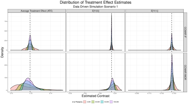
Figure 3: Distribution of estimated treatment effects under simulation scenario 1 using the complete-case missing at random (CCMAR) influence function-based (IF) and inverse-weighted outcome regression (IWOR) estimators. 5,000 simulated datasets where generated for each number of patients, $n$. For every contrast, the IWOR estimator does tend toward asymptotically normal, but its empirical rate of convergence appears to be much slower than the IF based estimator. This behavior is likely what gives rise to the larger median bias observed in the IWOR estimator, despite the mean having little to no bias in most scenarios.

Data Driven Simulation Scenario 1
Model		Interactions	Imputation	% Bias	% M-Bias	SE	Relative Uncertainty
	IF		—	0	0	0.006	1.000
CCMAR-based	IWOR	—	—	-1	-6	0.029	5.088
			OLS/LR	15	15	0.006	1.005
			OLS/LR w/ Interactions	12	12	0.006	1.015
			True DGP	14	14	0.006	1.005
		None	—	-21	-21	0.006	1.049
			OLS/LR	0	0	0.005	0.812
			OLS/LR w/ Interactions	0	0	0.005	0.824
			True DGP	0	0	0.005	0.813
	OLS	Pairwise	—	-24	-24	0.006	0.973
			OLS/LR	15	15	0.006	1.007
			OLS/LR w/ Interactions	12	12	0.006	1.011
			True DGP	14	14	0.006	1.006
		None	—	-21	-21	0.006	1.050
			OLS/LR	0	0	0.005	0.846
			OLS/LR w/ Interactions	0	0	0.005	0.848
			True DGP	0	0	0.005	0.821
	GAM	Pairwise	—	-23	-23	0.006	0.982
			OLS/LR	-1	-1	0.005	0.836
			OLS/LR w/ Interactions	-1	-1	0.005	0.835
			True DGP	-1	-1	0.005	0.831
Outcome Regression	Random Forest	—	—	-30	-30	0.006	1.008
			OLS/LR	8	8	0.006	0.959
			OLS/LR w/ Interactions	6	6	0.006	0.958
			True DGP	8	8	0.006	0.965
		None	—	-22	-22	0.007	1.175
			OLS/LR	0	0	0.005	0.857
			OLS/LR w/ Interactions	0	0	0.005	0.886
			True DGP	1	1	0.005	0.865
	Logistic Regression	Pairwise	—	-26	-26	0.007	1.203
			OLS/LR	6	6	0.006	1.003
			OLS/LR w/ Interactions	4	4	0.006	0.988
			True DGP	7	7	0.006	0.956
		None	—	-23	-23	0.007	1.174
			OLS/LR	0	-1	0.005	0.895
			OLS/LR w/ Interactions	0	0	0.005	0.934
			True DGP	1	1	0.005	0.839
	GAM (Logit Link)	Pairwise	—	-26	-26	0.007	1.250
			OLS/LR	-1	-1	0.005	0.896
			OLS/LR w/ Interactions	-1	-1	0.005	0.903
			True DGP	1	1	0.005	0.904
IPW	Random Forest	—	—	-24	-24	0.006	0.959
IF = Influence Function; IWOR = Inverse-Weighted Outcome Regression
% Bias = 100 $\times$ Relative Bias of Mean Average Treatment Effect Estimate
% M-Bias = 100 $\times$ Relative Bias of Median Average Treatment Effect Estimate
Relative Uncertainty = Ratio of standard error to standard error of CCMAR-based IF Estimator
Imputation: Linear Regression (OLS), Logistic Regression (LR), True Data Generating Process (DGP)

Table 5: Data Driven Simulation Scenario # 1: Factorization in Equation (1), 1 partially missing confounder.

Data Driven Simulation Scenario 2
Model		Interactions	Imputation	% Bias	% M-Bias	SE	Relative Uncertainty
	IF		—	0	0	0.004	1.000
CCMAR-based	IWOR	—	—	-1	-5	0.020	4.587
			OLS/LR	5	5	0.005	1.100
			OLS/LR w/ Interactions	5	5	0.005	1.099
			True DGP	5	5	0.005	1.099
		None	—	-23	-23	0.005	1.235
			OLS/LR	0	-1	0.004	0.947
			OLS/LR w/ Interactions	-1	-1	0.004	0.947
			True DGP	0	0	0.004	0.948
	OLS	Pairwise	—	-19	-19	0.005	1.207
			OLS/LR	4	4	0.005	1.113
			OLS/LR w/ Interactions	4	4	0.005	1.115
			True DGP	5	5	0.005	1.100
		None	—	-23	-23	0.005	1.237
			OLS/LR	-1	-1	0.004	0.989
			OLS/LR w/ Interactions	-1	-1	0.004	0.991
			True DGP	0	0	0.004	0.948
	GAM	Pairwise	—	-18	-18	0.005	1.215
			OLS/LR	-1	-1	0.004	0.974
			OLS/LR w/ Interactions	-1	-2	0.004	0.977
			True DGP	0	0	0.004	0.960
Outcome Regression	Random Forest	—	—	-25	-25	0.006	1.267
			OLS/LR	-4	-4	0.005	1.048
			OLS/LR w/ Interactions	-4	-4	0.005	1.046
			True DGP	-4	-4	0.005	1.048
		None	—	-26	-26	0.006	1.262
			OLS/LR	0	0	0.004	0.955
			OLS/LR w/ Interactions	0	0	0.004	0.960
			True DGP	0	0	0.004	0.956
	Logistic Regression	Pairwise	—	-22	-23	0.006	1.356
			OLS/LR	-6	-6	0.006	1.320
			OLS/LR w/ Interactions	-6	-6	0.006	1.402
			True DGP	-4	-4	0.005	1.043
		None	—	-26	-26	0.006	1.267
			OLS/LR	-2	-2	0.005	1.129
			OLS/LR w/ Interactions	-2	-2	0.005	1.177
			True DGP	0	0	0.004	0.954
	GAM (Logit Link)	Pairwise	—	-22	-22	0.007	1.577
			OLS/LR	-3	-3	0.004	0.990
			OLS/LR w/ Interactions	-3	-3	0.004	0.993
			True DGP	0	0	0.004	0.984
IPW	Random Forest	—	—	-21	-21	0.005	1.108
IF = Influence Function; IWOR = Inverse-Weighted Outcome Regression
% Bias = 100 $\times$ Relative Bias of Mean Average Treatment Effect Estimate
% M-Bias = 100 $\times$ Relative Bias of Median Average Treatment Effect Estimate
Relative Uncertainty = Ratio of standard error to standard error of CCMAR-based IF Estimator
Imputation: Linear Regression (OLS), Logistic Regression (LR), True Data Generating Process (DGP)

Table 6: Data Driven Simulation Scenario # 2: Factorization in Equation (1), 1 partially missing confounder, additional non-linearities and interactions in imputation mean model,induced skew in distribution of imputation model.

1. Complete case analysis can be severely biased: In every scenario considered, dropping subjects with missing values for some of the confounders lead to relative bias on the order of magnitude of 20%. This held regardless of whether outcome regression or inverse probability weighting methods were employed, whether flexible models were used, and whether interactions were included in the models.

1. Sufficient model flexibility can overcome confounding bias due to model misspecification: As seen in scenario 1, adding pairwise interactions to outcome regression models (OLS and GAM) or propensity score models (logistic regression, GAM logistic regression) removed bias observed when such terms were omitted. Similarly, random forest models for either the outcome or propensity score yielded results with very small bias.

1. Flexibility does not always come at the expense of efficiency: In the majority of scenarios considered, the relative uncertainty of methods not including interactions exceeded 1, indicating estimators were less efficient than the influence function CCMAR-based estimator. In fact, including pairwise interaction terms frequently improved estimator efficiency. In many scenarios, such as # 1-2, the inclusion of pairwise interactions pushed relative uncertainty below 1, indicating estimators were more efficient than the influence function CCMAR-based estimator. Additionally, non-parametric random forest methods consistently displayed some of the best efficiency metrics observed across scenarios. Thus, perhaps somewhat counter to common intuition, efficiency is not always lost when increasing model flexibility.

1. Model flexibility does not guarantee unbiasedness: Deploying flexible models, like GAMs, without interactions yielded bias in both directions depending on the simulation scenario and analysis method (IPW versus outcome regression). In fact, without the inclusion of interactions, flexible models like GAM did no better than simple OLS. This may be because with cubic regression splines, GAMs may regularize many terms to first order anyway. Additionally, GAMs can account for non-linearities but does not inherently account for interactions unless such terms are specified. Similarly, even fully non-parametric models such as random forests, which can account for both non-linearities and complex interactions in predictors, yielded non-trivial bias in scenarios 2-4.

1. Imputation method less important when Normal distribution approximates $\lambda_{1}$ well: In scenario 1, where the single partially missing confounder followed a gamma distribution, there is hardly any difference in bias/efficiency of standard methods across imputation methods. That is, Gaussian linear regression, with or without interactions, seems to impute $L^{(4)}$ sufficiently well such that analysis of corresponding datasets yields results very similar to analysis of datasets where $L^{(4)}$ was imputed using the true gamma data generating process. In scenario 1, the Gamma shape parameter of $\alpha=3.619$ implies that the distribution of $L^{(4)}$ is not too skewed and can be decently approximated by a Normal distribution. However, in scenarios 2-3 where $\alpha=1$ was selected to induce additional skew in the distribution of $L^{(4)}$, unbiased results only arise when the imputation process is in line with the true data generating process, based on the correctly specified Gamma distribution.

1. Standard methods perform well even with multiple missing confounders and amplified relationships: Many of the same patterns emerge in more complex scenarios (e.g., #3) where there are multiple partially missing confounders as well as amplified interaction effects between $A,Y$ and $L_{p}$. Namely:

   • Methods using linear/logistic regressions and GAMs have some bias when interaction terms are not specified.

   • Bias is attenuated when specifying interaction terms in methods using linear/logistic regressions and GAMs.

   • Efficiency tends to improve when including interaction terms.

   • Most methods have relative uncertainty $<1$ (better than influence function CCMAR-based estimator).

   • There exist scenarios where every method is slightly biased unless true data generating process is used for imputation (scenario #3).

1. Influence function CCMAR-based estimator can be biased when nuisance functions misspecified: Under the alternative data generating processes (scenario #4) the CCMAR-based estimators are biased when (incorrect) parametric models are used to estimate nuisance functions. In scenario 4, the majority of standard methods also are biased to varying degrees, as their nuisance model specifications may also be incorrect, but the influence function CCMAR-based estimator has relative bias greater than any standard method outside of complete case analyses.

1. Influence function CCMAR-based estimation with flexible modeling of nuisance functions can overcome bias due to misspecification: In scenario 4, the flexible version of the influence function CCMAR-based estimator, with semi-parametric (GAM) specification of nuisance functions yielded nearly unbiased estimation of the average treatment effect. Flexibly modeling the nuisance functions in Equation (1) fully addressed the bias observed from the parametric specification of the influence function CCMAR-based estimator. Furthermore, as seen in Table 9, this estimator with fully non-parametric nuisance models achieved unbiased results, demonstrating the success of this estimator even in the absence of any knowledge about the true data generating process.

1. The IWOR CCMAR-based estimator is skewed and has poor relative uncertainty: In most scenarios, the CCMAR-based inverse-weighted outcome regression (IWOR) estimator has non-trivial relative bias in the median, even if the mean is unbiased. This skewness can be seen in Figure 3, and compared to the influence function-based estimator, convergence to asymptotic normality empirically seems to happen at a much slower rate. This slower rate of convergence is likely also what leads to biased results in the IWOR estimator when all component nuisance models are non-parametrically specified (Table 9), and speaks to the necessity of the influence function based estimator when pursuing a fully flexible approach.

Data Driven Simulation Scenario 3
Model		Interactions	Imputation	% Bias	% M-Bias	SE	Relative Uncertainty
	IF		—	0	0	0.007	1.000
CCMAR-based	IWOR	—	—	-1	-5	0.020	2.983
			OLS/LR	4	4	0.005	0.759
			OLS/LR w/ Interactions	3	3	0.005	0.753
			True DGP	3	3	0.005	0.745
		None	—	-22	-23	0.006	0.825
			OLS/LR	0	0	0.004	0.650
			OLS/LR w/ Interactions	0	0	0.004	0.646
			True DGP	0	0	0.004	0.645
	OLS	Pairwise	—	-19	-19	0.005	0.804
			OLS/LR	3	3	0.005	0.767
			OLS/LR w/ Interactions	2	2	0.005	0.769
			True DGP	3	3	0.005	0.745
		None	—	-22	-23	0.006	0.826
			OLS/LR	-1	-1	0.005	0.717
			OLS/LR w/ Interactions	-1	-1	0.005	0.695
			True DGP	0	0	0.004	0.644
	GAM	Pairwise	—	-18	-18	0.005	0.811
			OLS/LR	-2	-2	0.004	0.662
			OLS/LR w/ Interactions	-2	-2	0.004	0.661
			True DGP	-1	-1	0.004	0.650
Outcome Regression	Random Forest	—	—	-26	-26	0.005	0.811
			OLS/LR	-5	-5	0.005	0.744
			OLS/LR w/ Interactions	-5	-5	0.005	0.728
			True DGP	-5	-5	0.005	0.727
		None	—	-26	-26	0.006	0.893
			OLS/LR	1	1	0.004	0.658
			OLS/LR w/ Interactions	1	1	0.004	0.658
			True DGP	1	1	0.004	0.655
	Logistic Regression	Pairwise	—	-22	-22	0.006	0.903
			OLS/LR	-7	-7	0.006	0.965
			OLS/LR w/ Interactions	-7	-7	0.007	1.007
			True DGP	-5	-5	0.005	0.723
		None	—	-26	-26	0.006	0.879
			OLS/LR	-1	-1	0.005	0.818
			OLS/LR w/ Interactions	-1	-1	0.006	0.846
			True DGP	1	1	0.004	0.656
	GAM (Logit Link)	Pairwise	—	-22	-22	0.007	1.035
			OLS/LR	-2	-2	0.005	0.671
			OLS/LR w/ Interactions	-2	-2	0.004	0.668
			True DGP	0	0	0.004	0.667
IPW	Random Forest	—	—	-19	-19	0.005	0.747
IF = Influence Function; IWOR = Inverse-Weighted Outcome Regression
% Bias = 100 $\times$ Relative Bias of Mean Average Treatment Effect Estimate
% M-Bias = 100 $\times$ Relative Bias of Median Average Treatment Effect Estimate
Relative Uncertainty = Ratio of standard error to standard error of CCMAR-based IF Estimator
Imputation: Linear Regression (OLS), Logistic Regression (LR), True Data Generating Process (DGP)

Table 7: Data Driven Simulation Scenario $\#3$: Factorization in Equation (1), 2 partially missing confounders, amplified interactions between $A,L_{p}$, and $Y$ in joint imputation model, induced skew in distribution of imputation model.

Data Driven Simulation Scenario 4
Model		Interactions	Imputation	% Bias	% M-Bias	SE	Relative Uncertainty
	IF∗		—	8	2	0.045	1.000
CCMAR-based	IWOR		—	-2	-5	0.024	0.534
	IF†		—	1	1	0.016	0.349
Flexible CCMAR (Gamma $\lambda_{1}$)	IWOR		—	-1	-1	0.015	0.327
	IF‡		—	-1	1	0.061	1.363
Flexible CCMAR (Gaussian $\lambda_{1}$)	IWOR	—	—	-1	-2	0.015	0.328
			OLS/LR	-1	-1	0.006	0.124
			OLS/LR w/ Interactions	2	2	0.007	0.151
			True DGP	3	3	0.006	0.134
		None	—	-12	-12	0.006	0.126
			OLS/LR	-3	-3	0.005	0.110
			OLS/LR w/ Interactions	0	0	0.006	0.143
			True DGP	1	1	0.005	0.113
	OLS	Pairwise	—	-9	-9	0.005	0.120
			OLS/LR	-1	-1	0.006	0.124
			OLS/LR w/ Interactions	2	2	0.007	0.151
			True DGP	3	3	0.006	0.134
		None	—	-12	-12	0.006	0.126
			OLS/LR	-3	-3	0.005	0.111
			OLS/LR w/ Interactions	0	0	0.006	0.144
			True DGP	2	2	0.005	0.113
	GAM	Pairwise	—	-9	-9	0.005	0.121
			OLS/LR	-4	-4	0.005	0.111
			OLS/LR w/ Interactions	-1	-1	0.007	0.146
			True DGP	1	1	0.005	0.114
Outcome Regression	Random Forest	—	—	-12	-12	0.005	0.120
			OLS/LR	-4	-4	0.005	0.121
			OLS/LR w/ Interactions	0	0	0.007	0.158
			True DGP	2	1	0.006	0.125
		None	—	-12	-12	0.006	0.127
			OLS/LR	-3	-3	0.005	0.113
			OLS/LR w/ Interactions	1	1	0.007	0.146
			True DGP	2	2	0.005	0.119
	Logistic Regression	Pairwise	—	-11	-11	0.006	0.129
			OLS/LR	-4	-4	0.006	0.128
			OLS/LR w/ Interactions	-1	-1	0.007	0.164
			True DGP	1	1	0.006	0.124
		None	—	-12	-12	0.006	0.127
			OLS/LR	-3	-3	0.005	0.117
			OLS/LR w/ Interactions	0	0	0.007	0.148
			True DGP	2	2	0.005	0.114
	GAM (Logit Link)	Pairwise	—	-10	-10	0.007	0.150
			OLS/LR	-4	-4	0.005	0.114
			OLS/LR w/ Interactions	-3	-3	0.006	0.127
			True DGP	-2	-2	0.005	0.121
IPW	Random Forest	—	—	-12	-12	0.005	0.119
IF = Influence Function; IWOR = Inverse-Weighted Outcome Regression
% Bias = 100 $\times$ Relative Bias of Mean Average Treatment Effect Estimate
% M-Bias = 100 $\times$ Relative Bias of Median Average Treatment Effect Estimate
Relative Uncertainty = Ratio of standard error to standard error of CCMAR-based IF Estimator
Imputation: Linear Regression (OLS), Logistic Regression (LR), True Data Generating Process (DGP)
Simulations dropped due to extreme results (out of 5,000): ∗ (2), † (7), $\ddagger$ (96)

Table 8: Data Driven Simulation Scenario #4: Alternative factorization, 2 partially missing confounders, amplified interactions between $L_{c},L_{p}$ in full treatment model $\tilde{\eta}(L_{c},L_{p},a)$.

Non-Parametric Nuisance Model Simulation
Estimator	Nusiance Models	% Bias	% M-Bias	SE	Relative Uncertainty
	Parametric	0.6	0.6	0.009	1.000
CCMAR IF	Non-Parametric	0.6	1.1	0.013	1.390
	Parametric	0.7	0.9	0.007	0.734
CCMAR IWOR	Non-Parametric	5.9	5.9	0.008	0.865
IF = Influence Function; IWOR = Inverse-Weighted Outcome Regression
% Bias = 100 $\times$ Relative Bias of Mean Average Treatment Effect Estimate
% M-Bias = 100 $\times$ Relative Bias of Median Average Treatment Effect Estimate
Relative Uncertainty = Ratio of standard error to standard error of Parametric CCMAR-based IF Estimator

Table 9: Results from simulation utilizing non-parametric estimation procedures for component nuisance functions in Levis estimators.

6 Discussion

It is inevitable that any analyst seeking to use electronic heath records, or other observational databases for that matter, will have to contend with the simultaneous challenges of missing data and confounding. In standard practice, analysts choose to address these challenges separately, through some combination of imputation to deal with missing data along with standard causal inference methods to deal with confounding. Whether or not such analysis techniques will perform well certainly depends on the setting. Furthermore, it is often the case that the complexity and breadth of assumptions invoked when conducting such ad hoc approaches are not clear, nor whether approaches perform well in terms of efficiency and/or robustness to model misspecification.

Overall, our results should offer encouraging evidence that reasonable choices, in the form of a suite of ad hoc combinations of standard methods for imputation and causal inference, are indeed often reasonable. Across several simulation scenarios, some subset of the many ad hoc methods had small biases and in many cases, were more efficient than $\hat{\chi}_{1}-\hat{\chi}_{0}$, the influence function CCMAR-based estimator of Levis et al.¹. Yet, not every method performed well in every scenario, and one should not expect a single approach to work for every problem. As such, the influence function CCMAR-based estimator may serve as a reasonable default for conducting causal inference when confounders are missing, particularly when little is known about various components of the data generating mechanism.

Given the lack of a uniformly best solution, we suggest some additional guiding principles for analysts faced with the problem of simultaneous missing data and confounding.

• Do not ignore missing data: While dropping subjects with incomplete data offers the path of least resistance, invoking the assumption that confounders are missing completely at random is unlikely to hold in practice, at least in EHR-based observational studies. Across simulation settings, complete case analyses led to both efficiency loss and biased estimates of causal contrasts of interest. Meanwhile, standard causal methods performed reasonably well even when the imputation model was misspecified to a degree, suggesting one needn’t let lack of knowledge about the exact imputation model be a deterrent. Imputation is thus a critical tool in any analyst’s tool box when tackling this problem.

• Do not be afraid of flexible modelling choices: Using semi-parametric (GAM) or non-parametric (random forest) methods to model component nuisance functions was generally a good strategy. While one might think that in general, flexible modeling choices come at the expense of efficiency losses, our results suggest that may not always be the case. While such models may be slightly more difficult to use or interpret, we think their improvement in estimating causal contrasts of interest makes them worth pursing.

• Take care in specifying models: While flexibility generally yielded reduced bias in estimating the average treatment effect, employing such methods often required greater care. Analysts should take care in specifying interactions, especially when using GAMs, and consider regularization methods to help select which specified interactions are truly important. Random forest parameters, such as tree depth, number of component trees, or the number of randomly drawn candidate variables considered at each split, should ideally be chosen based on some cross-validation strategy rather than simply using default algorithm settings. Even when using parametric models, distributional assumptions (perhaps in the form of link function) matter. As in other setttings, analysts should take care to consider subject matter expertise and past research when performing causal inference, but equal care must be given towards good modeling principles.

While the primary focus of this paper was to evaluate the efficacy of principled but ad hoc methods for jointly dealing with missing data and confounding, a secondary goal was to evaluate the CCMAR-based estimators proposed by Levis et al.¹ in a situation when the correct nuisance functions (Table 2) were unknown—that is, how might an analyst in practice deploy these methods. Through these simulations and principles outlined above, we showed that the complex CCMAR-based estimators could not only be computed using semi-parametric (Table 8) and non-parametric (Table 9) models for the nuisance functions, but also that such flexible specification yielded nearly unbiased results (with reasonable precision), something that was not the case when incorrect parametric models were used. It is encouraging to know that the CCMAR-based IF estimator is implementable in more challenging scenarios than considered in the original paper ¹, and our results offer promise of its practical use in real world applications.

EHR databases will only grow in size and promise in years to come, and so too will attempts to use such observational data for causal inference. Given how common an analysis plan of $\textrm{Imputation}+\{\textrm{Outcome Regression},\textrm{Invserse Probability Weighting}\}$ is, we are glad to know that past analysts who have been principled in their approaches have conducted causal inference that seems both reasonable and valid, and so too will future analysts who adhere to the principles outlined in this paper.

Supporting information

Additional information on simulation scenarios #5-19 can be found in our supplementary materials online. Code can be found online at https://github.com/lbenz730/missing_confounder_sims.

References

- 1 Levis A, Mukherjee R, Wang R, Haneuse S. Robust causal inference for point exposures with missing confounders. Canadian Journal of Statistics 2024.
- 2 Arterburn DE, Johnson E, Coleman KJ, et al. Weight Outcomes of Sleeve Gastrectomy and Gastric Bypass Compared to Nonsurgical Treatment.. Annals of Surgery 2020; 274(6): e1269-e1276.
- 3 Institute of Medicine (IOM) . Initial national priorities for comparative effectiveness research . 2009. Washington, DC: The National Academies Press.
- 4 Hudson KL, Collins FS. The 21st Century Cures Act? A view from the NIH. New England Journal of Medicine 2017; 376(2): 111–113.
- 5 National Center for Research Resources . Widening the Use of Electronic Health Record Data for Research. Videocast; 2009. http://videocast.nih.gov/summary.asp? (accessed 27 Nov 2013).
- 6 Hernan M, Robins J. Causal Inference: What if. Boca Raton: Chapman & Hall/CRC . 2020.
- 7 Haneuse S, Daniels M. A general framework for considering selection bias in EHR-based studies: what data are observed and why?. eGEMs 2016; 4(1).
- 8 Kennedy EH. Efficient nonparametric causal inference with missing exposure information. The International Journal of Biostatistics 2020; 16(1).
- 9 Williamson E, Forbes A, Wolfe R. Doubly robust estimators of causal exposure effects with missing data in the outcome, exposure or a confounder. Statistics in Medicine 2012; 31(30): 4382–4400.
- 10 Evans K, Fulcher I, Tchetgen Tchetgen E. A coherent likelihood parametrization for doubly robust estimation of a causal effect with missing confounders. arXiv preprint arXiv:2007.10393 2020.
- 11 Chen HY. A semiparametric odds ratio model for measuring association. Biometrics 2007; 63(2): 413–421.
- 12 Seaman S, White I. Inverse probability weighting with missing predictors of treatment assignment or missingness. Communications in Statistics-Theory and Methods 2014; 43(16): 3499–3515.
- 13 Sun J, Fu B. Identification and Estimation of Causal Effects with Confounders Missing Not at Random. arXiv; 2023.
- 14 Bagmar MSH, Shen H. Causal inference with missingness in confounder. Journal of Statistical Computation and Simulation 2022; 92(18): 3917-3930. doi: 10.1080/00949655.2022.2089672
- 15 O’Brien PE, MacDonald L, Anderson M, Brennan L, Brown WA. Long-term outcomes after bariatric surgery: fifteen-year follow-up of adjustable gastric banding and a systematic review of the bariatric surgical literature. Annals of Surgery 2013; 257(1): 87–94.
- 16 Puzziferri N, Roshek TB, Mayo HG, Gallagher R, Belle SH, Livingston EH. Long-term follow-up after bariatric surgery: a systematic review. JAMA 2014; 312(9): 934–942.
- 17 Gloy VL, Briel M, Bhatt DL, et al. Bariatric surgery versus non-surgical treatment for obesity: a systematic review and meta-analysis of randomised controlled trials. BMJ 2013; 347: f5934.
- 18 Sheng B, Truong K, Spitler H, Zhang L, Tong X, Chen L. The long-term effects of bariatric surgery on type 2 diabetes remission, microvascular and macrovascular complications, and mortality: a systematic review and meta-analysis. Obesity Surgery 2017; 27(10): 2724–2732.
- 19 Chang SH, Stoll CR, Song J, Varela JE, Eagon CJ, Colditz GA. The effectiveness and risks of bariatric surgery: an updated systematic review and meta-analysis, 2003-2012. JAMA Surgery 2014; 149(3): 275–287.
- 20 Arterburn D, Courcoulas A. Bariatric surgery for obesity and metabolic conditions in adults. BMJ 2014; 349: g3961.
- 21 Perkins N, Cole S, Harel O, others . Principled Approaches to Missing Data in Epidemiologic Studies. American Journal of Epidemiology 2018; 63(3): 568-575.
- 22 Allison P. Missing Data. Thousand Oaks, CA: SAGE Publishing . 2001.
- 23 Schafer J. Analysis of Incomplete Multivariate Data. New York, NY: Chapman and Hall/CRC . 1997.
- 24 Stuart EA, Azur M, Frangakis C, Leaf P. Multiple Imputation With Large Data Sets: A Case Study of the Children’s Mental Health Initiative. American Journal of Epidemiology 2009; 169(9): 1133-1139.
- 25 Geert J.M.G. van der Heijden and A. Rogier T. Donders and Theo Stijnen and Karel G.M. Moons . Imputation of missing values is superior to complete case analysis and the missing-indicator method in multivariable diagnostic research: A clinical example. Journal of Clinical Epidemiology 2006; 59(10): 1102-1109.
- 26 Westreich D. Berkson’s Bias, Selection Bias, and Missing Data. Epidemiology 2012; 23(1): 159-164.
- 27 Sun B, Perkins N, Cole S, others . Inverse-Probability-Weighted Estimation for Monotone and Nonmonotone Missing Data. American Journal of Epidemiology 2018; 63(3): 585-591.
- 28 Horvitz D, Thompson D. A Generalization of Sampling Without Replacement From a Finite Universe. Journal of the American Statistical Association 1952; 47: 663-685.
- 29 Shiba K, Kawahar T. Using Propensity Scores for Causal Inference: Pitfalls and Tips. Journal of Epidemiology 2021(8): 457-463.
- 30 Gagne JJ, Glynn RJ, Avorn J, Levin R, Schneeweiss S. A combined comorbidity score predicted mortality in elderly patients better than existing scores. Journal of clinical epidemiology 2011; 64(7): 749–759.
- 31 Friedman J, Hastie T, Tibshirani R. Regularization Paths for Generalized Linear Models via Coordinate Descent. Journal of Statistical Software 2010; 33(1): 1–22. doi: 10.18637/jss.v033.i01
- 32 Tibshirani R. Regression Shrinkage and Selection via the Lasso. Journal of the Royal Statistical Society. Series B (Methodological) 1996; 58(1): 267–288.
- 33 Wood S. Generalized Additive Models: An Introduction with R. Chapman and Hall/CRC. 2 ed. 2017.
- 34 Wood S, Pya N, Safken B. Smoothing parameter and model selection for general smooth models (with discussion). Journal of the American Statistical Association 2016; 111: 1548-1575.
- 35 Hejazi NS, Benkeser D, Díaz I, van der Laan MJ. Efficient estimation of modified treatment policy effects based on the generalized propensity score. 2022.
- 36 Hejazi NS, van der Laan MJ, Benkeser DC. haldensify: Highly adaptive lasso conditional density estimation in R. Journal of Open Source Software 2022. doi: 10.21105/joss.04522
- 37 Hejazi NS, Benkeser DC, van der Laan MJ. haldensify: Highly adaptive lasso conditional density estimation. https://github.com/nhejazi/haldensify; 2022. R package version 0.2.5
- 38 Laan v. dMJ, Polley EC, Hubbard AE. Super learner. Statistical applications in genetics and molecular biology 2007; 6: Article25. doi: 10.2202/1544-6115.1309
- 39 Polley E, LeDell E, Kennedy C, van der Laan M. SuperLearner: Super Learner Prediction. https://CRAN.R-project.org/package=SuperLearner; 2023. R package version 2.0-28.1.
- 40 Kooperberg C. polspline: Polynomial Spline Routines. https://CRAN.R-project.org/package=polspline; 2023. R package version 1.1.23.
- 41 Zheng W, Laan v. dMJ. Cross-validated targeted minimum-loss-based estimation: 459–474; Springer . 2011.
- 42 Bickel PJ. On adaptive estimation. The Annals of Statistics 1982: 647–671.
- 43 Chernozhukov V, Chetverikov D, Demirer M, et al. Double/debiased machine learning for treatment and structural parameters. The Econometrics Journal 2018; 21(1): C1–C68.