A generalized method of constraining Warm Inflation with CMB data

Abstract

A thorough MCMC analysis of any inflationary model against the current cosmological data is essential for assessing the validity of such a model as a viable inflationary model. Warm Inflation, producing both thermal and quantum fluctuations, yield a complex form of scalar power spectrum, which, in general, cannot be directly written as a function of the comoving wavenumber $k$, an essential step to incorporate the primordial spectra into CAMB to do an MCMC analysis through CosmoMC/Cobaya. In this paper, we devised an efficient generalized methodology to mould the WI power spectra as a function of $k$, without the need of slow-roll approximation of the inflationary dynamics. The methodology is directly applicable to any Warm Inflation model, including the ones with complex forms of the dissipative coefficient and the inflaton potential.

1 Introduction

The full-mission Planck measurements of the Cosmic Microwave Background anisotropies [1] have indeed constrained the standard spatially-flat 6-parameter $\Lambda$CDM cosmology with a power-law spectrum of adiabatic scalar perturbations very well. The six base parameters of Planck observations [1] are $\Omega_{b}h^{2}$ (baryon density parameter), $\Omega_{c}h^{2}$ (Dark Matter density parameter), $100\theta_{\rm MC}$ (acoustic angular scale), $\tau$ (ionization optical depth), $\ln(10^{10}A_{s})$ (scalar density perturbation amplitude $A_{s}$) and $n_{s}$ (scalar density perturbation spectral index). $H_{0}$ (the current Hubble constant), on the other hand, is one of the derived parameters of Planck observation. These parameters are measured by the Planck observation (TT+TE+EE+lowE+lensing) as follows [1]:

$$\Omega_{b}h^{2}=0.02237\pm 0.00015,\quad\quad\Omega_{c}h^{2}=0.1200\pm 0.0012,\quad\quad 100\theta_{\rm MC}=1.04092\pm 0.00031,$$

$$\tau=0.0544\pm 0.0073,\quad\quad\ln(10^{10}A_{s})=3.044\pm 0.014,\quad\quad n_{s}=0.9649\pm 0.0042,$$

$$H_{0}[{\rm km\,s^{-1}\,Mpc^{-1}}]=67.36\pm 0.54.$$

Moreover, combining with the BICEP2/Keck Array BK15 data [2], Planck has put a stringent bound on the ratio, $r$, of the amplitudes of the tensor and scalar density perturbations as [3]

$$r_{0.002}<0.056.$$

Here $0.002$ (Mpc^-1) signifies the pivot scale at which $r$ has been constrained. As only two primordial parameters, $A_{s}$ and $n_{s}$, are measured by Planck in addition to putting an upper bound on $r$, there are still a plethora of inflationary models which can satisfy the current data [4]. On the other hand, these parameters help constrain the model parameters of any viable inflationary model. Thus, it is essential to put to test any inflationary model against the current cosmological data to assess its validity. For this purpose, there are publicly available codes, like CosmoMC [5, 6] or Cobaya [7], through which one can perform Markov-Chain Monte Carlo (MCMC) analysis of the inflationary model parameters. Both these codes use CAMB [8, 9], another publicly available code, to incorporate the primordial power spectra, both scalar and tensor, as inputs.

Warm inflation (WI) [10] is an alternate inflationary scenario where the inflaton field keeps dissipating its energy density to a nearly constant radiation bath during inflation, and as a result, WI smoothly transitions into a radiation dominated epoch without invoking a requirement of a reheating phase post inflation (for more recent reviews on WI see [11, 12]). In the standard (cold) inflationary scenario (see lecture notes on cold inflation [13, 14, 15]), the coupling of the inflaton field with other degrees of freedom are usually neglected, and any energy density present before inflation starts, dilutes away exponentially fast during inflation, ending in a cold Universe which is then required to be subsequently reheated to enter a standard radiation dominated epoch. The actual mechanism of reheating is largely unknown, and a reheating phase doesn’t, in general, leave any observational signature [13, 14, 15]. WI, by construction, overcomes the requirement of a post-inflationary reheating phase, and thus devoid of any ambiguity in the evolutionary history of our Universe that a reheating phase in general brings in.

WI has certain advantages over the standard cold inflationary scenario. Due to the presence of the subdominant radiation bath during WI, both quantum and thermal (classical) primordial perturbations are produced during WI, and the thermal fluctuations dominate the scalar primordial power spectrum [16, 17, 18]. Due to this feature, on one hand, WI doesn’t face the problem of quantum-to-classical transition of primordial perturbations, which is another daunting issue with the standard cold inflation [19, 20, 21, 22, 23, 24], and on the other hand, reduces the tensor-to-scalar ratio $r$ [16, 17, 18]. Because of this second feature, WI can accommodate simple chaotic monomial potentials like, the quadratic [25] and the quartic [26], which are otherwise observationally ruled out in cold inflation for producing large $r$ [3]. Certain WI scenarios produce Primordial Black Holes (PBHs) naturally [27, 28, 29] without requiring deviation from slow-roll dynamics (like a transient ultraslow-roll phase [30] or a bump/dip in the potential [31]). Currently, PBHs are considered as a favoured candidate for Dark Matter [32]. Moreover, due to its dissipative effect, WI introduces extra frictional term in inflaton’s dynamics, which help the inflaton field slow-roll even along very steep potentials. Thus WI can accommodate steep potentials [33] whereas such potentials are unsuitable for standard cold inflation scenario. Due to this very feature, WI can naturally overcome the de Sitter Swampland conjecture [34, 35, 36, 37] recently proposed in String Theory [38, 39], and has become a more natural inflationary scenario, than the cold version, for UV-complete gravity theories.

However, due to the thermal primordial fluctuations, the form of the scalar power spectrum in WI differs significantly from the standard cold inflation. A few attempts have been made previously [40, 41, 42] to incorporate such non-trivial WI power spectrum into CAMB (and subsequently into CosmoMC) in order to perform a MCMC analysis of the model parameters. Yet, the prescriptions formulated previously in [41, 42] are quite restrictive, and are only applicable to very specific WI models with rather simple forms of inflaton potentials. Such prescriptions fail to incorporate more intricate WI models into CAMB, and hence it is not possible to put to test non-trivial WI models against the current data with the help of those existing prescriptions. In this paper, we have devised a generalized methodology to incorporate any WI power spectrum into CAMB much more efficiently than the existing methodologies.

We have furnished the rest of the paper as follows. In Sec. 2 we have briefly discussed with generic features of any WI model. In Sec. 3, we have commented on the limitations of previous methodologies which then justifies the need of a more generalized methodology to be developed. In Sec. 4, we have provided a step-by-step generalized methodology to incorporate any WI power spectra into CAMB which will then help analyse any such model with the current data (with the MCMC analysis done by CosmoMC or Cobaya). In Sec. 5, we have first analysed one Warm Inflationary scenario which couldn’t have been analysed by the previous methodologies. This signifies the advantages of this newly developed methodology over the previous ones. Then we reanalysed two WI models which were previously studied in using the previous methodologies, and showed that our method can produce the previous results quite well. This validates the functionality of our newly developed methodology. At the end, in Sec. 6, we conclude.

2 A brief discussion on generic features of Warm Inflation

The inflaton field, $\phi$, dissipates its energy to a nearly constant subdominant radiation bath during a Warm Inflationary scenario. Therefore, there are two kinds of energy densities, inflaton energy density (both kinetic energy density and potential energy density) and the radiation energy density $\rho_{r}$, present in the universe during WI. The evolution equations of both these entities,

$$\ddot{\phi}+3H\dot{\phi}+V,_{\phi}=-\Upsilon\dot{\phi},$$ (2.1)

$$\dot{\rho}_{r}+4H\rho_{r}=\Upsilon\dot{\phi}^{2},$$ (2.2)

along with the Friedmann equations,

$$3M_{\rm Pl}^{2}H^{2} = \frac{1}{2}\dot{\phi}^{2}+V(\phi)+\rho_{r},$$ (2.3)

$$-2M_{\rm Pl}^{2}\dot{H} = \dot{\phi}^{2}+\frac{4}{3}\rho_{r},$$ (2.4)

set the background dynamics of WI. In the above equations, overdot represents derivative with respect to the cosmic time $(t)$ and $M_{\rm Pl}$ is the reduced Planck mass. In Eq. (2.1) and Eq. (2.2), $\Upsilon$ designates the dissipative coefficient of the inflaton field which determines the rate at which the inflaton energy density transfers to the radiation energy density. Any generic WI scenario is analysed assuming a near thermal equilibrium of the radiation bath, due to which one can associate a temperature $T$ with the radiation bath, and one can write

$$\rho_{r}=\frac{\pi^{2}}{30}g_{*}T^{4}\equiv C_{R}T^{4},$$ (2.5)

where $g_{*}$ is the relativistic degrees of freedom present in the thermal bath. Many WI models have been studied in such a near thermal equilibrium condition, and it appears that the dissipative coefficients of such models take a generic form:

$$\Upsilon(\phi,T)=C_{\Upsilon}T^{p}\phi^{c}M^{1-p-c},$$ (2.6)

where $C_{\Upsilon}$ is a dimensionless quantity that depends on the underlying microphysics of the WI model under consideration, and $M$ is an appropriate mass scale so that the dimension of the dissipative coefficient remains as [Mass] (in natural units).

One can see from Eq. (2.1) that the inflaton’s equation of motion has two friction terms in WI, one due to the Hubble expansion $(3H\dot{\phi})$, which is also present in CI, and the other due to inflaton’s dissipation $(\Upsilon\dot{\phi})$. Depending on which one of these two frictional terms dominates the dynamics of the inflaton field, one can classify WI models into two regimes. For that, it is convenient to define the following dimensionless quantity:

$$Q=\frac{\Upsilon}{3H},$$ (2.7)

which is nothing but the ratio of the two frictional terms present in the inflaton’s equation of motion. The regime when $Q\ll 1$, i.e., when the dynamics of the inflaton is dominated by the Hubble friction, much like in the standard CI, is called the weak dissipative regime. One of the well-know dissipative terms that leads to observationally viable weak dissipative WI is given as [43, 44, 45]:

$$\Upsilon_{\rm cubic}=C_{\Upsilon}\frac{T^{3}}{\phi^{2}}.$$ (2.8)

The other noteworthy WI model which has been put to test in the weak dissipative regime is the Warm Little Inflaton model [46], where the dissipative coefficient takes the form:

$$\Upsilon_{\rm linear}=C_{\Upsilon}T.$$ (2.9)

On the other hand, the regime where $Q\gg 1$, i.e. the dissipative term dominates over the Hubble friction in inflaton’s equation of motion, is known as strong dissipative regime. The recently proposed Minimal Warm Inflation (MWI) model [47] successfully realises WI in the strong dissipative regime, and the dissipative coefficient of this model has a form:

$$\Upsilon_{\rm MWI}=C_{\Upsilon}\frac{T^{3}}{M^{2}}.$$ (2.10)

Another WI model proposed in [25] with a dissipative term

$$\Upsilon_{\rm EFT}=C\frac{\tilde{M}^{2}T^{2}}{m^{3}(T)}\left[1+\frac{1}{\sqrt{2\pi}}\left(\frac{m(T)}{T}\right)^{3/2}\right]e^{-m(T)/T},$$ (2.11)

is also constructed to be realised in the strong dissipative regime. Here $m^{2}(T)=m_{0}^{2}+\alpha^{2}T^{2}$ is the thermal mass for the light scalars coupled to the inflaton field in this model, with $m_{0}$ being the vacuum mass of these light scalars and $\alpha$ being the coupling constant. When the effective mass is dominated by its thermal part, $m(T)\sim\alpha T$, the dissipative coefficient becomes an inverse function of $T$ $(\Upsilon_{\rm EFT}\sim C_{\Upsilon}M^{2}/T)$. On the other hand, when the temperature of the radiation bath falls below the vacuum term $m_{0}$, the behaviour of the dissipative term changes and in the limiting case it becomes proportional to $T^{2}$ $(\Upsilon_{\rm EFT}\sim C_{\Upsilon}T^{2}/M)$.

During slow-roll of the inflaton field, one can ignore the $\ddot{\phi}$ term in Eq. (2.1). In such a case, the approximated equation of motion of the inflaton field becomes

$$3H(1+Q)\dot{\phi}\simeq-V,_{\phi}.$$ (2.12)

During inflation, the potential energy density of the inflaton field dominates, and the the first Friedmann equation, given in Eq. (2.3), can be approximated as

$$3M_{\rm Pl}^{2}H^{2}\simeq V(\phi).$$ (2.13)

Furthermore, during WI, it is assumed that a nearly constant radiation bath is maintained throughout. Thus, Eq. (2.2) can be approximated as

$$\rho_{r}\simeq\frac{3}{4}Q\dot{\phi}^{2}.$$ (2.14)

Using this above equation, one can write the second Friedmann equation, given in Eq. (2.4) as

$$-2M_{\rm Pl}^{2}\dot{H}\simeq(1+Q)\dot{\phi}^{2}.$$ (2.15)

Therefore, during slow-roll WI the Hubble slow-roll parameter $\epsilon_{H}$ can be determined as

$$\epsilon_{H}\equiv-\frac{\dot{H}}{H^{2}}\simeq\frac{M_{\rm Pl}^{2}}{2(1+Q)}\left(\frac{V,_{\phi}}{V}\right)^{2}=\frac{\epsilon_{V}}{1+Q},$$ (2.16)

where we have defined the standard potential slow-roll parameter as $\epsilon_{V}=(M_{\rm Pl}^{2}/2)(V,_{\phi}/V)^{2}$. This reflects an extremely interesting feature of WI. It signifies that when WI takes place in strong dissipative regime ($Q\gg 1$), one can accommodate very steep potentials (for which $\epsilon_{V}\gg 1$) in WI while satisfying the slow-roll condition $\epsilon_{H}\ll 1$. Such potentials are not suitable for CI as slow-roll doesn’t take place with such steep potentials. In literature, steep potentials have been successfully accommodated in the strongly dissipative MWI model [48, 33]. In tune with the above discussion, we define the potential slow-roll parameters in WI as follows:

$$\epsilon_{\rm WI}\equiv\frac{\epsilon_{V}}{1+Q}=\frac{M_{\rm Pl}^{2}}{2(1+Q)}\left(\frac{V,_{\phi}}{V}\right)^{2},\quad\quad\eta_{\rm WI}\equiv\frac{\eta_{V}}{1+Q}=\frac{M_{\rm Pl}^{2}}{1+Q}\frac{V,_{\phi\phi}}{V}.$$ (2.17)

We also note that graceful exit of WI happens when $\epsilon_{H}\sim 1$, or when $\epsilon_{V}\sim(1+Q)$.

The scalar power spectrum generated during WI significantly differs from the one generated during CI, solely due to the fact that WI generates both quantum as well as thermal (classical) fluctuations. The scalar perturbations and its spectrum generated during WI have been analyzed in the literature [16, 17, 18, 49], and the scalar power spectrum in WI can be written in the form:

$${\mathcal{P}}_{\mathcal{R}}(k_{*})=\left(\frac{H_{*}^{2}}{2\pi\dot{\phi}_{*}}\right)^{2}\left(1+2n_{*}+\frac{2\sqrt{3}\pi Q_{*}}{\sqrt{3+4\pi Q_{*}}}\frac{T_{*}}{H_{*}}\right)G(Q_{*}).$$ (2.18)

The subindex $``*"$ indicates that those quantities are evaluated at horizon crossing ($k=aH$). Moreover, $n_{*}$ signifies the thermal distribution of the inflaton field in scenarios where it thermalizes with the radiation bath. If the inflaton field doesn’t thermalize with the radiation bath, we put $n_{*}=0$. Otherwise, it is natural to assume a Bose-Einstein distribution of the inflaton field as

$$n_{*}=\frac{1}{\exp\left(\frac{H_{*}}{T_{*}}\right)-1}.$$ (2.19)

The $G(Q_{*})$ factor in Eq. (2.18) appears in the power spectrum as a signature of the coupling of the inflaton field with the radiation bath, and this growth factor can only be evaluated by numerically solving the full set of perturbation equations of WI [18, 49, 50]. The functional form of $G(Q_{*})$ primarily depends on the form of the dissipative coefficient and has only weak dependence on the form of the potential. The $G(Q_{*})$ factor for the dissipative coefficient given in Eq. (2.8) can be given as [40, 41]

$$G_{\rm cubic}(Q_{*})\simeq 1+4.981Q_{*}^{1.946}+0.127Q_{*}^{4.330},$$ (2.20)

where as for the one given in Eq. (2.9) one gets [40, 42]

$$G_{\rm linear}(Q_{*})\simeq 1+0.335Q_{*}^{1.364}+0.0185Q_{*}^{2.315}.$$ (2.21)

As the dissipative coefficient given in Eq. (2.8) has a higher temperature dependence on $T$ than the one in Eq. (2.9), which implies stronger coupling between the inflaton and the radiation bath in the former case, the growth factor $G(Q_{*})$ for the former has a higher $Q$ dependence than the later. The growth factor for the MWI dissipative coefficient, given in Eq. (2.10), was determined in [33] as

$$G_{\rm MWI}(Q_{*})=\frac{1+6.12Q_{*}^{2.73}}{(1+6.96Q_{*}^{0.78})^{0.72}}+\frac{0.01Q_{*}^{4.61}(1+4.82\times 10^{-6}Q_{*}^{3.12})}{(1+6.83\times 10^{-13}Q_{*}^{4.12})^{2}},$$ (2.22)

whereas the growth factor for the one given in Eq. (2.11) was not explicitly spelt out in [25]. Recently, a publicly available code, WarmSPy, has been developed in [51] to solve for the factor $G(Q)$ in any WI model. The Planck observation has set the value of the scalar spectral amplitude at $2.1\times 10^{-9}$ as the pivot scale $k_{P}=0.05$ Mpc^-1.

In WI, the tensors modes doesn’t get affected by the presence of the radiation bath as there are no direct couplings between them, and thus, WI yields the same tensor power spectrum as in CI:

$${\mathcal{P}}_{T}(k_{*})=\frac{H_{*}^{2}}{2\pi^{2}M_{\rm Pl}^{2}},$$ (2.23)

and the tensor-to-scalar ratio $r$ in WI can be determined as $r={\mathcal{P}}_{T}/{\mathcal{P}}_{\mathcal{R}}$.

3 Limitations of former approaches in incorporating the WI scalar power spectrum in CAMB (and subsequently in CosmoMC/COBAYA) in general

To constrain the model parameters of any inflationary model, one needs to perform MCMC analysis of these parameters against the most recent precision data. The MCMC analysis of inflationary model parameters can be done using the publicly available code CosmoMC [5, 6] or Cobaya [7] (with fast dragging procedure [52]) which is a Python based code adapted from CosmoMC. Both these codes use CAMB [8, 9] to help incorporate the inflationary power spectra as an input. However, the only way the primordial power spectra can be fed into CAMB is by expressing them as a functions of the comoving wavenumber $k$ of the primordial perturbations. Thus to feed in the Warm Inflationary scalar and tensor power spectra, as given in Eq. (2.18) and Eq. (2.23) respectively, into CAMB, one needs to express them as functions of $k$.

The first attempt to put WI to test with (Planck) observations was made in [40], where WI models with both the cubic (Eq. (2.8)) and linear (Eq. (2.9)) dissipative coefficients were analysed combining with five different inflaton potentials: quartic, sextic, hilltop, Higgs and plateau sextic. However, this work doesn’t shed any light on how one can write the primordial scalar power spectrum of WI, given in Eq. (2.18), as a function of $k$, an essential step to incorporate the power spectrum into CosmoMC through CAMB. Soon after, two papers [42, 41] attempted to test simple WI models with the Planck data. The first paper [42] took a WI model with the linear dissipative coefficient, given in Eq. (2.9) and chose simple quartic potential ($\lambda\phi^{4}$) for the inflaton field. The other work analysed a WI model with the cubic dissipative term (Eq. (2.8)) but again with the simple quatic inflaton potential. Both these works adopted similar methodologies to express the primordial power spectra (both scalar and tensor) in terms of $k$. We briefly describe the methodology adopted by these two works below.

The main step in expressing the scalar power spectrum in terms of $k$, is to first express it in terms of $Q$ alone. The reason behind this step is that, with a general dissipative coefficient, given in Eq.(2.6), one can estimate how $Q$ evolves with the $e-$foldings $N$ [54] (assuming slow-roll and existence of a near-constant radiation bath), which can be written as follows:

$$C_{Q}\frac{d\ln Q}{dN}=(2p+4)\epsilon_{V}-2p\eta_{V}-4c\kappa_{V},$$ (3.1)

where $C_{Q}\equiv 4-p+(4+p)Q$, which is always positive, and $\kappa_{V}\equiv M_{\rm Pl}^{2}(V,_{\phi}/\phi V)$. On the other hand, one can determine $N$ as a function of $k$, which, in turn, helps determine $Q$ as a function of $k$. Noting that $dN=d\ln a=Hdt$ and $k=aH$ at horizon crossing, one can write [55]

$$\frac{d\ln(k/k_{P})}{dN}=1-\epsilon_{H},$$ (3.2)

where $k_{P}$ is the pivot scale, and $\epsilon_{H}$ is defined in Eq. (2.16).

Looking at Eq. (2.18), we see that there are two factors $H^{2}/\dot{\phi}$ and $T/H$ (which also helps express $n_{*}$ in terms of $Q$) which are required to be expressed in terms of $Q$. For the quartic $\lambda\phi^{4}$ potential the first term $H^{2}/\dot{\phi}$ can be written as

$$\frac{H^{2}}{\dot{\phi}}=\frac{1+Q}{\sqrt{3}M_{\rm Pl}^{3}}\frac{V^{3/2}}{V,_{\phi}}=\frac{(1+Q)\sqrt{\lambda}}{4\sqrt{3}}\left(\frac{\phi}{M_{\rm Pl}}\right)^{3},$$ (3.3)

which makes it a function of $Q$ as well as $\phi$. For the linear dissipative coefficient $T/H$ can be expressed as [42]

$$\left(\frac{T}{H}\right)_{\rm linear}=\frac{3Q}{C_{\Upsilon}},$$ (3.4)

which makes it a function of $Q$ alone, whereas for the cubic dissipative term one gets [41]

$$\left(\frac{T}{H}\right)_{\rm cubic}=\left(\frac{1080}{\pi^{2}g_{*}\lambda}\right)^{1/4}\frac{Q^{1/4}}{(1+Q)^{1/2}}\left(\frac{\phi}{M_{\rm Pl}}\right)^{-3/2},$$ (3.5)

which makes it a function of both $Q$ and $\phi$. Therefore, the job will be done if one can express $\phi$ in terms of $Q$. Under slow-roll conditions, for a generalized dissipative coefficient, given in Eq. (2.6), and any inflaton potential, $Q$ can be written in terms of $\phi$ as [54]

$$(1+Q)^{2p}Q^{4-p}=\frac{M_{\rm Pl}^{2p+4}C_{\Upsilon}^{4}M^{4(1-p-c)}}{2^{2p}3^{2}C_{R}^{p}}\frac{V,_{\phi}^{2p}}{V^{p+2}}\phi^{4c}.$$ (3.6)

If we consider the case studied in [41], we have $p=3$, $c=-2$ and $V=\lambda\phi^{4}$, yielding

$$(1+Q)^{6}Q=\frac{64}{9}\frac{C_{\Upsilon}^{4}\lambda}{C_{R}^{3}}\left(\frac{M_{\rm Pl}}{\phi}\right)^{10},$$ (3.7)

which can then be easily inverted to express $\phi$ as a function of $Q$ as [41]

$$\frac{\phi}{M_{\rm Pl}}=\left(\frac{64}{9}\frac{C_{\Upsilon}^{4}\lambda}{C_{R}^{3}}\frac{1}{Q(1+Q)^{6}}\right)^{1/10}.$$ (3.8)

On the other hand, for the scenario analyzed in [42], $p=1$, $c=0$ and $V=\lambda\phi^{4}$, which then gives

$$(1+Q)^{2}Q^{3}=\frac{4}{9}\frac{C_{\Upsilon}^{4}}{C_{R}\lambda}\left(\frac{M_{\rm Pl}}{\phi}\right)^{6},$$ (3.9)

which can also be easily inverted to yield [42]

$$\frac{\phi}{M_{\rm Pl}}=\left(\frac{4}{9}\frac{C_{\Upsilon}^{4}}{C_{R}\lambda}\frac{1}{Q^{3}(1+Q)^{2}}\right)^{1/6}.$$ (3.10)

However, this very last step where the expression relating $Q$ to $\phi$ is inverted to obtain $\phi$ as a function of $Q$ is very restrictive, and analytical results can only be obtained if one chooses to work with simpler inflaton potentials, like the quartic potential used in [42, 41]. This very step, in general, is not achievable. Let’s discuss an example.

Generalized exponential potentials of the form [56, 57, 58]

$$V(\phi)=V_{0}e^{-\alpha(\phi/M_{\rm Pl})^{n}},$$ (3.11)

where $n$ is an integer, has the form given in Fig. 1. These potentials have an inflection point at

$$\frac{\phi_{\rm inflection}}{M_{\rm Pl}}=\left(\frac{n-1}{n\alpha}\right)^{1/n},$$ (3.12)

which have been shown with cross-marks in Fig. 1. Such a potential has a plateau region when $\phi\ll\phi_{\rm inflection}$. WI has been studied in this region in [59] in weak dissipative regime where the form of the dissipative coefficient was taken as in Eq. (2.8). However, one can see from Fig. 1 that when $\phi>\phi_{\rm inflection}$ the potential becomes very steep. WI has been studied in these steep regions of the generalized exponential potentials in [33] in the strong dissipative regime where the dissipative coefficient was chosen of the form Eq. (2.10). We note that for such a non-trivial inflaton potential one can write $Q$ as a function of $\phi$, using Eq. (3.6), as

$$(1+Q)^{6}Q=\frac{\alpha^{6}n^{6}C_{\Upsilon}^{4}}{2^{6}3^{2}C_{R}^{3}}\frac{M_{\rm Pl}^{4}V_{0}}{M^{8}}\left(\frac{\phi}{M_{\rm Pl}}\right)^{6n-6}e^{-\alpha(\phi/M_{\rm Pl})^{n}}.$$ (3.13)

This relation holds for dissipative coefficient given in Eq. (2.10), and a similar equation can also be written for the dissipative coefficient in Eq. (2.8). It is obvious that now it is not possible to invert the above equation to obtain an analytical form of $\phi$ as a function of $Q$. Therefore, the method illustrated in [42, 41] to incorporate the scalar power spectrum of WI into CAMB fails in such cases.

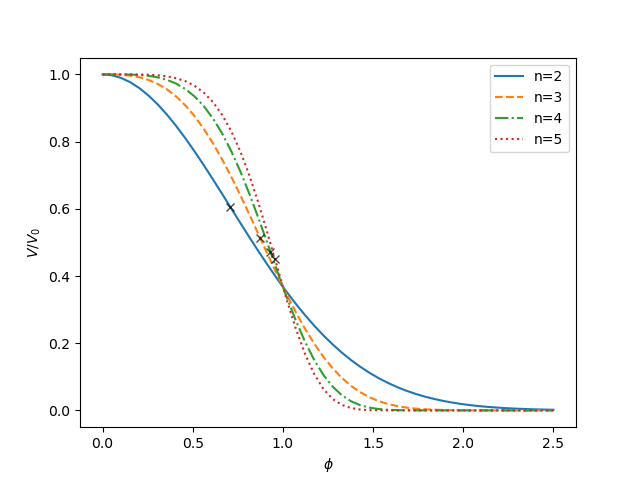
Figure 1: The form of generalized exponential potential $V(\phi)=V_{0}e^{-\alpha(\phi/M_{\rm Pl})^{n}}$, where the $\phi$ values in the x-axis are given in units of $M_{\rm Pl}$.

4 A generalized method to mould the WI power spectra in CAMB-ready forms

A good look at the WI scalar (Eq. (2.18)) and tensor (Eq. (2.23)) power spectra would tell us that these power spectra depend only on $H$, $\dot{\phi}$, $T$ and $Q$: parameters whose evolutions are determined entirely by the background dynamics of WI, given by Eq. (2.1), Eq. (2.2) and Eq. (2.3). Once we write Eq. (2.2) in terms of $T$ using Eq. (2.5), we can see that the evolution equations of $\phi$ and $T$ are coupled. For a general dissipative coefficient (Eq. (2.6)) these coupled equations can be written in terms of the $e-$foldings $N$ as

$$H(N)^{2}\phi^{\prime\prime}(N)+\left(3H(N)^{2}+\dot{H}(N)+C_{\Upsilon}M^{1-p-c}T^{p}(N)\phi^{c}(N)\right)\phi^{\prime}(N)+V,_{\phi}(\phi(N))=0,$$

$$T^{\prime}(N)+T(N)=\frac{C_{\Upsilon}M^{1-p-c}}{4C_{R}}T^{p-3}(N)\phi^{c}(N)H(N)(\phi^{\prime}(N))^{2}.$$ (4.1)

In the above set of equations $H(N)$ and $\dot{H}(N)$ can be written in terms of $\phi(N)$, $\phi^{\prime}(N)$ and $T(N)$, using the Friedmann equations given in Eqs. (2.3–2.4), as

$$H(N) = \left(\frac{V(\phi(N))+C_{R}T^{4}(N)}{3-\frac{1}{2}(\phi^{\prime}(N))^{2}}\right)^{1/2},$$ (4.2)

$$\dot{H}(N) = -\frac{1}{2}\left(H^{2}(\phi^{\prime}(N))^{2}+\frac{4}{3}C_{R}T^{4}(N)\right).$$ (4.3)

The $\phi$ equation of the coupled equations in Eq. (4.1) is a second order differential equation whereas the $T$ equation is a first order differential equation. Hence, three initial conditions, $\phi(N=0)$, $\phi^{\prime}(N=0)$ and $T(N=0)$, are required to be set for numerically evolving these equations. After the evolution one would get $\phi$, $\phi^{\prime}$ and $T$ as functions of $N$. Therefore, having $\phi(N)$, $\phi^{\prime}(N)$ and $T(N)$, all the required four quantities $\dot{\phi}(=H\phi^{\prime})$, $H$ (as given in Eq. (4.2)), $T$ and $Q(=\Upsilon/3H)$ can be obtained as functions of the $e-$folds $N$. Thus, after employing this prescription one can obtain the primordial power spectra, both the scalar and the tensor, as a function of $N$. The end of inflation is marked when $\epsilon_{H}=-\dot{H}/H^{2}=1$.

The only task remains is to relate $N$ with $k$. For that we can relate the two comoving Hubble scales, the scale when the comoving wavenumber $k_{*}$ crosses the horizon during inflation $(k_{*}=a_{*}H_{*})$, and the present Hubble scale $a_{0}H_{0}$ as [63]

$$\frac{k_{*}}{a_{0}H_{0}}=\frac{a_{*}}{a_{\rm end}}\frac{a_{\rm end}}{a_{\rm reh}}\frac{a_{\rm reh}}{a_{0}}\frac{H_{*}}{H_{0}},$$ (4.4)

where $a_{\rm end}$ and $a_{\rm reh}$ signify the scale factors at the end of inflation and the end of reheating, respectively, and we set the current scale factor $a_{0}=1$. We will show that in the cases which we will discuss, WI smoothly transits to a radiation dominated epoch, and no reheating takes place. Thus, we can set $a_{\rm end}=a_{\rm reh}$. One can relate $a_{\rm end}$ with $a_{0}$ by entropy conservation as

$$g_{s}(T_{\rm end})T_{\rm{end}}^{3}a_{\rm end}^{3}=\left(2T_{0}^{3}+\frac{21}{4}T_{\nu,0}^{3}\right)a_{0}^{3},$$ (4.5)

where $g_{s}(T_{\rm end})$ is the effective number of degrees of freedom at the end of WI, $T_{0}$ and $T_{\nu,0}=(4/11)^{1/3}T_{0}$ are the present day temperatures of the (CMB) photons and the cosmic neutrinos. Also, using $dN=d\ln a$ we see that $a_{*}/a_{\rm end}=e^{N_{*}-N_{\rm end}}$. Putting all these information together we can write Eq. (4.4) as

$$k_{*}=e^{N_{*}-N_{\rm end}}\left(\frac{43}{11g_{s}(T_{\rm end})}\right)^{1/3}\frac{T_{0}}{T_{\rm end}}H_{*}.$$ (4.6)

The values of $N_{\rm end}$ and $T_{\rm end}$ can be obtained from the evolution equation when $\epsilon_{H}=1$. We set $g_{s}(T_{\rm end})=106.75$ for definiteness, and $T_{0}=2.275$ K $=2.349\times 10^{-13}$ GeV. Using the above equation one can then numerically find the $e-$fold number $N_{P}$ when the pivot scale $k_{P}=0.05$ Mpc^-1 leaves the horizon during inflation as

$$e^{N_{P}}H_{P}=k_{P}e^{N_{\rm end}}\left(\frac{43}{11g_{s}(T_{\rm end})}\right)^{-1/3}\frac{T_{\rm end}}{T_{0}}.$$ (4.7)

Once $N_{P}$ is known, one can integrate Eq. (3.2) from $N=0$ to $N=N_{P}$ and then from $N=N_{P}$ to $N=N_{\rm end}$ to relate values of $k$ to that of $N$. Previously we have all the numerical values of the power spectra as a function of $N$, and now we have related $N$ values with $k$ values. Hence, by one-to-one mapping we now have the power spectra as functions of $k$, and these numerical values can be easily incorporated in CAMB.

This prescribed methodology has certain advantages over the ones employed before in [42, 41], such as:

• The most important advantage of this methodology is that it is applicable to any form of inflaton potential, whereas the previous methods of [42, 41] are applicable to only very simple forms of inflaton potentials, such as the quartic self-potential, and they fail when more complex inflaton potentials (such as the generalized exponential potential in Eq. (3.11)) are considered in WI.

• The methodology adopted in [42, 41] relies on slow-roll approximated dynamics of WI (for example, Eq. (3.1) and Eq. (3.6)). However, the one described here makes use of the full background dynamics of WI without any slow-roll approximation. Therefore, the power spectra (as a function of $k$) obtained using this methodology are more accurate than the ones obtained after the methods prescribed in [42, 41]. Moreover, as this methodology doesn’t require any slow-roll approximations, it can easily be generalised for WI scenarios where the dynamics depart from slow-roll, e.g. ultraslow-roll [64] or constant-roll [65].

• This methodology can be employed for any dissipative coefficient including those which cannot be written in the general form as in Eq. (2.6), e.g. the one in Eq. (2.11). The previous methods of [42, 41] are restricted only to WI models where the form of the dissipative coefficient can be written in the form as in Eq. (2.6).

5 Testing specific models of WI against the Planck data employing the prescribed generalized method

In this section, we will put to test a few WI models against the Planck data using the generalized method designed in this paper to obtain primordial power spectra as functions of $k$. First, we will discuss a model with generalized exponential potential (Eq. (3.11)) for which the previous methods described in [42, 41] fail. Then, we will verify, employing the new methodology, the results obtained in [42, 41].

5.1 WI models with generalized exponential potentials and $\Upsilon_{\rm MWI}$ as dissipative coefficient

We stated before that the generalized exponential potential of the form given in Eq. (3.11) was explored in WI in [59, 33]. In the first paper [59], the authors studied the model with $\Upsilon_{\rm cubic}$ where WI takes place in the plateau region of the potential and in weak dissipative regime. In the second paper [33], WI was studied in the steep part of the potential ($\phi>\phi_{\rm inflection}$) in the strong dissipative regime where the choice of the dissipative coefficient was $\Upsilon_{\rm MWI}$. We will examine the WI model presented in the second paper [33] with the current Planck data.

In this analysis, we will consider four different cases with $n=2,\,3,\,4,\,5$ as has been studied in [33]. We let the model parameters $g_{*}$, $V_{0}$, $C_{\Upsilon}$ and $\alpha$ float while feeding the model into Cobaya. The priors set for these model parameters are given in Table 1 which are in accordance with the choice of parameters considered in [33] (see Table 1 of [33]). To evolve the background dynamics according to Eqs. (4.1) for such models, one needs to choose the initial conditions $\phi_{0}$, $\phi^{\prime}_{0}$ and $T_{0}$, which designates the values of these parameters at $N=0$. The choice of the initial conditions as well as the best-fit model parameters are given in Table 2. One can note that the best-fit values of the model parameters obtained after the MCMC analysis through Cobaya match closely with the choice of parameters given in Table 1 of [33].

$n$	$g_{*}$		$V_{0}$ (GeV4)		$C_{\Upsilon}$		$\alpha$
	min	max	min	max	min	max	min	max
$2$	$3$	$600$	$10^{37}$	$10^{40}$	$10^{-12}$	$10^{-8}$	$7$	$15$
$3$	$3$	$600$	$10^{37}$	$10^{40}$	$10^{-12}$	$10^{-8}$	$1$	$5$
$4$	$3$	$600$	$10^{37}$	$10^{40}$	$10^{-12}$	$10^{-8}$	$0$	$3$
$5$	$3$	$600$	$10^{37}$	$10^{40}$	$10^{-12}$	$10^{-8}$	$0$	$2$

Table 1: Priors for model parameters for MCMC run.

	Initial Conditions			Model Parameters
$n$	$\phi_{0}$ (GeV)	$\phi^{\prime}_{0}$ (GeV)	$T_{0}$ (GeV)	$g_{*}$	$V_{0}$ (GeV4)	$C_{\Upsilon}$	$M$ (GeV)	$\alpha$
$2$	$5.74\times 10^{17}$	$10^{-5}$	$10^{-5}$	$124.727$	$5.63\times 10^{38}$	$5.12\times 10^{-11}$	$9.6\times 10^{5}$	$9.17$
$3$	$1.47\times 10^{18}$	$10^{-5}$	$10^{-5}$	$111.053$	$9.08\times 10^{38}$	$5.16\times 10^{-11}$	$9.6\times 10^{5}$	$3.06$
$4$	$1.91\times 10^{18}$	$10^{-5}$	$10^{-5}$	$81.7598$	$1.03\times 10^{38}$	$9.32\times 10^{-11}$	$9.6\times 10^{5}$	$1.95$
$5$	$3.27\times 10^{18}$	$10^{-5}$	$10^{-5}$	$373.185$	$7.39\times 10^{38}$	$1.75\times 10^{-10}$	$9.6\times 10^{5}$	$0.18$

Table 2: Best-fit values of the model parameters and the choice of the initial conditions.

To illustrate, we will consider the $n=2$ case. Similar results can be shown for $n=3,\,4,\,5$. The numerical values of the parameters required to determine the power spectra, $\dot{\phi}$, $H$, $T$, and $Q$, obtained after numerically evolving the coupled equations (Eqs. (4.1)) are given in Fig. 2. We also note that the model smoothly transits to a radiation dominated era after graceful exit, as shown in the left panel of Fig. 3, and we determine $N_{\rm end}-N_{P}=44.895$ using Eq. (4.7). Hence employing the method discussed in the previous section, we determine $k$ as a function of $N$ as shown in the right panel of Fig. 3.

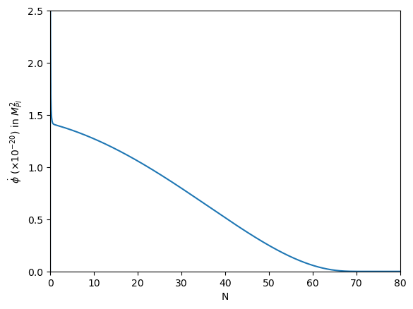
(a) Evolution of $\dot{\phi}$

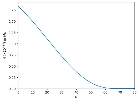
(b) Evolution of $H$

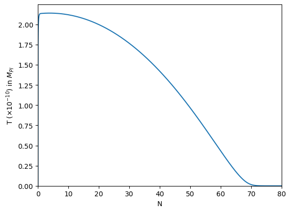
(c) Evolution of $T$

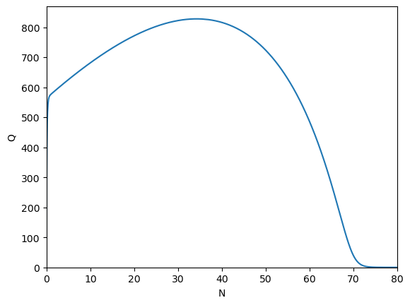
(d) Evolution of $Q$

Figure 2: Results of numerical evolution of the $n=2$ model.

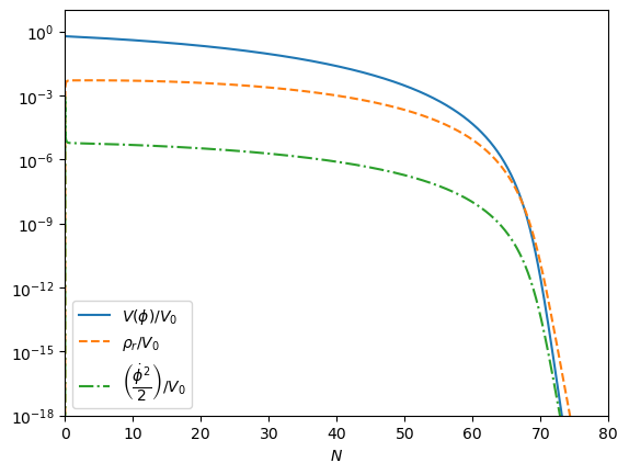
(a) Smooth transition to radiation dominated epoch after graceful exit

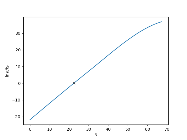
(b) $k$ vs. $N$ (the cross marks $k=k_{P}$)

Figure 3: The left panel shows that WI model with $n=2$ case smoothly transits to a radiation dominated epoch after graceful exit, whereas the right panel depicts $k$ as a function of $N$.

The scalar power spectrum in WI can be determined in two cases, one when the inflaton doesn’t thermalize with the radiation bath (thus by setting $n_{*}=0$ in Eq. (2.18)) and the other when the inflaton does thermalizes with the radiation bath (thus by setting $1+2n_{*}=\coth(H_{*}/2T_{*})$ in Eq. (2.18)). However, we note that in both these cases $1+2n_{*}$ remains subdominant by order(s) of magnitude w.r.t. the other term in the bracket in Eq. (2.18), as can be seen from Fig. 4. We plot in Fig. 5 the scalar power spectrum ${\mathcal{P}}_{\mathcal{R}}$ as a function of $k$ for both these cases to illustrate that the thermalization of the inflaton field has negligible effect of the scalar power spectrum.

Once the scalar and tensor power spectra are known as functions of $k$, one can determine the scalar spectral index $n_{s}$ and the tensor-to-scalar ratio as

$$n_{s}-1=\frac{d\ln{\mathcal{P}}_{\mathcal{R}}(k)}{d\ln(k)},\quad\quad\quad\quad r=\frac{{\mathcal{P}}_{T}}{{\mathcal{P}}_{\mathcal{R}}}.$$ (5.1)

Fig. 6 shows both $n_{s}$ and $r$ as functions of $k$ for the $n=2$ case.

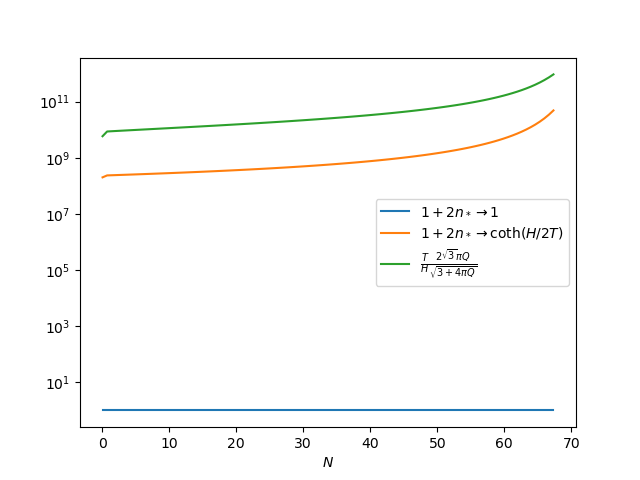
Figure 4: To illustrate that the thermalization or non-thermalization of the inflaton field during WI has insignificant effect on the scalar power spectrum of WI

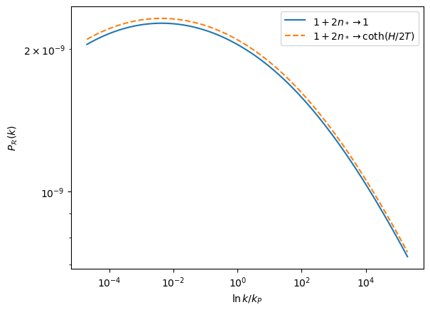
Figure 5: The scalar power spectrum as a function of $k$ for the $n=2$ case. The blue solid line (orange dashed line) depicts the power spectrum when the inflaton doesn’t (does) thermalize with the radiation bath.

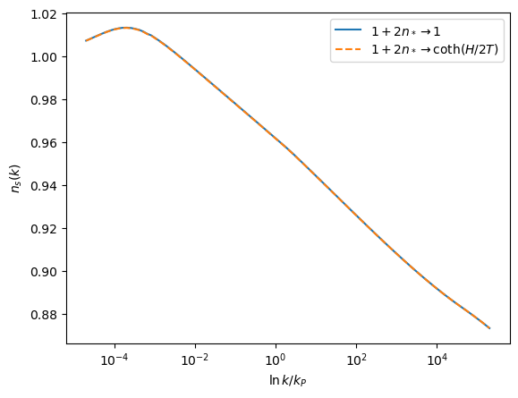
(a) $n_{s}$ as a function of $k$

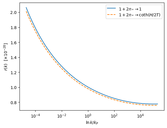
(b) $r$ as a function of $k$

Figure 6: $n_{s}$ and $r$ as a function of $k$ for the $n=2$ case. The blue solid line (orange dashed line) depicts $n_{s}$ and $r$ when the inflaton doesn’t (does) thermalize with the radiation bath.

Now coming back to all the models with $n=2,\,3,\,4,\,5$, we show the posterior distribution of all the four model parameters, $g_{*}$, $V_{0}$, $C_{\Upsilon}$ and $\alpha$ along with $\Lambda$CDM parameters, such as $\Omega_{b}h^{2}$ (baryon density parameter), $\Omega_{c}h^{2}$ (CDM density parameter), $\tau_{\rm reio}$ (reionization optical depth) and $H_{0}$ (current Hubble parameter), in Fig. 7. The posterior values of the model parameters are given in Table 3 as well. The best-fit model parameters yield the scalar amplitude $(A_{s})$, the scalar spectral index $(n_{s})$ and the running of the scalar spectral index ($\alpha_{s}=dn_{s}/d\ln k$) at pivot scale $k_{P}=0.05$ Mpc^-1 and $r$ at $k_{P}=0.002$ Mpc^-1 as given in Table 4. Note that, in [33], $r$ has been determined at $k_{P}=0.05$ Mpc^-1, and hence the values of $r$ obtained in [33] are slightly off than the ones obtained here. Moreover, values of $\alpha_{s}$ for these models have been studied in [55], and the values of $\alpha_{s}$ quoted in Table IV of [55] match reasonably well with the ones obtained here. Above all, the scalar power spectrum obtained from the best-fit model parameters fit the Planck data very well as depicted in Fig. 8. Note that all these results are quoted for $n_{*}\neq 0$ case, i.e., for the case when the inflaton thermalizes with the radiation bath.

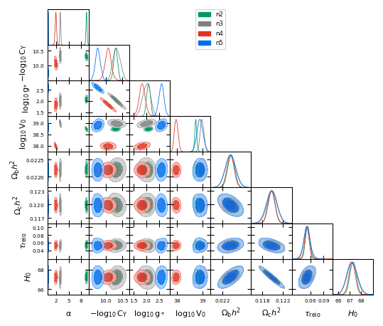
Figure 7: The posterior distribution of all the four model parameters, $g_{*}$, $V_{0}$, $C_{\Upsilon}$ and $\alpha$ along with $\Lambda$CDM parameters, such as $\Omega_{b}h^{2}$ (baryon density parameter), $\Omega_{c}h^{2}$ (CDM density parameter), $\tau_{\rm reio}$ (optical depth) and $H_{0}$ (current Hubble parameter) for cases $n=2,\,3,\,4,\,5$.

$n$	$g_{*}$	$V_{0}$ (GeV${}^{4})$	$C_{\Upsilon}$	$\alpha$
$2$	$121.62\pm 19.83$	$(5.45\pm 0.54)\times 10^{38}$	$(5.07\pm 0.65)\times 10^{-11}$	$9.22\pm 0.13$
$3$	$106.38\pm 33.91$	$(9.69\pm 1.65)\times 10^{38}$	$(4.82\pm 1.14)\times 10^{-11}$	$3.029\pm 0.098$
$4$	$70.86\pm 20.58$	$(9.53\pm 1.60)\times 10^{37}$	$(8.61\pm 1.85)\times 10^{-11}$	$1.98\pm 0.17$
$5$	$393.52\pm 87.57$	$(8.24\pm 2.25)\times 10^{38}$	$(1.74\pm 0.30)\times 10^{-10}$	$0.188\pm 0.026$

Table 3: Posterior distribution of the model parameters.

$n$	$\ln(10^{10}A_{s})$	$n_{s}$	$\alpha_{s}$	$r_{0.002}$
$2$	$3.0399$	$0.9617$	$-0.0071$	$1.15\times 10^{-28}$
$3$	$3.0407$	$0.9609$	$-0.0049$	$9.50\times 10^{-29}$
$4$	$3.0396$	$0.9638$	$-0.0043$	$1.34\times 10^{-29}$
$5$	$3.0322$	$0.9596$	$-0.0039$	$5.29\times 10^{-29}$

Table 4: $A_{s}$, $n_{s}$, $\alpha_{s}$ and $r$ from the best-fit model parameters

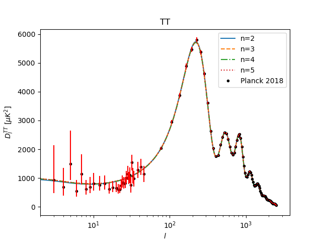
Figure 8: The CMB TT spectrum for cases $n=2,\,3,\,4,\,5$ against Planck 2018 data.

5.2 WI model with quartic potential and $\Upsilon_{\rm linear}$ as dissipative coefficient

WI model with quartic potential with $\Upsilon_{\rm linear}$ as dissipative coefficient has been studied in [42]. The analysis was done with the then current data of Planck 2015 and BICEP2/Keck Array [66, 67]. Moreover, in this paper, the number of $e-$folds is counted considering a reheating phase at the end of WI.

After evolving the background equations given in Eqs. (4.1) for this WI model, we obtained the evolution of the required parameters as functions of $N$ as shown in Fig. 9. We also see from the left panel of Fig. 10 that this model of WI, too, smoothly transits into a radiation dominated epoch. Thus, our method to determine $k$ as a function of $N$ works in this case, and we determine $N_{\rm end}-N_{P}=59.58$. The scalar power spectrum is shown in the right panel of Fig. 10 as a function of $k$. After the MCMC analysis of the model (with $n_{*}\neq 0$) against the Planck 2018 data, we show the posterior distribution of the model parameters, $g_{*}$, $\lambda$ and $C_{\Upsilon}$, and the $\Lambda$CDM parameters, $\Omega_{b}h^{2}$, $\Omega_{c}h^{2}$, $\tau_{\rm reio}$ and $H_{0}$, in Fig. 11 and Table 5. Comparing Table 5 with Table 1 of [42], one can see that both the analysis produce nearly the same best-fit model parameters. This validates the methodology prescribed in this paper.

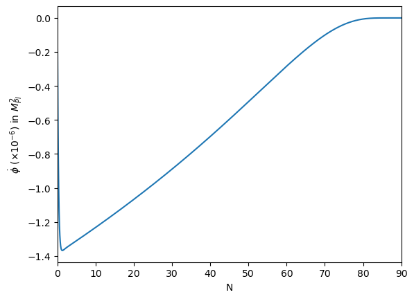
(a) Evolution of $\dot{\phi}$

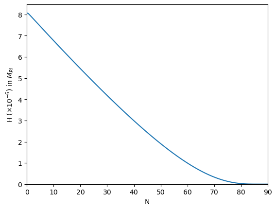
(b) Evolution of $H$

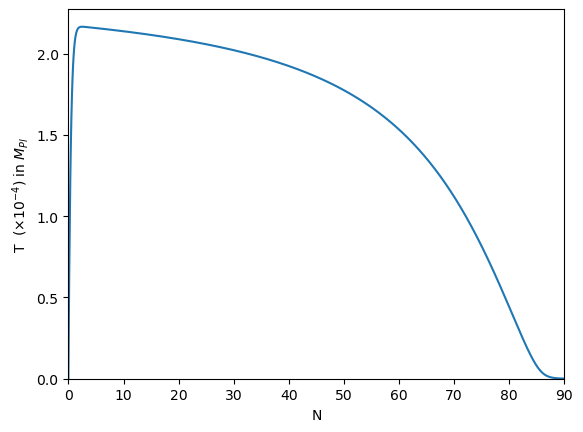
(c) Evolution of $T$

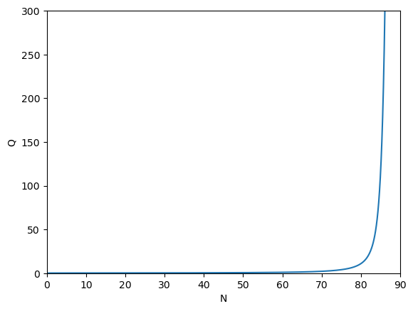
(d) Evolution of $Q$

Figure 9: Results of numerical evolution of the model studied in [42].

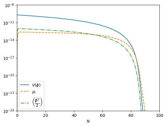
(a) Smooth transition to radiation domination

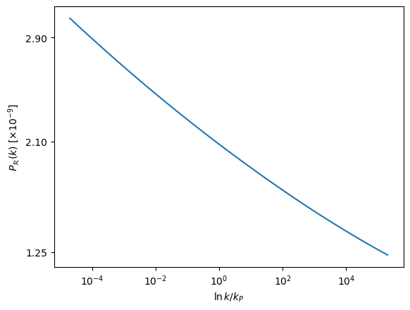
(b) Scalar power spectrum as a function of $k$

Figure 10: The left panel shows that the model studied in [42] smoothly transits into a radiation dominated epoch. The right panel plots the scalar power spectrum ${\mathcal{P}}_{\mathcal{R}}$ as a function of $k$.

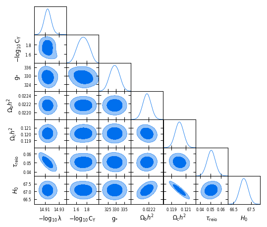
Figure 11: The posterior distribution of model parameters, $g_{*}$, $\lambda$ and $C_{\Upsilon}$ along with $\Lambda$CDM parameters, $\Omega_{b}h^{2}$, $\Omega_{c}h^{2}$, $\tau_{\rm reio}$ and $H_{0}$ for WI model studied in [42]

Parameter	$n_{*}\neq 0$
$\Omega_{b}h^{2}$	$0.02216\pm 0.00008$
$\Omega_{c}h^{2}$	$0.1201\pm 0.0006$
$-\log_{10}\lambda$	$14.914\pm 0.006$
$\lambda$	$1.219\times 10^{-15}$
$-\log_{10}C_{\Upsilon}$	$1.725\pm 0.109$
$C_{\Upsilon}$	$0.0188$
$g_{*}$	$330.917\pm 2.978$
$\tau$	$0.0502\pm 0.0041$

Table 5: Posterior distribution of the model parameters of the WI model studied in [42].

5.3 WI model with quartic potential and $\Upsilon_{\rm cubic}$ as dissipative coefficient

We will reverify the WI model having $\Upsilon_{\rm cubic}$ as dissipative coefficient with quartic potential as has been studied in [41]. In [41], the WI model has been constrained using the then available Planck 2015 data [67]. The authors keep $N_{\rm{end}}-N_{P}$ as a free parameter and chose two cases with $N_{\rm{end}}-N_{P}=50$ or 60. They also keep the value of $Q$ at the pivot scale as a free parameter.

In our prescribed methodology, $Q$ at the pivot scale is no longer a free parameter. The evolution of the required parameters as functions of $N$ are shown in Fig. 12. We note from the left panel of Fig. 13 that this WI model smoothly transits into a radiation dominated epoch post inflation, and thus one can use our methodology to relate $k$ with $N$, and we obtain $N_{\rm end}-N_{p}=61.46$ for this model. The scalar power spectrum for this model is shown as a function of $k$ in the right panel of Fig. 13. After the MCMC analysis of the model (with $n_{*}\neq 0$) against the Planck 2018 data, we show the posterior distribution of the model parameters, $g_{*}$, $\lambda$ and $C_{\Upsilon}$, along with the $\Lambda$CDM parameters, $\Omega_{b}h^{2}$, $\Omega_{c}h^{2}$, $\tau_{\rm reio}$ and $H_{0}$, in Fig. 14 and Table 6. Comparing Table 6 with Table 1 of [41] (the column for $N_{P}=60$) we note that the posterior parameters match reasonably well. This again validates the methodology prescribed in this paper.

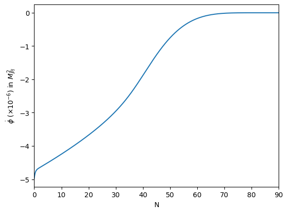
(a) Evolution of $\dot{\phi}$

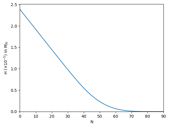
(b) Evolution of $H$

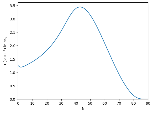
(c) Evolution of $T$

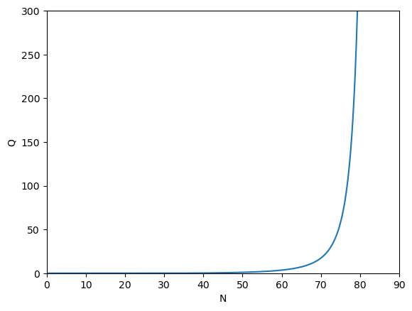
(d) Evolution of $Q$

Figure 12: Results of numerical evolution of the model studied in [41].

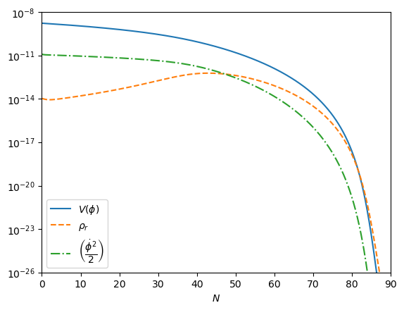
(a) Smooth transition to radiation domination

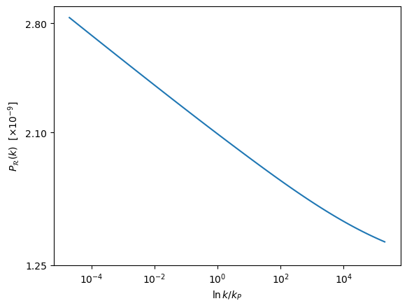
(b) Scalar power spectrum as a function of $k$

Figure 13: The left panel shows that the model studied in [41] smoothly transits into a radiation dominated epoch. The right panel plots the scalar power spectrum ${\mathcal{P}}_{\mathcal{R}}$ as a function of $k$.

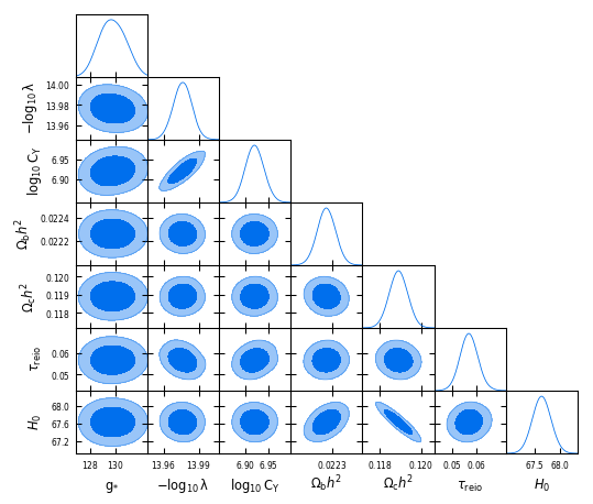
Figure 14: The posterior distribution of model parameters, $g_{*}$, $\lambda$ and $C_{\Upsilon}$ along with $\Lambda$CDM parameters, $\Omega_{b}h^{2}$, $\Omega_{c}h^{2}$, $\tau_{\rm reio}$ and $H_{0}$ for WI model studied in [41].

Parameter	$n_{*}\neq 0$
$\Omega_{b}h^{2}$	$0.02226\pm 0.00007$
$\Omega_{c}h^{2}$	$0.1189\pm 0.0004$
$-\log_{10}\lambda$	$13.976\pm 0.008$
$\lambda$	$1.057\times 10^{-14}$
$\log_{10}C_{\Upsilon}$	$6.9203\pm 0.0208$
$C_{\Upsilon}$	$8.323\times 10^{6}$
$g_{*}$	$129.638\pm 0.868$
$\tau$	$0.0569\pm 0.0038$

Table 6: Posterior distribution of the model parameters of the WI model studied in [41].

6 Conclusion

In this paper, we have devised a generalized methodology to incorporate the WI primordial power spectra, both scalar and tensor, in CAMB [8, 9] which is essential to perform a MCMC analysis of such WI models given the present cosmological data employing the publicly available codes, like CosmoMC [5, 6] or Cobaya [7]. The prescribed method is applicable to all WI models with any kind of dissipative coefficient and potential. Previous methods, as in [42, 41], were rather restrictive in the sense that they were only applicable to WI models with specific forms of dissipative coefficients, as in Eq. (2.6), and very simple forms of inflaton potentials, such as the quartic potential as has been exploited in [42, 41]. Moreover, the method prescribed in this paper employs the full background dynamics of WI, rather than the slow-roll approximated ones as required by previous methods [42, 41], and thus, is generalized enough to be extended to beyond-slow-roll dynamics of WI, such as ultraslow-roll [64] or constant-roll [65]. In addition, as the prescribed method doesn’t call for slow-roll approximated dynamics, the primordial power spectra as functions of $k$ obtained from this mechanism are more accurate than the ones one can obtain by employing previous methodologies [42, 41].

To illustrate our prescribed methodology, we analysed a WI model with generalized exponential potentials (Eq. (3.11)), a case which is not possible to analyse by the previous methodologies [42, 41] because of the complex form of such potentials. We chose $\Upsilon_{\rm MWI}$ as the dissipative coefficient and analyzed the model in the steep part of such potentials, as has been first analyzed in [33]. We did an MCMC analysis of the model parameters along with other $\Lambda$CDM parameters using the Planck 2018 data, and have shown that our analysis matches reasonably well with the parameter values chosen in [33]. We then employed our methodology to the models of those previous literature [42, 41], and showed that our results agree quite well with the results presented there. This exercise validates the functionality of our new methodology. Therefore, this new methodology that we prescribed in this paper will help put to test any model of WI against the concurrent cosmological data in future.

References

- [1] N. Aghanim et al. [Planck], Astron. Astrophys. 641, A6 (2020) [erratum: Astron. Astrophys. 652, C4 (2021)] doi:10.1051/0004-6361/201833910 [arXiv:1807.06209 [astro-ph.CO]].
- [2] P. A. R. Ade et al. [BICEP2 and Planck], Phys. Rev. Lett. 114, 101301 (2015) doi:10.1103/PhysRevLett.114.101301 [arXiv:1502.00612 [astro-ph.CO]].
- [3] Y. Akrami et al. [Planck], Astron. Astrophys. 641, A10 (2020) doi:10.1051/0004-6361/201833887 [arXiv:1807.06211 [astro-ph.CO]].
- [4] J. Martin, C. Ringeval and V. Vennin, Phys. Dark Univ. 5-6, 75-235 (2014) doi:10.1016/j.dark.2014.01.003 [arXiv:1303.3787 [astro-ph.CO]].
- [5] A. Lewis and S. Bridle, Phys. Rev. D 66, 103511 (2002) doi:10.1103/PhysRevD.66.103511 [arXiv:astro-ph/0205436 [astro-ph]].
- [6] A. Lewis, Phys. Rev. D 87, no.10, 103529 (2013) doi:10.1103/PhysRevD.87.103529 [arXiv:1304.4473 [astro-ph.CO]].
- [7] J. Torrado and A. Lewis, JCAP 05, 057 (2021) doi:10.1088/1475-7516/2021/05/057 [arXiv:2005.05290 [astro-ph.IM]].
- [8] A. Lewis, A. Challinor and A. Lasenby, Astrophys. J. 538, 473-476 (2000) doi:10.1086/309179 [arXiv:astro-ph/9911177 [astro-ph]].
- [9] C. Howlett, A. Lewis, A. Hall and A. Challinor, JCAP 04, 027 (2012) doi:10.1088/1475-7516/2012/04/027 [arXiv:1201.3654 [astro-ph.CO]].
- [10] A. Berera, Phys. Rev. Lett. 75, 3218-3221 (1995) doi:10.1103/PhysRevLett.75.3218 [arXiv:astro-ph/9509049 [astro-ph]].
- [11] V. Kamali, M. Motaharfar and R. O. Ramos, Universe 9, no.3, 124 (2023) doi:10.3390/universe9030124 [arXiv:2302.02827 [hep-ph]].
- [12] A. Berera, Universe 9, no.6, 272 (2023) doi:10.3390/universe9060272 [arXiv:2305.10879 [hep-ph]].
- [13] A. Riotto, ICTP Lect. Notes Ser. 14, 317-413 (2003) [arXiv:hep-ph/0210162 [hep-ph]].
- [14] D. Baumann, doi:10.1142/9789814327183_0010 [arXiv:0907.5424 [hep-th]].
- [15] S. S. Mishra, [arXiv:2403.10606 [gr-qc]].
- [16] R. O. Ramos and L. A. da Silva, JCAP 03, 032 (2013) doi:10.1088/1475-7516/2013/03/032 [arXiv:1302.3544 [astro-ph.CO]].
- [17] L. M. H. Hall, I. G. Moss and A. Berera, Phys. Rev. D 69, 083525 (2004) doi:10.1103/PhysRevD.69.083525 [arXiv:astro-ph/0305015 [astro-ph]].
- [18] C. Graham and I. G. Moss, JCAP 07, 013 (2009) doi:10.1088/1475-7516/2009/07/013 [arXiv:0905.3500 [astro-ph.CO]].
- [19] C. Kiefer and D. Polarski, Adv. Sci. Lett. 2, 164-173 (2009) doi:10.1166/asl.2009.1023 [arXiv:0810.0087 [astro-ph]].
- [20] C. Kiefer, I. Lohmar, D. Polarski and A. A. Starobinsky, Class. Quant. Grav. 24, 1699-1718 (2007) doi:10.1088/0264-9381/24/7/002 [arXiv:astro-ph/0610700 [astro-ph]].
- [21] C. Kiefer, D. Polarski and A. A. Starobinsky, Int. J. Mod. Phys. D 7, 455-462 (1998) doi:10.1142/S0218271898000292 [arXiv:gr-qc/9802003 [gr-qc]].
- [22] J. Martin, V. Vennin and P. Peter, Phys. Rev. D 86, 103524 (2012) doi:10.1103/PhysRevD.86.103524 [arXiv:1207.2086 [hep-th]].
- [23] S. Das, K. Lochan, S. Sahu and T. P. Singh, Phys. Rev. D 88, no.8, 085020 (2013) [erratum: Phys. Rev. D 89, no.10, 109902 (2014)] doi:10.1103/PhysRevD.88.085020 [arXiv:1304.5094 [astro-ph.CO]].
- [24] S. Das, S. Sahu, S. Banerjee and T. P. Singh, Phys. Rev. D 90, no.4, 043503 (2014) doi:10.1103/PhysRevD.90.043503 [arXiv:1404.5740 [astro-ph.CO]].
- [25] M. Bastero-Gil, A. Berera, R. O. Ramos and J. G. Rosa, Phys. Lett. B 813, 136055 (2021) doi:10.1016/j.physletb.2020.136055 [arXiv:1907.13410 [hep-ph]].
- [26] S. Bartrum, M. Bastero-Gil, A. Berera, R. Cerezo, R. O. Ramos and J. G. Rosa, Phys. Lett. B 732, 116-121 (2014) doi:10.1016/j.physletb.2014.03.029 [arXiv:1307.5868 [hep-ph]].
- [27] R. Arya, JCAP 09, 042 (2020) doi:10.1088/1475-7516/2020/09/042 [arXiv:1910.05238 [astro-ph.CO]].
- [28] M. Bastero-Gil and M. S. Díaz-Blanco, JCAP 12, no.12, 052 (2021) doi:10.1088/1475-7516/2021/12/052 [arXiv:2105.08045 [hep-ph]].
- [29] M. Correa, M. R. Gangopadhyay, N. Jaman and G. J. Mathews, Phys. Lett. B 835, 137510 (2022) doi:10.1016/j.physletb.2022.137510 [arXiv:2207.10394 [gr-qc]].
- [30] H. Motohashi and W. Hu, Phys. Rev. D 96, no.6, 063503 (2017) doi:10.1103/PhysRevD.96.063503 [arXiv:1706.06784 [astro-ph.CO]].
- [31] S. S. Mishra and V. Sahni, JCAP 04, 007 (2020) doi:10.1088/1475-7516/2020/04/007 [arXiv:1911.00057 [gr-qc]].
- [32] B. Carr, F. Kuhnel and M. Sandstad, Phys. Rev. D 94, no.8, 083504 (2016) doi:10.1103/PhysRevD.94.083504 [arXiv:1607.06077 [astro-ph.CO]].
- [33] S. Das and R. O. Ramos, Phys. Rev. D 102, no.10, 103522 (2020) doi:10.1103/PhysRevD.102.103522 [arXiv:2007.15268 [hep-th]].
- [34] S. Das, Phys. Rev. D 99, no.8, 083510 (2019) doi:10.1103/PhysRevD.99.083510 [arXiv:1809.03962 [hep-th]].
- [35] M. Motaharfar, V. Kamali and R. O. Ramos, Phys. Rev. D 99, no.6, 063513 (2019) doi:10.1103/PhysRevD.99.063513 [arXiv:1810.02816 [astro-ph.CO]].
- [36] S. Das, Phys. Rev. D 99, no.6, 063514 (2019) doi:10.1103/PhysRevD.99.063514 [arXiv:1810.05038 [hep-th]].
- [37] S. Das, Phys. Dark Univ. 27, 100432 (2020) doi:10.1016/j.dark.2019.100432 [arXiv:1910.02147 [hep-th]].
- [38] G. Obied, H. Ooguri, L. Spodyneiko and C. Vafa, [arXiv:1806.08362 [hep-th]].
- [39] S. K. Garg and C. Krishnan, JHEP 11, 075 (2019) doi:10.1007/JHEP11(2019)075 [arXiv:1807.05193 [hep-th]].
- [40] M. Benetti and R. O. Ramos, Phys. Rev. D 95, no.2, 023517 (2017) doi:10.1103/PhysRevD.95.023517 [arXiv:1610.08758 [astro-ph.CO]].
- [41] R. Arya, A. Dasgupta, G. Goswami, J. Prasad and R. Rangarajan, JCAP 02, 043 (2018) doi:10.1088/1475-7516/2018/02/043 [arXiv:1710.11109 [astro-ph.CO]].
- [42] M. Bastero-Gil, S. Bhattacharya, K. Dutta and M. R. Gangopadhyay, JCAP 02, 054 (2018) doi:10.1088/1475-7516/2018/02/054 [arXiv:1710.10008 [astro-ph.CO]].
- [43] A. Berera, I. G. Moss and R. O. Ramos, Rept. Prog. Phys. 72, 026901 (2009) doi:10.1088/0034-4885/72/2/026901 [arXiv:0808.1855 [hep-ph]].
- [44] M. Bastero-Gil, A. Berera and R. O. Ramos, JCAP 09, 033 (2011) doi:10.1088/1475-7516/2011/09/033 [arXiv:1008.1929 [hep-ph]].
- [45] M. Bastero-Gil, A. Berera, R. O. Ramos and J. G. Rosa, JCAP 01, 016 (2013) doi:10.1088/1475-7516/2013/01/016 [arXiv:1207.0445 [hep-ph]].
- [46] M. Bastero-Gil, A. Berera, R. O. Ramos and J. G. Rosa, Phys. Rev. Lett. 117, no.15, 151301 (2016) doi:10.1103/PhysRevLett.117.151301 [arXiv:1604.08838 [hep-ph]].
- [47] K. V. Berghaus, P. W. Graham and D. E. Kaplan, JCAP 03, 034 (2020) [erratum: JCAP 10, E02 (2023)] doi:10.1088/1475-7516/2020/03/034 [arXiv:1910.07525 [hep-ph]].
- [48] S. Das, G. Goswami and C. Krishnan, Phys. Rev. D 101, no.10, 103529 (2020) doi:10.1103/PhysRevD.101.103529 [arXiv:1911.00323 [hep-th]].
- [49] M. Bastero-Gil, A. Berera and R. O. Ramos, JCAP 07, 030 (2011) doi:10.1088/1475-7516/2011/07/030 [arXiv:1106.0701 [astro-ph.CO]].
- [50] M. Bastero-Gil, A. Berera, I. G. Moss and R. O. Ramos, JCAP 05, 004 (2014) doi:10.1088/1475-7516/2014/05/004 [arXiv:1401.1149 [astro-ph.CO]].
- [51] G. Montefalcone, V. Aragam, L. Visinelli and K. Freese, JCAP 01, 032 (2024) doi:10.1088/1475-7516/2024/01/032 [arXiv:2306.16190 [astro-ph.CO]].
- [52] R. M. Neal, [arXiv:math/0502099 [math.ST]].
- [53] J. Lesgourgues, [arXiv:1104.2932 [astro-ph.IM]].
- [54] S. Das and R. O. Ramos, Phys. Rev. D 103, no.12, 123520 (2021) doi:10.1103/PhysRevD.103.123520 [arXiv:2005.01122 [gr-qc]].
- [55] S. Das and R. O. Ramos, Universe 9, no.2, 76 (2023) doi:10.3390/universe9020076 [arXiv:2212.13914 [astro-ph.CO]].
- [56] C. Q. Geng, M. W. Hossain, R. Myrzakulov, M. Sami and E. N. Saridakis, Phys. Rev. D 92, no.2, 023522 (2015) doi:10.1103/PhysRevD.92.023522 [arXiv:1502.03597 [gr-qc]].
- [57] C. Q. Geng, C. C. Lee, M. Sami, E. N. Saridakis and A. A. Starobinsky, JCAP 06, 011 (2017) doi:10.1088/1475-7516/2017/06/011 [arXiv:1705.01329 [gr-qc]].
- [58] S. Ahmad, R. Myrzakulov and M. Sami, Phys. Rev. D 96, no.6, 063515 (2017) doi:10.1103/PhysRevD.96.063515 [arXiv:1705.02133 [gr-qc]].
- [59] G. B. F. Lima and R. O. Ramos, Phys. Rev. D 100, no.12, 123529 (2019) doi:10.1103/PhysRevD.100.123529 [arXiv:1910.05185 [astro-ph.CO]].
- [60] Harris, C., Millman, K., Van Der Walt, S., Gommers, R., Virtanen, P., Cournapeau, D., Wieser, E., Taylor, J., Berg, S., Smith, N. & Others Array programming with NumPy. Nature. 585, 357-362 (2020)
- [61] P. Virtanen, R. Gommers, T. E. Oliphant, M. Haberland, T. Reddy, D. Cournapeau, E. Burovski, P. Peterson, W. Weckesser and J. Bright, et al. Nature Meth. 17, 261 (2020) doi:10.1038/s41592-019-0686-2 [arXiv:1907.10121 [cs.MS]].
- [62] Hunter, J. Matplotlib: A 2D graphics environment. Computing In Science & Engineering. 9, 90-95 (2007)
- [63] A. R. Liddle and S. M. Leach, Phys. Rev. D 68, 103503 (2003) doi:10.1103/PhysRevD.68.103503 [arXiv:astro-ph/0305263 [astro-ph]].
- [64] S. Biswas, K. Bhattacharya and S. Das, Phys. Rev. D 109, no.2, 023501 (2024) doi:10.1103/PhysRevD.109.023501 [arXiv:2308.12704 [astro-ph.CO]].
- [65] S. Biswas, K. Bhattacharya and S. Das, [arXiv:2406.00340 [astro-ph.CO]].
- [66] P. A. R. Ade et al. [BICEP2 and Keck Array], Phys. Rev. Lett. 116, 031302 (2016) doi:10.1103/PhysRevLett.116.031302 [arXiv:1510.09217 [astro-ph.CO]].
- [67] P. A. R. Ade et al. [Planck], Astron. Astrophys. 594, A20 (2016) doi:10.1051/0004-6361/201525898 [arXiv:1502.02114 [astro-ph.CO]].