Theory of epigenetic switching due to stochastic histone mark loss during DNA replication

Abstract

How much information does a cell inherit from its ancestors beyond its genetic sequence? What are the epigenetic mechanisms that allow this? Despite the rise in available epigenetic data, how such information is inherited through the cell cycle is still not fully understood. Here, we develop and analyse a simple mathematical model for histone-based epigenetic information that describes how daughter cells can recapitulate the gene expression profiles of their parent. We consider the dynamics of histone modifications during the cell cycle deterministically but also incorporate the largest stochastic element: DNA replication, where histones are randomly distributed between the two daughter DNA strands. This hybrid stochastic-deterministic approach enables an analytic derivation of the switching rate, i.e., the frequency of loss-of-memory events due to replication. While retaining great simplicity, the model can recapitulate experimental switching rate data, establishing its biological importance as a framework to quantitatively study epigenetic inheritance.

1 Introduction

During the $20^{\textrm{th}}$ century, crucial breakthroughs were achieved to understand the role of nucleic acids in biological inheritance. At the beginning of the $21^{\textrm{st}}$ century, the technology to sequence and assemble the DNA of the most studied organisms was deployed. Nevertheless, our understanding of how this genetic material is regulated is still in its infancy, despite the vast amount of genetic and epigenetic data experiments can generate [17]. Reasons for our poor understanding of genetic regulation, especially in eukaryotes, include the combinatorial complexity of the interactions among genes and their products and the lack of established mechanistic and quantitative frameworks to understand vast amounts of data.

One of the most intriguing problems of gene regulation is how cells can inherit gene regulatory patterns from their ancestors. Especially in higher eukaryotes, but also in unicellular cases, different RNA expression patterns can be reliably inherited through the cellular lineage, despite all cells sharing the same underlying DNA. Often, methylation of DNA at CpG sites carries the transcriptional information required but, in many other cases, this information is carried, in the form of post-translational modifications (PTMs), by nucleosomes—histone octamers around which the DNA wraps in the eukaryotic nucleus [27, 31].

In the case of nucleosomes, since there are insufficient parental copies of them to fully occupy both daughter DNA strands after replication, they are newly synthesised by the cell in advance of S phase [6]. This implies that, after DNA replication, any histone PTMs carried within the parental cell’s DNA will be diluted in the daughter cells among the newly synthesised nucleosomes (devoid, in general, of epigenetic marks). This (on-average) two-fold serial dilution of histone marks begs the question of how such a form of memory can be stably inherited over many generations [5]. However, we know that the so-called ‘reader-writer’ enzymes are at the core of the solution to this enigma. This class of enzymatic complexes is capable of binding to particular histone PTMs (‘reading’) and spreading these same PTMs to nearby nucleosomes through their catalytic activity (‘writing’) [2]. In this way, the histone PTMs lost at replication can be recovered.

Nevertheless, loss-of-inheritance events do take place and the cause of these switching events remains uncertain. In this work, we consider a classification for the loss of inheritance in terms of the underlying cause: either replication-driven, where the perturbation due to DNA replication and the consequent dilution of histone PTMs causes the switching; or driven by the inherent stochasticity of other cellular processes (e.g., noise in read/write biochemical reactions). Leveraging this classification, we build a mathematical framework for replication-driven epigenetic switching. This framework is based on an epigenetic landscape that governs the deterministic dynamics of histone PTMs during the cell cycle, coupled to a stochastic perturbation at S phase due to DNA replication.

Previous modelling efforts have shown that the feedback mechanisms of these ‘reader-writer’ systems can yield the bistability and long-lasting memory observed in experiments [9, 4, 7, 20, 16, 13, 22]. However, these works were heavily based on numerical simulations of stochastic systems and, beyond the read-write feedback and the appearance of bistable behaviour, it has been unclear, in general, what fundamental principles govern the faithful inheritance of transcriptional information and which sources of noise could destabilise it. Here, we sought a more analytically tractable approach, which combines deterministic differential equation modelling throughout the cell cycle (which could be visualised as an epigenetic landscape) and stochastic perturbations due to DNA replication. This approach enabled us to derive simple relations for the switching rates due to replication and obtain important insights into the role of the size of these epigenetic regions.

Noteworthy in this line of research is work by Micheelsen and colleagues [15], also aimed at obtaining analytical results for this type of system. However, their approach was hindered by the complexity and stochasticity involved, which we circumvented by simplifying the problem to address replication-driven switching only. Moreover, landscape approaches have already been proposed to account for transcriptomic and epigenetic data (e.g. [28, 25, 8]), but this has usually been done in a phenomenological way, to account for heterogeneity and cell fate decisions. Here, instead, we take a bottom-up approach, placing more emphasis on the mechanisms and resolving the dynamics at the scale of the cell cycle, by taking explicitly into account the effects of replication on the epigenetic information.

This paper is structured as follows: first we motivate and introduce our epigenetic model, followed by an analytical dissection, bearing in mind the landscape analogy. Subsequently, we obtain analytical approximations for the switching rates due to replication. Finally, we compare the outputs of the model to experimental data and obtain conclusions of biological relevance.

2 Mathematical model for epigenetic switching induced by replication

Our simple, generic model for epigenetic inheritance, based on that of Ref. [9], considers acetylated $A$, unmodified $U$, and methylated $M$ nucleosomes and transitions between them: $A\leftrightharpoons U\leftrightharpoons M$ (where $A$ is associated with an active locus and $M$ with a silent one). It is a particularly well-suited model for heterochromatin in fission yeast, where these states can be related to the PTM state of histone H3 at lysine 9 (H3K9). In the spirit of replication-driven transitions, we neglect all other sources of noise in the dynamics during the cell cycle. Our approach hinges on this assumption, which allows for an extensive analysis of the system. However, there is no guarantee that in every system this will be a good approximation of the dynamics. Thus, the analysis that follows will only be valid in cases where the dilution of histone PTMs due to DNA replication is the largest source of noise.

Within this approximation, the deterministic dynamics of the concentrations of acetylated (or methylated) nucleosomes during the cell cycle in a given locus of interest, $c_{a}$ (or $c_{m}$), can be described as

$$\frac{dc_{a}}{dt} =(1-c_{a}-c_{m})(1+k_{c}c_{a})-c_{a}k_{d}(1+k_{c}c_{m})$$ (1)

$$\frac{dc_{m}}{dt} =(1-c_{a}-c_{m})(1+k_{c}c_{m})-c_{m}k_{d}(1+k_{c}c_{a}),$$ (2)

where $k_{c},k_{d}>0$, the time $t$ has been rescaled to absorb the methylation/acetylation basal rate constant, and the concentration of unmodified nucleosomes is $c_{u}=1-c_{a}-c_{m}$ due to the normalisation. For simplicity, the system has been chosen to be symmetric with respect to a $c_{a}\leftrightharpoons c_{m}$ rotation, although, in practice, it is unlikely that acetylation and methylation are exactly identical processes.

In every transition term of the model, there is a background rate and a catalytic rate (parametrised by $k_{c}$). The latter depends on the recruitment of relevant enzymes by nucleosomes present at the locus and can be related to the activity of ‘reader-writer’ enzymes, since the rate involves a product of the concentrations: its substrate (the histone they ‘write’ to) and the histone PTM to which they bind (the histone PTM they ‘read’). For appropriate parameters, these catalytic rates embody sufficiently strong feedbacks to stably maintain two fixed points, representing silenced or expressed genes. The model is schematically shown in Fig. 1B, top.

It should be noted that one of the limitations of this model is the assumption that within the genetic region of interest every nucleosome interacts with every other, allowing read-write processes between nucleosomes with equal probability regardless of how far from each other they are in physical space. While this could be a good approximation for certain small loci with a globular structure, it will become inaccurate for larger regions. Other studies have looked more precisely at this question of how the physical conformation of the chromosome affects the spreading of epigenetic marks [16, 3, 26] or sets the boundaries of regulatory regions [21, 22], but these questions lay outside of the scope of this work.

In the rest of this section we first analyse the deterministic dynamics of the model and afterwards we add the stochastic component due to replication.

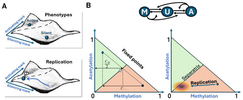
Figure 1: Landscape analogy of epigenetic regulation and inheritance. A) Illustration of the epigenetic landscape. The minima of the epigenetic landscape, whose coordinates are the abundances of specific epigenetic marks, correspond to the observable silent/active phenotypes (top). DNA replication perturbs these states by introducing unmarked nucleosomes and pushing the cell up the landscape (bottom). B) Mathematical equivalent of the landscape. The phenotypes are the fixed points of a dynamical system (left). Replication kicks the system away from the fixed point by a random distance (right), from where it will evolve in the following cell cycle. Switching occurs if the stochastic perturbation due to replication brings the system into the basin of attraction of the other fixed point, i.e., crosses the separatrix. Top: diagram of the regulatory network considered.

2.1 Fixed points

The system formed by Eqs. 1 and 2 has four fixed points, denoted by the superscript $\ast$, but only three of them in the positive $c_{a}$ and $c_{m}$ quadrant (Fig. 1B):

$$c^{*}_{a,1}= c^{*}_{m,1}=\frac{1}{k_{d}+2}$$ (3)

$$c^{*}_{a,2}= (c_{+}+c_{-})\frac{1}{2},\quad c^{*}_{m,2}=(c_{+}-c_{-})\frac{1}{2}$$ (4)

$$c^{*}_{a,3}= (c_{+}-c_{-})\frac{1}{2},\quad c^{*}_{m,3}=(c_{+}+c_{-})\frac{1}{2},$$ (5)

where

$$c_{+} =1-\frac{k_{d}}{k_{c}},$$ (6)

$$c_{-} =\frac{1}{k_{c}}\sqrt{(k_{c}-k_{d})^{2}-4}.$$ (7)

Local stability can be assessed by linear stability analysis, see Appendix A. The first fixed point is locally stable if $k_{c}<k_{d}+2$, and a saddle point otherwise. With respect to the phase space $(c_{a},c_{m})$, it is always stable in the $(1,1)$ direction, but can be unstable in the $(-1,1)$ direction. Thus, for $k_{c}>2+k_{d}$, the fixed point defined by Eq. 3 is unstable in favour of the second and third fixed points, which are now stable (see Fig. 2A for examples of trajectories in phase space).

Using a landscape as a metaphor for the dynamical system of Eqs. 1 and 2, the fixed points would be the local minima of the landscape. When evolving in time, the system would descend through the landscape, from the initial condition to the fixed point (see Fig. 1).

2.2 Separatrix

We have seen there are two stable fixed points in the dynamical system, but we would like to know, within the allowed phase space, which initial conditions would take us to one fixed point and which ones would take us to the other fixed point, i.e. the basins of attraction of each fixed point. In 2 dimensions, the separatrix is a line that separates the basins of attraction. It originates at the saddle point (if it exists) and is propagated across the phase space by the evolution of the dynamical system along the stable eigenvector of the saddle point [18].

In this case, for $k_{c}>k_{d}+2$, the separatrix passes through the point $c^{*}_{a,1}=c^{*}_{m,1}=\frac{1}{k_{d}+2}$, along the $v_{+}=(1,1)$ direction. The dynamical system along this line is symmetric, implying

$$\frac{dc_{a}}{dt}=\frac{dc_{m}}{dt}\rightarrow\frac{dc_{a}}{dc_{m}}=1.$$ (8)

Then, the separatrix is the line $c_{a}=c_{m}$, which divides the two basins of attraction of the dynamical system Eqs. 1 and 2 (Figs. 1B and 2A). In the landscape picture, the separatrix is the ridge between the valleys, separating their basins of attraction.

2.3 Replicative dilution

Given that the dynamics during the cell cycle were modelled deterministically, the only possibility for a locus in one state to switch to another one is due to a large fluctuation at replication.

The dynamical system considers the fraction of nucleosomes with a particular PTM as a continuum, which is accurate for large nucleosome numbers. In this same limit, the binomial distribution, used to model the random inheritance of nucleosomes to daughter DNA strands, can be approximated by a Normal distribution:

$$\mathcal{B}(n,p)\sim\mathcal{N}\left(np,np(1-p)\right),$$ (9)

where $n$ is the number of nucleosomes with a given PTM and $p$ is the probability of a given strand to inherit a given nucleosome.

Typically, if there is no bias in the DNA replication machinery, a standard assumption is $p=0.5$, implying that a given nucleosome can be inherited with equal probability by either DNA strand [5, 27]. Equivalently, there is a 50% probability that a given nucleosome will not be inherited onto a given daughter strand and, thus, in the daughter strand, the nucleosomal location will be occupied by a newly synthesised (unmodified) nucleosome.

In the 3-state epigenetic model we propose, $A$ or $M$ marked nucleosomes would be either inherited or replaced by unmodified nucleosomes. According to the Normal approximation, if before replication the locus had arrived at one of the steady states $(Nc_{a}^{*},Nc_{m}^{*})$ (where $N$ is the total number of nucleosomes), the probability distribution for the locus to inherit $(Nc_{a}^{i},Nc_{m}^{i})$ nucleosomes after replication is

$$P_{R}(c_{a}^{i},c_{m}^{i}|c_{a}^{*},c_{m}^{*})=\frac{2N}{\pi\sqrt{c_{a}^{*}c_{m}^{*}}}\exp\left[-2N\frac{(c_{a}^{i}-c_{a}^{*}/2)^{2}}{c_{a}^{*}}-2N\frac{(c_{m}^{i}-c_{m}^{*}/2)^{2}}{c_{m}^{*}}\right].$$ (10)

The $(c_{a}^{i},c_{m}^{i})$ pair thus constitutes the initial condition of the dynamical system for the next generation, hence determining which fixed point the locus will evolve towards. In this sense, replication can be seen as a strong perturbation that pushes the system up the landscape and if it pushes it far enough (beyond the separatrix) it will cause the switching, see Fig. 1.

We note that the assumption that the system reaches the fixed point before DNA replication is violated in certain cases [11], but we expect it to be a good approximation for many histone PTMs, especially for acetylation, which is thought to turn over on a timescale of tens of minutes [30]. However, the H3K9me3 turnover timescale is usually of the order of the cell cycle and certain other PTMs, such as those catalysed by Polycomb Repressive Complex 2, will take longer than a cell cycle to settle into a fixed point [1, 32].

A further assumption implicit in this analysis is the fact that both histone H3 copies within a given nucleosome are marked with the same PTM. While this is predominantly the case in very polarised scenarios, where most H3 histones are either acetylated or methylated, in cases where the fixed points are closer to the separatrix there could be nucleosomes with mixed PTMs, whose existence, in this model, we are neglecting.

3 Switching rate

In a system that has sufficient time to reach the fixed point during each cell cycle and whose separatrix is simply $c_{a}=c_{m}$, the switching rates are given by

$$S_{1}=\int\limits_{\begin{subarray}{c}0\leq c_{a}^{i}\leq c_{m}^{i}\leq 1\\ \textrm{s.t. }c_{a}^{i}+c_{m}^{i}\leq 1\end{subarray}}P_{R}(c_{a}^{i},c_{m}^{i}|c_{a,2}^{\ast},c_{m,2}^{\ast})dc_{a}^{i}dc_{m}^{i},$$ (11)

where $S_{1}$ is the rate of the transition from a high acetylation to a high methylation state. $S_{2}$, corresponding to the opposite transition, is equal to $S_{1}$ ($S_{2}=S_{1}=S$) given the symmetry of the model.

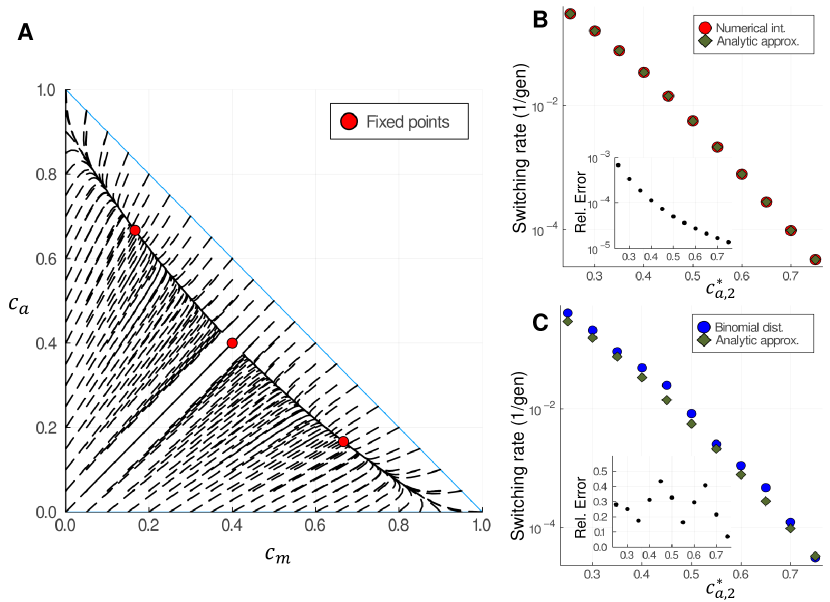
Figure 2: A) Phase diagram of the model for $k_{d}=0.5$ and $k_{c}=3$, with the dashes representing the flow on the phase portrait and the red circles, the fixed points. The separatrix is the line $c_{m}=c_{a}$, which passes through the unstable fixed point. B) Switching rates for the $c_{m}=c_{a}$ separatrix, with $c_{m,2}^{\ast}$ fixed at 0.2 and varying $c_{a,2}^{\ast}$, for both the analytic approximation Eq. 13 and the numerical integration of Eq. 11. Inset: Relative error of the analytical approximation with respect to the numerical integration. C) Same as B, but comparing the switching rates obtained from the analytical approximation Eq. 13 and the binomial distribution with $N=50$. While the relative error is of the order of 20-30%, it is still small enough not to obscure the overall trend, which spans over more than two orders of magnitude.

3.1 Analytical approximation

We can compute the integrals if we extend the integration domains:

$$S\simeq\int\limits_{-\infty<c_{a}^{i}\leq c_{m}^{i}<+\infty}P_{R}(c_{a}^{i},c_{m}^{i}|c_{a,2}^{\ast},c_{m,2}^{\ast})dc_{a}^{i}dc_{m}^{i}.$$ (12)

Note that the domains have been increased substantially (infinitely!) but most of the distribution should fall within the original integration domain, making the error of the approximation very small (see Fig. 2B, inset). Then, the integral can be evaluated analytically (see Appendix B):

$$S\simeq\frac{1}{2}\left[1-\textrm{erf}\left(\sqrt{\frac{N}{2}}\frac{c_{-}}{\sqrt{c_{+}}}\right)\right].$$ (13)

This equation for the switching rate can be interpreted as follows: $c_{-}$ is proportional to the distance of either fixed point to the separatrix (the normal distance is $c_{-}/\sqrt{2}$), explaining why the switching rate decreases with increasing $c_{-}$. In addition, a factor of $\sqrt{N/c_{+}}$ is present within the error function, which is related to the variance of the Normal distribution: the larger the number of nucleosomes the smaller the variance (in terms of fraction of the total of nucleosomes) and the smaller the switching rate.

While the approximation of Eq. 11 by Eq. 12 is very good (see Fig. 2B), approximating the binomial distribution by a Gaussian is not as accurate. To estimate the error introduced by this approximation, we rounded the continuous value of the fixed point to the nearest integer (that is $(Nc_{a}^{*},Nc_{m}^{*})\simeq(N_{a}^{*},N_{m}^{*})$, with $N_{a}^{*}$ and $N_{m}^{*}$ integers). With the integer values of the fixed points, we computed numerically the probability that replication described by a binomial distribution pushes the system out of its basin of attraction (i.e., summed the probability distribution over the other basin of attraction, including the $N_{a}=N_{m}$ case). This comparison can be seen in Fig. 2C for $N=50$, which systematically overestimates the switching rate due to the inclusion of the $N_{a}=N_{m}$ case. Nevertheless, when comparing to experimental data with $N>100$, the accuracy of the approximation increases, since the normal approximation of a binomial becomes more accurate and the finite-size effect of the separatrix (the $N_{a}=N_{m}$ case) is diluted.

Finally, it is noteworthy that these results do not depend directly on the dynamical model for the PTMs, Eqs. 1 and 2; they only depend on the fixed points and the separatrix, and the fact that we are studying replication-induced switching. More generally, if the separatrix was a line $c_{a}=\alpha\,c_{m}+\beta$ (for $\alpha>0$), the integral for the switching rates can be analogously evaluated to

$$S\simeq\frac{1}{2}\left[1-\textrm{erf}\left(\sqrt{\frac{N}{2}}\frac{c_{a,2}^{\ast}-2\beta-\alpha c_{m,2}^{\ast}}{\sqrt{c_{a,2}^{\ast}+\alpha^{2}c_{m,2}^{\ast}}}\right)\right],$$ (14)

see Appendix B for details. This last result will be useful when comparing with experimental data, see Section 4.

3.2 Assymptotic expansion

With everything else constant (in intensive parameters, which are independent of the size of the system), Eq. 13 predicts that the switching rates due to replicative dilution should decrease with increasing $N$ as

$$S\simeq\frac{1}{2}[1-\textrm{erf}(a\sqrt{N})]\sim\frac{e^{-a^{2}N}}{2a\sqrt{\pi N}},$$ (15)

where the asymptotic approximation is only valid for small switching rates and $a$ is a constant. In contrast, in Ref. [15], transitions due to noise in the biochemical reactions controlling epigenetic marks (the other source of stochasticity mentioned in the introduction) were studied and a similar exponential scaling was found: $S\propto[N\textrm{exp}(Nf)]^{-1}$, $f$ being a function related to the biochemical network.

4 Comparison with experimental data

We now seek to quantitatively compare model outputs with other relevant experimental data to emphasise the biological relevance of the model.

Loss-of-inheritance events have been quantitatively studied at a number of loci in both fission and budding yeast [23, 29]. The tractability of the yeast system has enabled significant experimental advances in the measurements of these switching events and the underlying mechanisms controlling them [24]. Thus, experimental data from the mating region in fission yeast [20] allowed us to test some of the ideas developed above.

In Ref. [20], the rates of heterochromatin establishment were measured, that is, for cells prepared in the active state, the rate at which they transitioned to the silent state. These rates were quantified for strains with DNA insertions of different lengths in the locus, effectively varying its size. From Eq. 13, the model predicts a decrease in the switching rates due to the increase in size (if all the rates, in intensive variables, remain constant). Eq. (13) has a single control parameter ($c_{-}/\sqrt{c_{+}}$) and, thus, our first attempt was to fit the heterochromatin establishment rates ($S$) as a function of nucleosome number ($N$) obtained in Ref. [20]. However, the switching rates predicted by the model decreased more slowly with $N$ than the experimental data, yielding poor quantitative agreement ($R^{2}\simeq 0.3$).

After more detailed examination, the failure of the symmetric model to reproduce the data could have been expected for a number of reasons. First, the mating region in fission yeast is typically heterochromatic, but our model is symmetric and, thus, unbiased in this sense. Second, not all reaction rates in the mating region system have intensive parameters, as our model does. In this set of experiments the genetic length of the locus was enlarged but the regulatory regions inside the locus, such as cenH, are left unchanged, and, consequently their effect is diluted within a larger locus, leading to slower heterochromatin establishment. To incorporate this, we took a phenomenological approach, by assuming that the effect of cenH and other regulatory sequences in the locus that make it heterochromatic can be captured by a shift in the separatrix, reflecting the bias towards heterochromatin (see Fig. 3A). The rationale behind this choice is that, in the absence of any PTMs (i.e. coordinate $(0,0)$ in the model), the locus should be prone to silencing solely due to the heterochromatic effect of cenH (since there cannot be any read-write feedback in the absence of histone PTMs). A shift in the separatrix would therefore capture this phenomenon.

Thus, we use Eq. 14 to explain the switching rates, with $\alpha=1$ and $\beta$ as a free parameter that represents such a shift in the separatrix. To reflect the dilution effect, the shift in the separatrix is scaled by $1/N$, effectively yielding the following expression for the switching rates:

$$S\simeq\frac{1}{2}\left(1-\textrm{erf}\left[\sqrt{\frac{N}{2}}\left(x_{1}-\frac{x_{2}}{N}\right)\right]\right),$$ (16)

where $x_{1}$ and $x_{2}$ are free parameters. The resulting least-squares fit is much more precise ($R^{2}\simeq 0.98$, see the blue line in Fig. 3B), suggesting that the dilution of the regulatory region is an important effect.

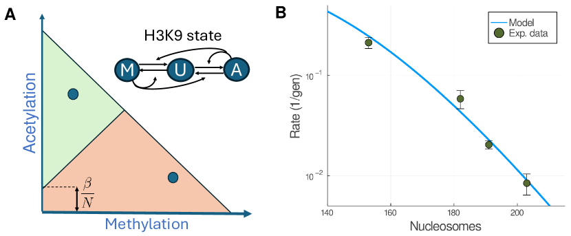
Figure 3: Comparison with experimental data. A) Phase portrait of the model for heterochromatin at the mating region in fission yeast, which is asymmetric due to the bias of the region towards the silent state. This bias is represented by the parameter $\beta$, which is divided by the number of nucleosomes $N$ to reflect the dilution effect of the regulatory region in larger loci. B) Comparison of the heterochromatin establishment rates between experiments (green data points) and the model (blue solid curve). Data and error estimation (95% confidence interval) from Ref. [20].

Consequently, our simple model can quantitatively capture experimental trends in terms of the size of the locus. This reinforces switching by replication as a key mechanism for the loss of inheritance of epigenetic information.

5 Discussion

In this paper, we have introduced a model for epigenetic memory inheritance that only considers stochastic loss-of-memory events that are due to replication. This assumption has allowed for a vast simplification of the model, which makes it analytically tractable, while maintaining a level of complexity appropriate to describe experimental data.

The model, similar to the one originally proposed in Ref. [9], is particularly well-suited for the mating region of fission yeast and, thus, we quantitatively compare it with the data available for that system. This shows an increased fidelity of the epigenetic memory (smaller switching rate) for larger loci, due to the greater number of memory units (nucleosomes). In addition, this comparison reveals the dilution effect of regulatory sequences in larger loci: by maintaining the same regulatory sequence in a larger locus, its effect decreases. Similarly, heterochromatin silencing loss in the budding yeast HMR locus was hypothesised to be replication driven and an analogous dilution effect of silencer regions was observed [14], reinforcing the generality of both the dilution effect and the replication-driven mechanism. In fact, any self-renewing cell line, not only yeast cells, must be capable of recovering their epigenetic profiles, which requires basins of attraction large enough so that the epigenetic profile can be faithfully maintained generation after generation in the face of replication-driven histone PTM dilution.

It should be noted that the experimental dataset used here was already modelled in the aforementioned paper [20], but it required much more complex models and they were exclusively based on stochastic simulations. Our approach enhances the interpretability of the model and offers closed-form relations for the switching rates, which can be checked against experimental data. From a more general perspective, this work helps establishing a classification of epigenetic switching events, dissecting them by the noise source that dominates the switching behaviour: whether it is the intrinsic noise of biochemical reactions or the dilution of epigenetic marks at replication.

However, there are also limitations in the analysis presented in this paper. The most obvious one is the generality of the network, which is only one case (a biologically motivated one) of a large number of dynamical systems that can show bistability. In particular, it is a symmetric model for the activation/silencing of loci, but acetylation and methylation might not be symmetric processes. Thus, in the future, applying an analogous analysis to other models will be instructive. In addition, we are only considering switching by replication, which is only a subset of all loss-of-memory events that could occur in cellular lineages. Finally, our knowledge of nucleosome inheritance during DNA replication is incomplete and, while the minimal hypothesis of 50% inheritance has experimental support [27], there are other experimental works suggesting lower efficiency of the nucleosome inheritance [12] or PTM-dependent inheritance [10]. Further work is needed to address the interplay between all the different sources of stochasticity, as well as alternative modes of nucleosome inheritance. Nevertheless, this work is a stepping stone towards a general and quantitative framework for epigenetics, that can help understand the regulatory logic behind the processes that maintain epigenetic memory.

Acknowledgements

We thank Govind Menon for fruitful discussions. We also thank the BBSRC Institute Strategic Programme (BB/P013511/1) and the Wellcome Human Developmental Biology Initiative for funding.

Appendix A Fixed points and stability analysis

Making use of the symmetry of the baseline, we can easily compute the fixed points, denoted by $\ast$. Adding and subtracting Eqs. 1 and 2 at steady state, with $c_{+}=c_{a}^{\ast}+c_{m}^{\ast}$ and $c_{-}=c_{a}^{\ast}-c_{m}^{\ast}$, we have

$$(1-c_{+})(2+k_{c}c_{+})-k_{d}c_{+}-2k_{d}k_{c}c_{a}^{\ast}c_{m}^{\ast}= 0$$ (17)

$$(1-c_{+})k_{c}c_{-}-k_{d}c_{-}= 0.$$ (18)

From Eq. 18, we have that either $c_{-}=0$ or $c_{+}=1-k_{d}/k_{c}$. The case $c_{-}=0$ yields the first fixed point:

$$c^{*}_{a,1}=c^{*}_{m,1}=\frac{1}{k_{d}+2}.$$ (19)

The other case, $c_{+}=1-k_{d}/k_{c}$, together with the fact $c_{a}^{\ast}c_{m}^{\ast}=(c_{+}^{2}-c_{-}^{2})/4$ and Eq. 17, yields

$$0=\frac{k_{d}}{k_{c}}(2+k_{c}-k_{d})-k_{d}\left(1-\frac{k_{d}}{k_{c}}\right)-k_{d}k_{c}\frac{\left(1-\frac{k_{d}}{k_{c}}\right)^{2}-c_{-}^{2}}{2},$$ (20)

whose solution for $c_{-}$ is

$$c_{-}=\pm\frac{1}{k_{c}}\sqrt{\left(k_{c}-k_{d}\right)^{2}-4}.$$ (21)

With a slight abuse of notation, we define $c_{-}$ as the positive solution to the previous equation and the sign is made explicit. Then, the two solutions of Eq. 21, together with $c_{+}=1-k_{d}/k_{c}$ specify the second and third fixed points of the system:

$$c^{*}_{a,2}= (c_{+}+c_{-})\frac{1}{2},\quad c^{*}_{m,2}=(c_{+}-c_{-})\frac{1}{2}$$ (22)

$$c^{*}_{a,3}= (c_{+}-c_{-})\frac{1}{2},\quad c^{*}_{m,3}=(c_{+}+c_{-})\frac{1}{2}.$$ (23)

The local stability of the fixed points can be found with a linear stability analysis. This involves obtaining the Jacobian matrix of the dynamical system, $J_{ij}=\frac{\partial f_{i}}{\partial c_{j}}|_{*}$, where $f_{i}$ are the right-hand sides of Eqs. 1 and 2 and $|_{*}$ means that they are evaluated at the fixed point of interest. The Jacobian matrix takes the form

$$J=\begin{pmatrix}-1-k_{d}-k_{c}[-1+2c_{a}+c_{m}(1+k_{d})]&-1-k_{c}c_{a}(1+k_{d})\\ -1-k_{c}c_{m}(1+k_{d})&-1-k_{d}-k_{c}[-1+2c_{m}+c_{a}(1+k_{d})]\end{pmatrix}\Bigg{|}_{\ast}$$ (24)

whose eigenvalues at the central fixed point [defined by Eq. 3] are

$$\lambda_{1}=-\frac{k_{d}(2-k_{c}+k_{d})}{2+k_{d}}$$

$$\lambda_{2}=-2-k_{c}-k_{d}.$$

The associated eigenvectors are

$$v_{1}=(-1,1)$$

$$v_{2}=(1,1),$$

implying that along the $(1,1)$ direction the fixed point is always stable, but along the $(-1,1)$ direction it is only stable if $k_{c}<2+k_{d}$ (note that all constants are greater than 0). Thus, Eq. 3 is a stable fixed point if $k_{c}<2+k_{d}$ and a saddle point otherwise.

Appendix B Switching rate integrals

The most general case of the integrals considered in Section 3 is the integral of the Normal distribution on one side of the line $y=\alpha x+\beta$. In this scenario, the switching rate integral becomes

$$S\simeq\int_{-\infty}^{+\infty}dx\int_{-\infty}^{\alpha x+\beta}dy\,\frac{2N}{\pi\sqrt{c_{a,2}^{\ast}c_{m,2}^{\ast}}}\,\textrm{exp}\left[-2N\frac{(y-c_{a,2}^{\ast}/2)^{2}}{c_{a,2}^{\ast}}-2N\frac{(x-c_{m,2}^{\ast}/2)^{2}}{c_{m,2}^{\ast}}\right].$$ (25)

For the first integral, we need the change of variable $u=\sqrt{\frac{4N}{c_{a,2}^{\ast}}}(y-c_{a,2}^{\ast}/2)$, and $du=\sqrt{\frac{4N}{c_{a,2}^{\ast}}}dy$. Then,

$$S\simeq \int_{-\infty}^{+\infty}dx\int_{-\infty}^{(\alpha x+\beta-c_{a,2}^{\ast}/2)\sqrt{\frac{4N}{c_{a,2}^{\ast}}}}du\,\frac{\sqrt{N}}{\pi\sqrt{c_{m,2}^{\ast}}}\,\textrm{exp}\left[-\frac{u^{2}}{2}-2N\frac{(x-c_{m,2}^{\ast}/2)^{2}}{c_{m,2}^{*}}\right]$$

$$= \int_{-\infty}^{+\infty}dx\,\sqrt{\frac{N}{2\pi c_{m,2}^{\ast}}}\,\textrm{exp}\left[-2N\frac{(x-c_{m,2}^{\ast}/2)^{2}}{c_{m,2}^{\ast}}\right]\left(1+\textrm{erf}\left[(\alpha x+\beta-c_{a,2}^{\ast}/2)\sqrt{\frac{2N}{c_{a,2}^{\ast}}}\right]\right).$$ (26)

From Ref. [19], we have that

$$\int_{-\infty}^{+\infty}d\tilde{x}\,\textrm{erf}(\tilde{x})e^{-(a\tilde{x}+b)^{2}}=-\frac{\sqrt{\pi}}{a}\textrm{erf}\left(\frac{b}{\sqrt{a^{2}+1}}\right).$$ (27)

In this case, $a=\frac{1}{\alpha}\sqrt{\frac{c_{a,2}^{\ast}}{c_{m,2}^{\ast}}}$ and $b=(c_{a,2}^{\ast}/2-\beta)\sqrt{\frac{2N}{c_{m,2}^{\ast}}}\frac{1}{\alpha}-\sqrt{\frac{Nc_{m,2}^{\ast}}{2}}$. Together with $\tilde{x}=(\alpha x+\beta-c_{a,2}^{\ast}/2)\sqrt{\frac{2N}{c_{a,2}^{\ast}}}$ we have

$$S\simeq \,\frac{1}{2}+\int_{-\infty}^{+\infty}d\tilde{x}\,\sqrt{\frac{c_{a,2}^{\ast}}{\pi c_{m,2}^{\ast}}}\frac{1}{2\alpha}e^{-(a\tilde{x}+b)^{2}}\textrm{erf}(\tilde{x})$$

$$= \,\frac{1}{2}-\frac{1}{2}\textrm{erf}\left(\frac{(c_{a,2}^{\ast}/2-\beta)\sqrt{\frac{2N}{c_{m,2}^{\ast}}}\frac{1}{\alpha}-\sqrt{\frac{Nc_{m,2}^{\ast}}{2}}}{\sqrt{\frac{c_{a,2}^{\ast}}{c_{m,2}^{\ast}\alpha^{2}}+1}}\right)$$

$$= \frac{1}{2}\left[1-\textrm{erf}\left(\sqrt{\frac{N}{2}}\frac{c_{a,2}^{\ast}-2\beta-\alpha c_{m,2}^{\ast}}{\sqrt{c_{a,2}^{\ast}+\alpha^{2}c_{m,2}^{\ast}}}\right)\right],$$ (28)

which corresponds to Eq. 14 in the main text.

For the symmetric baseline, where the separatrix is just $y=x$ (i.e. $\alpha=1$ and $\beta=0$), we have the result stated in the main text, Eq. 13 :

$$S\simeq\frac{1}{2}\left[1-\textrm{erf}\left(\sqrt{\frac{N}{2}}\frac{c_{a,2}^{\ast}-c_{m,2}^{\ast}}{\sqrt{c_{a,2}^{\ast}+c_{m,2}^{\ast}}}\right)\right]=\frac{1}{2}\left[1-\textrm{erf}\left(\sqrt{\frac{N}{2}}\frac{c_{-}}{\sqrt{c_{+}}}\right)\right].$$ (29)

References

- [1] C. Alabert, T. K. Barth, N. Reverón-Gómez, S. Sidoli, A. Schmidt, O. N. Jensen, A. Imhof, and A. Groth, Two distinct modes for propagation of histone ptms across the cell cycle, Genes & development, 29 (2015), pp. 585–590.
- [2] R. C. Allshire and H. D. Madhani, Ten principles of heterochromatin formation and function, Nature Reviews Molecular Cell Biology, 19 (2018), pp. 229–244.
- [3] M. Ancona, D. Michieletto, and D. Marenduzzo, Competition between local erasure and long-range spreading of a single biochemical mark leads to epigenetic bistability, Physical Review E, 101 (2020), p. 042408.
- [4] A. Angel, J. Song, C. Dean, and M. Howard, A polycomb-based switch underlying quantitative epigenetic memory, Nature, 476 (2011), pp. 105–108.
- [5] A. T. Annunziato, Split decision: What happens to nucleosomes during dna replication?*, Journal of Biological Chemistry, 280 (2005), pp. 12065–12068.
- [6] C. Armstrong and S. L. Spencer, Replication-dependent histone biosynthesis is coupled to cell-cycle commitment, Proceedings of the National Academy of Sciences, 118 (2021), p. e2100178118.
- [7] S. Berry, C. Dean, and M. Howard, Slow chromatin dynamics allow polycomb target genes to filter fluctuations in transcription factor activity, Cell systems, 4 (2017), pp. 445–457.
- [8] F. Corson and E. D. Siggia, Geometry, epistasis, and developmental patterning, Proceedings of the National Academy of Sciences, 109 (2012), pp. 5568–5575.
- [9] I. B. Dodd, M. A. Micheelsen, K. Sneppen, and G. Thon, Theoretical analysis of epigenetic cell memory by nucleosome modification, Cell, 129 (2007), pp. 813–822.
- [10] T. M. Escobar, O. Oksuz, R. Saldaña-Meyer, N. Descostes, R. Bonasio, and D. Reinberg, Active and repressed chromatin domains exhibit distinct nucleosome segregation during dna replication, Cell, 179 (2019), pp. 953–963.
- [11] D. Goodnight and J. Rine, S-phase-independent silencing establishment in saccharomyces cerevisiae, Elife, 9 (2020), p. e58910.
- [12] D. T. Gruszka, S. Xie, H. Kimura, and H. Yardimci, Single-molecule imaging reveals control of parental histone recycling by free histones during dna replication, Science advances, 6 (2020), p. eabc0330.
- [13] C. Lövkvist, P. Mikulski, S. Reeck, M. Hartley, C. Dean, and M. Howard, Hybrid protein assembly-histone modification mechanism for prc2-based epigenetic switching and memory, eLife, 10 (2021), p. e66454.
- [14] A. M. Miangolarra, D. S. Saxton, Z. Yan, J. Rine, and M. Howard, Two-way feedback between chromatin compaction and histone modification state explains Saccharomyces cerevisiae heterochromatin bistability, Proceedings of the National Academy of Sciences, 121 (2024), p. e2403316121.
- [15] M. A. Micheelsen, N. Mitarai, K. Sneppen, and I. B. Dodd, Theory for the stability and regulation of epigenetic landscapes, Physical biology, 7 (2010), p. 026010.
- [16] D. Michieletto, E. Orlandini, and D. Marenduzzo, Polymer model with epigenetic recoloring reveals a pathway for the de novo establishment and 3d organization of chromatin domains, Physical Review X, 6 (2016), p. 041047.
- [17] J. E. Moore, M. J. Purcaro, H. E. Pratt, C. B. Epstein, N. Shoresh, J. Adrian, T. Kawli, C. A. Davis, A. Dobin, et al., Expanded encyclopaedias of dna elements in the human and mouse genomes, Nature, 583 (2020), pp. 699–710.
- [18] J. D. Murray, Mathematical Biology: I. An Introduction, vol. 17, Springer Science & Business Media, 2007.
- [19] E. W. Ng and M. Geller, A table of integrals of the error functions, Journal of Research of the National Bureau of Standards B, 73 (1969), pp. 1–20.
- [20] J. F. Nickels, A. K. Edwards, S. J. Charlton, A. M. Mortensen, S. C. L. Hougaard, A. Trusina, K. Sneppen, and G. Thon, Establishment of heterochromatin in domain-size-dependent bursts, Proceedings of the National Academy of Sciences, 118 (2021), p. e2022887118.
- [21] J. F. Nickels and K. Sneppen, Confinement mechanisms for epigenetic modifications of nucleosomes, PRX Life, 1 (2023), p. 013013.
- [22] J. A. Owen, D. Osmanović, and L. Mirny, Design principles of 3d epigenetic memory systems, Science, 382 (2023), p. eadg3053.
- [23] L. Pillus and J. Rine, Epigenetic inheritance of transcriptional states in s. cerevisiae, Cell, 59 (1989), pp. 637–647.
- [24] L. N. Rusche, A. L. Kirchmaier, and J. Rine, The establishment, inheritance, and function of silenced chromatin in saccharomyces cerevisiae, Annual review of biochemistry, 72 (2003), pp. 481–516.
- [25] M. Sáez, J. Briscoe, and D. A. Rand, Dynamical landscapes of cell fate decisions, Interface focus, 12 (2022), p. 20220002.
- [26] S. H. Sandholtz, Q. MacPherson, and A. J. Spakowitz, Physical modeling of the heritability and maintenance of epigenetic modifications, Proceedings of the National Academy of Sciences, 117 (2020), pp. 20423–20429.
- [27] G. Schlissel and J. Rine, The nucleosome core particle remembers its position through dna replication and rna transcription, Proceedings of the National Academy of Sciences, 116 (2019), pp. 20605–20611.
- [28] A. E. Teschendorff and A. P. Feinberg, Statistical mechanics meets single-cell biology, Nature Reviews Genetics, 22 (2021), pp. 459–476.
- [29] G. Thon and T. Friis, Epigenetic inheritance of transcriptional silencing and switching competence in fission yeast, Genetics, 145 (1997), pp. 685–696.
- [30] J. H. Waterborg, Dynamics of histone acetylation in saccharomyces cerevisiae, Biochemistry, 40 (2001), pp. 2599–2605.
- [31] A. Wenger, A. Biran, N. Alcaraz, A. Redó-Riveiro, A. C. Sell, R. Krautz, V. Flury, N. Reverón-Gómez, V. Solis-Mezarino, M. Völker-Albert, et al., Symmetric inheritance of parental histones governs epigenome maintenance and embryonic stem cell identity, Nature Genetics, 55 (2023), pp. 1567–1578.
- [32] B. M. Zee, R. S. Levin, B. Xu, G. LeRoy, N. S. Wingreen, and B. A. Garcia, In vivo residue-specific histone methylation dynamics, Journal of Biological Chemistry, 285 (2010), pp. 3341–3350.