Minimum-regret hydrogen supply chain strategies to foster the energy transition of European hard-to-abate industries
Abstract
Low-carbon hydrogen (\ceH2) is envisioned to play a central role in decarbonizing European hard-to-abate industries, such as refineries, ammonia, methanol, steel, and cement. To enable its widespread use and support the transition, low-carbon \ceH2 supply chain (HSC) infrastructure is required. Mature and economically viable low-carbon \ceH2 production pathways include steam methane reforming of natural gas coupled with carbon dioxide (\ceCO2) capture and storage, water-electrolysis from renewable electricity, biomethane reforming, and biomass gasification. However, uncertainties surrounding demand and feedstock availabilities hamper their proliferation. Therefore, this work investigates the impact of uncertainty in future \ceH2 demands and biomass availability on the HSC design. The HSC is modeled as a network of \ceH2 production and consumption sites that are interconnected by \ceH2 and biomass transport technologies. \ceCO2 capture, transport, and storage infrastructure is modeled alongside the HSCs. We determine the cost-optimal low-carbon HSC design by solving a linear optimization model, considering a regional spatial resolution and a multi-year time horizon from 2022 to 2050. We adopt a scenario-based uncertainty quantification approach and define discrete scenarios with varying \ceH2 demands and biomass availability. Applying a minimum-regret strategy, we show that planning for sufficiently large low-carbon \ceH2 production capacities (about 9.6 Mt/a by 2030) is essential to flexibly scale up HSCs and accommodate larger \ceH2 demands of up to 35 Mt/a by 2050. Although biomass-based hydrogen production technologies are identified as the most cost-efficient low-carbon hydrogen production technologies, investments are not recommended unless the availability of biomass feedstocks is guaranteed. In this context, investments in SMR-CCS and electrolyzers often offer greater flexibility. Furthermore, we highlight the importance of \ceCO2 capture, transport, and storage infrastructure in the transition, which is required across scenarios. In particular the availability of \ceCO2 removal technologies determine the ability to realize the 2050 net-zero emissions target.
keywords:
hydrogen economy , uncertainty quantification , hard-to-abate industries , min-regret strategy , hydrogen supply chains , carbon dioxide capture, transport and storage infrastructure ,[a]organization=Institute of Energy and Process Engineering,city=Zürich, postcode=8092, country=Switzerland
[b]organization=RWTH Aachen University,city=Aachen, postcode=52062, state=North Rhine-Westphalia, country=Germany
1 Introduction
The envisioned role of hydrogen (\ceH2) in the future energy system has changed significantly throughout the years [1, 2]. Nevertheless, interest in \ceH2 remains high, and its potential to decarbonize industrial sectors is widely acknowledged [3, 4]. The European industrial sector is currently responsible for 752 Mt (21 %) of the annual anthropogenic greenhouse gas (GHG) emissions [5]. Major contributors are the cement industry (15 %), the iron and steel industry (14 %), and the chemical industry, which includes refineries, methanol, and ammonia production (18 %) [6]. These industries are difficult to decarbonize as they inherently rely on carbonaceous feedstocks and high-temperature heat, and therefore, are often referred to as "hard-to-abate" industries.
Efficiency improvements can reduce process emissions to an extent [7, 8], however, additional measures are required to achieve the impending emissions targets, such as the EU Fit for 55 target, which requires a 55 % emission reduction with respect to 1990, and the net-zero \ceCO2 emissions target for 2050 [9]. Hence, a shift to low-carbon feedstocks and energy carriers is required. In this context, \ceH2, produced with low \ceCO2 emissions (i.e., low-carbon \ceH2) is viewed as a promising solution. In Europe, \ceH2 qualifies as "low-carbon" if process emissions are below 4.42 kgCO2/kgH2 [10].
About 9 % (8.2 Mt) of the global \ceH2 demand is currently (2022) produced and consumed in Europe [11], 85 % of which is used as a feedstock to produce ammonia, methanol and other chemicals, or in refineries [12]. Aside from the current use of \ceH2 as a feedstock, low-carbon \ceH2 has the potential to replace coal as a reducing agent in the steel-making process [13], to generate high-temperature heat required in the cement-making process [14], or, combined with captured \ceCO2, to replace carbonaceous feedstocks in chemicals production (e.g., methanol and plastics) [15].
However, the future demand for low-carbon \ceH2 is deeply uncertain. Governmental institutions (e.g., [16, 17, 18]) and energy consultancies (e.g., [3, 13, 19]) investigate the potential of low-carbon \ceH2 for decarbonizing European hard-to-abate industries and provide demand estimates for 2030 and 2050. Their 2050 demand estimates range from 2.4 Mt to 40 Mt. To enable the widespread use of low-carbon \ceH2, a European supply chain (HSC) infrastructure is required [20, 21]. However, the infrastructure development is strongly dependenant on the projections and assumptions surrounding future low-carbon \ceH2 demands [22, 23].
In general, low-carbon \ceH2 can be produced starting from renewable electricity via water-electrolysis and from biomass via biomass gasification or biomethane reforming [24]. Furthermore, \ceH2 production from natural gas via steam methane reforming coupled with \ceCO2 capture and storage (CCS) can be considered low-carbon if \ceCO2 capture rates exceed 90 % and leakage rates of natural gas supply chains below 0.2 % [25]. A comparison of the available low-carbon \ceH2 production routes identifies biomass-based \ceH2 production as the most cost-efficient alternative while offering large reductions in \ceCO2 emissions; especially when coupled with CCS, it enables net-negative emissions [26]. However, difficulties in biomass collection, a lack of infrastructure, and competing interests with other sectors may substantially reduce the amount of biomass that can be dedicated for low-carbon \ceH2 production [27, 28, 29]. Therefore, the uncertainty in biomass availability must be considered when planning low-carbon HSCs.
Energy system optimization models have proven to provide useful insights for energy planners and policymakers [30]. They are widely used to investigate HSCs, offering an integrated representation of \ceH2 production and transport, and enabling the analysis of trade-offs between technology alternatives over long-term, multi-period time horizons [31]. However, a key challenge lies in the uncertainty associated with the input data of energy system optimization models [32], and accuracy assessments reveal that energy system optimization models systematically underestimate uncertainties [33, 34, 35]. Therefore, the uncertainty should be accounted for in the decision-making process to increase robustness and derive long-term policy recommendations [36, 32].
[37] perform an extensive literature review of existing HSC models. While most HSC models are deterministic, several works exist that include uncertainty, with [38, 39] leading the way. Thus far, many studies pertain to the uncertainty in the \ceH2 demand, e.g. [40, 23, 41, 42], which is identified as the most influential parameter for the HSC design [22].
Four approaches are commonly used to address the uncertainty in the input data: (1) Monte Carlo analysis (e.g., [41]), (2) stochastic programming (e.g., [39, 43]), (3) robust optimization (e.g., [44]), and (4) scenario-based uncertainty analysis (e.g., [45]). While (1)-(3) provide clear recommendations to decision-makers by directly accounting for the uncertainty in the input data, they also largely increase the model complexity making it difficult to maintain feasibility. Considering computational limitations, scenario-based approaches are often better suited to include uncertainty in large-scale energy system models [32]. Min-max regret criteria can be used to hedge against parameter variations and identify the solution that performs best, even in the worst case [46].
To the best of our knowledge, no uncertainty analysis of the European HSC infrastructure rollout exists to date. This work aims to address this gap and identifies minimum-regret strategies that result in the lowest costs considering the deep uncertainty surrounding the future \ceH2 demand and the availability of biomass feedstocks for \ceH2 production. In particular, we investigate (1) how uncertainties in the future \ceH2 demand and biomass feedstock availability influence the optimal design and rollout of HSC and \ceCO2 infrastructures, and (2) what \ceH2 production technologies, feedstocks, and energy sources are consistently deployed in the optimum HSC infrastructure design of the future.
The paper is structured as follows. Section 2 describes the considered system (Section 2.1), the uncertainty quantification approach for \ceH2 demand and biomass availability (Section 2.2 and Section 2.3, respectively), and the solution strategy used to investigate the optimal HSC under uncertainty and identify the minimum-regret strategy (Section 2.4 and Section 2.5, respectively). Section 3 presents the results and Section 4 discusses their implications. Finally, Section 5 draws conclusions.
2 Optimal design of hydrogen supply chains (HSCs) under uncertainty
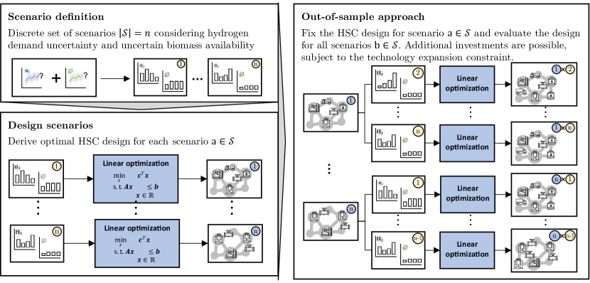
The elements of the analyzed HSCs are described in Section 2.1. Furthermore, Fig. 1 visualizes the methodology developed to identify the minimum-regret HSC design considering uncertainties in future \ceH2 demands and biomass availability. "Scenario definition" derives a discrete set of scenarios by combining the \ceH2 demand and biomass availability projections (Sections 2.2 and 2.3). "Design scenario" determines the optimal HSC design for each scenario using a deterministic, linear optimization model outlined in Section 2.4. The resulting HSC design describes the optimal low-carbon \ceH2, \ceCO2, and biomass infrastructure rollout for a given \ceH2 demand and biomass availability; allowing governments to deduce policies promoting low-carbon technologies and incentivizing manufacturers to ramp up their capacities to enable the rapid scale-up of low-carbon technology capacities and infrastructure. "Out-of-sample approach" evaluates the HSC designs derived in "Design scenario", when operated under all other possible scenarios . Additional investments may be needed to adapt the initial supply chain design derived under scenario to meet the target decarbonization pathway under the new conditions of scenario . However, these additional investments, and thus, the speed at which technology capacities can be expanded, are limited by the existing and planned capacities of the technology manufacturers [47]. We include this by adding a technology expansion constraint to the optimization model, which estimates the speed of the technology expansion based on the existing capacity stocks (Section 2.4 and Section S3). Finally, the performance of each design scenario of the HSC is evaluated based on the levelized cost of \ceH2 (LCOH) of the out-of-samples scenarios. The minimum-regret solution is the design scenario, for which (i) the highest cost of the out-of-sample scenario is the lowest across all design scenarios (i.e. the min-max LCOH) and (ii) all out-of-sample scenarios meet the annual emission targets (Section 2.5).
2.1 System description
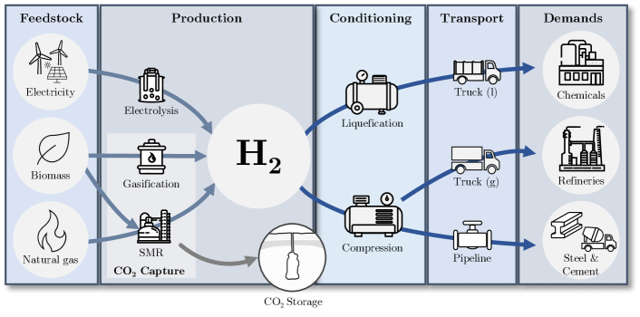
The HSC is modeled as a network of nodes and edges, with regional resolution following the EU’s Nomenclature of territorial units for statistics for level 2 (NUTS 2) [48]. At each node, \ceH2 can be produced through a portfolio of feedstocks and energy sources, including natural gas, electricity, and biomass. To reduce \ceCO2 emissions, \ceH2 production from natural gas and biomass can be coupled with \ceCO2 capture technologies. Edges connect the nodes. The distance between two nodes is approximated by their Haversine distance. At each edge, \ceH2, \ceCO2, and biomass transport technologies can be installed. In the following, the individual components of the supply chain are described in more detail. Fig. 2 provides an overview of the available feedstocks and energy sources, the available \ceH2 production and transport technologies, and the considered \ceH2 demands. The full model description is published in [49].
Feedstocks and energy sources.
The considered feedstocks and energy sources are natural gas, electricity, and biomass. We assume that natural gas and grid electricity are available at each node. Furthermore, renewable electricity can be generated from wind and solar energy. The wind and solar energy potentials are modeled as the technical potentials reported in [50, 51]. Furthermore, the availability of biomass is subject to uncertainty and limited according to the selected scenario (Section 2.3).
\ceH2 production technologies
The available \ceH2 production technologies are (i) steam methane reforming (SMR) from natural gas or biomethane, (ii) water-electrolysis from electricity, and (iii) biomass gasification. SMR and biomass gasification can be coupled with \ceCO2 capture and storage to lower process emissions. The techno-economic parameters of the \ceH2 production technologies are reported in Section Section S1.2.
\ceH2 transport technologies
The available \ceH2 transport technologies are trucks and pipelines. The transport conditions for \ceH2 vary depending on the transport mode. Trucks transport \ceH2 in ISO-tank containers (isotainers) as a compressed gas or in its liquid form (\ceH2 truck gas and \ceH2 truck liquid), and pipelines transport \ceH2 as a compressed gas. To meet the specific transport requirements, \ceH2 is conditioned (i.e., compressed or liquefied). The techno-economic parameters of the \ceH2 transport and conditioning technologies are reported in Section Section S1.2.
\ceH2 demand
Current (2020) and potential future \ceH2 demands for ammonia production, methanol production, refineries, steel production, and cement production are considered. To account for the uncertainty in future \ceH2 demands, different \ceH2 demand scenarios are investigated (Section 2.2 and Section S2).
\ceCO2 supply chain
A \ceCO2 supply chain is designed alongside the \ceH2 supply chain to account for the transport of the \ceCO2 captured at the production sites to the storage locations. We consider 27 potential \ceCO2 storage locations in Europe following [52]. The \ceCO2 storage capacity is limited by the capacity of existing and announced \ceCO2 storage projects, which corresponds to 132 Mt/a [52]. The available \ceCO2 transport technologies are trucks (with isotainers) and pipelines. Similarly to \ceH2, the captured \ceCO2 is conditioned to meet transport requirements. The techno-economic parameters for \ceCO2 transport are reported in Section Section S1.2.
Biomass supply chain
Two types of biomass are considered: dry and wet biomass. Dry biomass consists of woody biomass, which can be transported for long distances via containers loaded on trucks [53, 28]. Wet biomass consists of manure and waste biomass, whose collection and transport is challenging [28], with maximum transport distances ranging between [28, 54]. Therefore, we assume that wet biomass cannot be transported and is only used at the locations where it is available. Wet biomass serves as feedstock for anaerobic digestion to produce biomethane, which can be transported via isotainers loaded on trucks [55] or injected into the natural gas grid [13]. We assume that the gas grid is available at each node of the supply chain, and that biomethane can be injected into the gas grid subject to grid connection costs [13]. The techno-economic parameters for dry biomass transport and biomethane transport are reported in Section Section S1.2.
2.2 Hydrogen demand uncertainty
The uncertainty analysis covers \ceH2 demand predictions for European hard-to-abate industries, namely refineries, ammonia, methanol, steel, and cement industries. A literature search is conducted to collect \ceH2 demand forecasts for the different industries and covers publications from 2018 to today. In total, 28 literature scenarios are analyzed (Table 1). Scenarios that do not provide a breakdown of the \ceH2 demand estimates for the considered industries are excluded from further analysis.
The feasibility and attractiveness of hydrogen-based solutions is influenced by technological, economic, and political factors. Uncertainties surrounding technological factors such as technological breakthroughs and the time required for commercialization, as well as uncertainty surrounding economic factors such as the cost-competitiveness of low-carbon \ceH2 technologies and the uncertainty surrounding future cost trajectories can hinder their adoption. In contrast, political measures such as \ceCO2 pricing mechanisms can address affordability issues and promote investments [31, 56].
In particular, assumptions surrounding (1) material and process efficiency, (2) electrification, (3) recycling, and (4) \ceCO2 capture and storage strongly influence the \ceH2 demand predictions [57]. For example, in ammonia production, material and process efficiency improvements could reduce \ceH2 feedstock requirements by up to 25 % with respect to today’s values [57]. In steel industry, recycled (or secondary) steel could replace 50-70 % of the primary steel production, thereby reducing potential future \ceH2 demands substantially [58]. The availability of electricity-based decarbonization pathways and the option of \ceCO2 capture and storage add further layers of uncertainty [59].
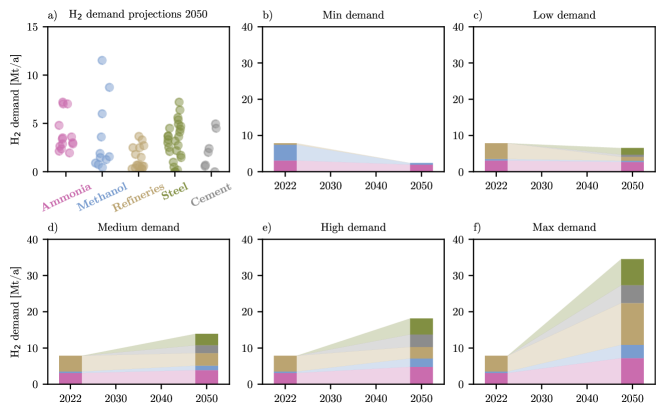
Fig. 3a visualizes the 2050 \ceH2 demand estimates for the considered industries reported across literature (Table 1). In general, the spread of projected \ceH2 demands is lower in industries that inherently rely on \ceH2 as a feedstock in their production process (ammonia production plants and refineries). The spread increases for industries where multiple decarbonization strategies compete with each other (e.g., steel and cement industry). The largest spread is observed for methanol, an important base chemical that is required e.g., for plastics production via the methanol-to-olefins route. While [13, 14] expect a large uptake of methanol-to-olefins, and thus, the methanol demand, [3] provide more conservative methanol demand estimates. Section S2 provides a detailed analysis of the variability in the regional \ceH2 demand estimates.
| Title | No. Scenarios | 2050 demand [Mt/a] | Industries | Source |
|---|---|---|---|---|
| 12 insights on hydrogen | 2 | 6.6-14.5 | Chemicals, Steel, Refineries | [60] |
| No-regret hydrogen | 1 | 8.1 | Chemicals, Steel, Refineries | [3] |
| Navigating through hydrogen | 3 | 8.0-18.6 | Chemicals, Steel, Refineries | [19] |
| Clean planet for all | 11 | 0-18.5 | Chemicals, Steel, Refineries, Cement | [17] |
| Hydrogen roadmap | 2 | 2.5-5.6 | Steel | [61] |
| The optimal role for gas in a net zero emissions energy system | 1 | 9.9 | Chemicals, Steel, Refineries, Cement | [13] |
| Analysing future demand, supply, and transport of hydrogen | 1 | 733 | Chemicals, Steel, Refineries, Cement | [14] |
| The potential of hydrogen for decarbonising EU industry | 2 | 6.3-18.8 | Chemicals, Refineries, Steel | [62] |
| Hydrogen roadmap europe | 2 | 12.2-19.6 | Chemicals, Steel, Refineries, Cement | [63] |
| Industrial transformation 2050 | 3 | 5.6-10.7 | Chemicals, Steel, Cement | [57] |
Five \ceH2 demand scenarios are developed to tackle the deep uncertainty associated with the future \ceH2 demands: minimum (min), low, medium, high, and maximum (max). The medium demand scenario represents the average of the \ceH2 demand estimates. The low and high demand scenarios are derived based on the 25th and 75th quartile of the \ceH2 demand estimates. Quartiles are used here because they are insensitive to outliers, but maintain the information about the center and spread of the \ceH2 demand estimates [64]. Finally, the min and max demand scenarios represent the minimum and maximum \ceH2 demand estimates, and are added to cover the full range of the \ceH2 demand estimates. Fig. 3b-f visualize the temporal evolution of the five \ceH2 demand scenarios, where data is collected for 2020 and 2050, and linear interpolation is used for intermediate years.
2.3 Biomass availability uncertainty
[53] and [65] estimate the technical and sustainable potential, respectively, of bioenergy for different types of biomass in Europe. However, the availability of biomass feedstocks is highly uncertain, and sustainability and socio-political factors such as the competition of biomass feedstocks with food production or alternative land uses are often not accounted for [66]. Here, we focus on sustainable biomass potentials, i.e. biomass that is not primarily grown for energy use and does not compete with food production or alternative land uses. Sustainable biomass includes residues from agriculture and forests and animal manure [67].
To account for the uncertainty in biomass availability, we define three discrete scenarios: a reference scenario, a scenario with reduced biomass availability to account for competition with other sectors, and a scenario where no biomass is available for low-carbon \ceH2 production. In the reference scenario, the estimates from [65] are used. In the scenario with reduced biomass availability, we assume that the sectoral biomass consumption is proportional to the sectoral primary energy demands. According to the EU reference scenario, 26 % of the total energy consumption can be attributed to industry. Thus, in the reduced biomass scenario, only 26 % of the sustainable biomass potential is available for low-carbon \ceH2 production.
2.4 Optimization model
The optimal design of the HSC is determined via a linear optimization problem following [49]. In general form, a linear optimization problem can be formulated as follows:
| (1) |
where the objective function is expressed as a linear combination of continuous decision variables with dimension and coefficients ; and the constraints are expressed as a linear combination of matrix , decision variables , and vector .
The optimization problem is implemented in the optimization framework ZEN-garden (Zero-emissions Energy Networks), developed at the Reliability and Risk Engineering Lab at ETH Zurich. ZEN-garden optimizes the design and operation of energy system models to investigate transition pathways toward decarbonization [49, 68, 69]. The optimization problem is solved using the commercial solver Gurobi [70].
Input Data
The input data to the optimization problem includes (i) spatially-resolved \ceH2 demands, carrier prices, \ceCO2 intensities, and availabilities of biomass, wind, and solar energy, (ii) the techno-economic parameters describing the cost and performance of production, conditioning, and transport technologies, (iii) the existing \ceH2 production capacities, (iv) the size and location of the available \ceCO2 storage sites, and (v) the target decarbonization pathway. A yearly resolution is used to model the time-dependent variables, namely the \ceH2 demands, carrier prices, \ceCO2 intensity of the electricity grid, and biomass availability. The input data is reported in Section S1.
Decision Variables
The optimization problem determines (i) the optimal selection, capacity, and location of the \ceH2 production, conditioning, and transport technologies, (ii) the energy inputs and outputs of each \ceH2 production and conditioning technology, (iii) the carrier flows through each transport technology, (iv) the nodal carrier imports and exports.
Constraints
The constraints of the optimization problem include (i) the nodal mass balances for electricity, natural gas, \ceH2, biomass, and \ceCO2, (ii) the performance and operating limits of the \ceH2 production, conditioning, and transport technologies, and (iii) the \ceCO2 emissions constraint limiting the yearly \ceCO2 emissions to the target emissions values of the selected decarbonization pathway. Here, we assume linearly decreasing \ceCO2 emissions from today’s values such that the 2050 net-zero emissions (NZE) target is achieved [71]. To ensure the feasibility of the optimization problem, a slack variable is added to the \ceCO2 emission constraint. This slack variable can be interpreted as a \ceCO2 emissions overshoot of the emission target and is associated with a large cost (100k€/ t), ensuring that overshooting the \ceCO2 emission constraint is selected as a last resort. The HSC design is considered a feasible solution if the \ceCO2 emissions target is achieved and the \ceCO2 emissions overshoot is zero.
The constraints are detailed in [49]. Here, we expand the model formulation from [49] by adding technology expansion constraints when performing the out-of-sample approach (Fig. 1). The technology expansion constraints limit the maximum annual growth rate of a technology based on the existing capacity stock and are formulated following [47, 69] and described in Section S3. The technology expansion is parameterized based on historically observed growth rates. [69] investigate the historical annual growth rates for low-carbon technologies and observe growth rates between 10 % (wind offshore) to 29 % (solar PV). For our reference case, we select a technology expansion rate of 20 %. A sensitivity analysis is performed for technology expansion rates varying from 10 % to 29 %.
Objective function
The optimization problem minimizes the net present cost of the system, which includes the investment and operating costs of the \ceH2, \ceCO2, and biomass supply chains in compliance with the \ceCO2 emission targets.
2.5 Minimum-regret solution
The minimum regret solution is the HSC scenario design that (i) results in the lowest levelized cost of \ceH2 (LCOH) for the worst-case out-of-sample scenario (i.e., the min-max across the LCOH of the out-of-sample scenarios), and (ii) is feasible for all scenarios. The LCOH is computed as the net present costs of the supply chains divided by the net present \ceH2 production from 2022 to 2050; and feasibility is defined as the ability to meet the annual \ceCO2 emissions targets, i.e. the \ceCO2 emission overshoot is zero.
3 Results
The combination of five \ceH2 demand levels (Section 2.2) and three biomass availabilities (Section 2.3) produces 15 scenarios. Section 3.1 analyzes the optimal investment strategies across scenarios. Section 3.1 contrasts the \ceH2 and \ceCO2 transport infrastructure requirements, and Section 3.3 compares the levelized cost of \ceH2 (LCOH) across the 15 design scenarios and evaluates their ability to fulfill the decarbonization pathway if one of the 14 other scenarios materializes, using the out-of-sample approach (Section 3.3). Finally, Section 2.5 discusses the characteristics of the minimum-regret solution.
3.1 Optimal investment strategies for different levels of \ceH2 demand and biomass availability
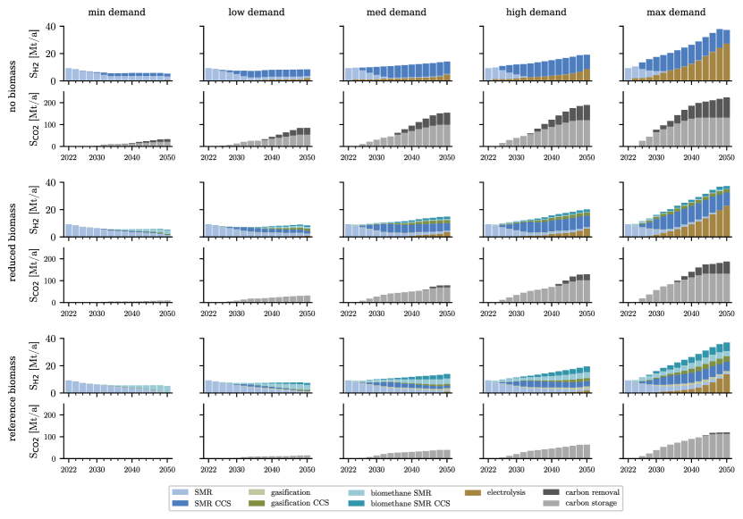
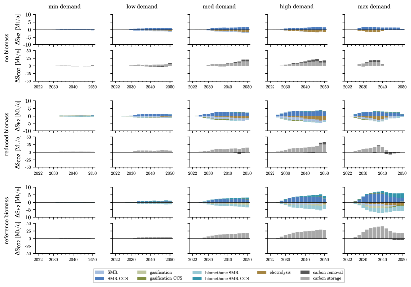
Fig. 4 visualizes the optimal rollout of the \ceH2 production, and \ceCO2 capture and storage capacities across all scenarios. The installed \ceH2 production capacity depends on the expected \ceH2 demand. In the max \ceH2 demand scenario, the \ceH2 production capacity for 2050 is about 7 times higher than in the min \ceH2 demand scenario. In contrast, the \ceH2 production technology mix and the \ceCO2 capture and storage capacities strongly depend on the availability of biomass.
Biomass-based \ceH2 production is identified as the most cost-efficient low-carbon \ceH2 production pathway. By replacing natural gas with biomethane, the SMR process emissions can be reduced by 82 %. Besides installing anaerobic digesters to produce biomethane, no additional investments are required, and existing SMR capacities can continue to be used. Furthermore, the coupling of biomass-based \ceH2 production with CCS results in net-negative emissions, offsetting \ceCO2 emissions that occur at other stages of the supply chain. Therefore, as a first step, scenarios with biomass availability replace natural gas feedstocks with biomethane. With increasing annual decarbonization targets, \ceH2 production is complemented with CCS to reduce process emissions and biomass gasification is deployed. For max \ceH2 demands, the reference biomass potentials are insufficient to fully decarbonize \ceH2 production, and increasing shares of electrolyzers are installed. In addition, investments in \ceCO2 removal technologies are required to offset upstream supply chain emissions from fuel supply chain, plant manufacturing and construction phases (about 6 Mt/a). The same considerations apply for scenarios with reduced biomass availability and medium-max \ceH2 demands, which require between 10-56 Mt/a \ceCO2 removal capacities by 2050 to achieve the net-zero emissions target.
Without biomass feedstock, low-carbon \ceH2 is produced via SMR-CCS from natural gas and electrolysis of renewable electricity, and \ceCO2 removal technologies are installed to eliminate residual emissions and achieve the NZE target. In configurations where the \ceH2 demand is expected to decrease or remain similar to today’s values (i.e., min-low demand scenarios, Fig. 4), \ceH2 is predominantly produced via SMR-CCS, which is associated with larger \ceCO2 emissions, but lower cost compared to electrolysis. Electrolyzer capacities are continuously expanded in scenarios where \ceH2 demand is expected to increase.
Independently of the biomass availability, electrolyzers do not play a role in min-low \ceH2 demands and are only deployed if medium-max demands are expected. Two factors contribute to the increasing deployment of electrolyzers. First, the unit cost of electrolyzers is expected to decrease by 60 % until 2050, making electrolyzers more cost-competitive. Second, the residual emissions of electrolyzers are 4-10 times lower compared to SMR-CCS (0.6-1.6 ton\ceCO2eq./ton\ceH2 vs. 5.9 ton\ceCO2eq./ton\ceH2). Hence, offsetting the residual emissions from electrolysis requires significantly smaller capacities of \ceCO2 removal technologies and \ceCO2 storage. The literature report a wide range of electrolyzer cost estimates. However, even when assuming a very optimistic cost evolution for electrolyzers, where the investment costs are 10 % lower in 2022 and 30 % lower in 2050 with respect to the reference case, electrolyzer capacities remain small and are only deployed at a larger scale in high and max \ceH2 demand scenarios (Section S7).
The \ceCO2 removal technologies are located near the \ceCO2 storage sites to reduce \ceCO2 transport costs. Land requirements for \ceCO2 removal technologies range between 0.2-0.4 km2 [72, 73]. Depending on the scenario the capacity of the \ceCO2 removal technologies range between 6 to 92 Mt/a which translates to 1.2-18 km2 in the best case, and 2.4-37 km2 in the worst case. By far, the largest \ceCO2 removal capacity is installed close to the Northern Lights \ceCO2 storage site in Norway where about 30 Mt/a \ceCO2 are removed from the air each year, requiring an area of 6-12 km2 (about 840-1,680 soccer fields). To provide more context, this corresponds to less than 1 % of the open free available area [74]. In the remaining regions, the \ceCO2 removal capacity is below 8.5 Mt/a (1.7-3.4 km2).
Finally, the regional \ceCO2 storage capacity is limited by the capacity of existing and announced \ceCO2 storage projects, which corresponds to 132 Mt/a [52]. The full \ceCO2 storage potential is used by 2050 if max \ceH2 demands are expected and less than the reference biomass potentials are available for \ceH2 production.
3.2 Hydrogen and carbon dioxide transport networks
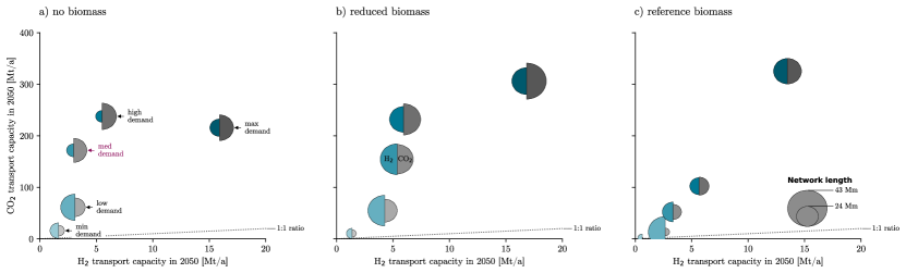
A \ceH2 transport network is required to decouple \ceH2 production and demand. In addition, a \ceCO2 transport network is needed to transport the captured \ceCO2 to the \ceCO2 storage sites. Fig. 5 compares the \ceH2 and \ceCO2 transport networks in 2050 with respect to (i) the network capacity (x and y location of the bubble for \ceH2 and \ceCO2, respectively), and (ii) the network extension (size of the right and left half of the bubble for \ceH2 and \ceCO2, respectively). The capacity of the \ceH2 and \ceCO2 networks is strongly connected to the \ceH2 demands, and in general, the transport volumes and the network capacities increase with increasing \ceH2 demands.
While the \ceH2 network transport capacity is comparable for different levels of biomass, the spatial extension of the network varies greatly. System designs that rely on biomass deploy larger \ceH2 transport infrastructure to overcome the additional spatial constraints imposed by the heterogeneous biomass availabilities and, therefore, more widespread transport infrastructures are required. To enable CCS, the \ceH2 transport infrastructure is accompanied by \ceCO2 transport infrastructure to transport the captured \ceCO2 to the storage sites, and thus, require more extensive \ceCO2 networks. While the capacity of the \ceCO2 networks for reference and reduced biomass are comparable, in case of reduced biomass potentials, the \ceCO2 network covers larger distances to access the available biomass feedstocks and enable the coupling with CCS.
In contrast, system designs that do not rely on biomass produce \ceH2 closer to the demand locations, resulting in smaller, more local \ceH2 transport networks. \ceH2 is largely produced via SMR-CCS from natural gas and electrolysis from renewable electricity, and \ceCO2 removal technologies are installed to offset residual emissions from \ceH2 production and up-stream emissions from plant manufacturing and construction (Fig. 4). In earlier years and for lower demands, \ceH2 is predominantly produced via SMR-CCS. However, for larger \ceH2 demands, SMR-CCS is complemented by increasing shares of electrolyzers, reducing the need for \ceCO2 transport from the \ceH2 production site to the \ceCO2 storage locations (compare infrastructure size for min-low demand and medium-max demand for no biomass in Fig. 5a).
3.3 Levelized cost of hydrogen for different levels of hydrogen demand and biomass availability
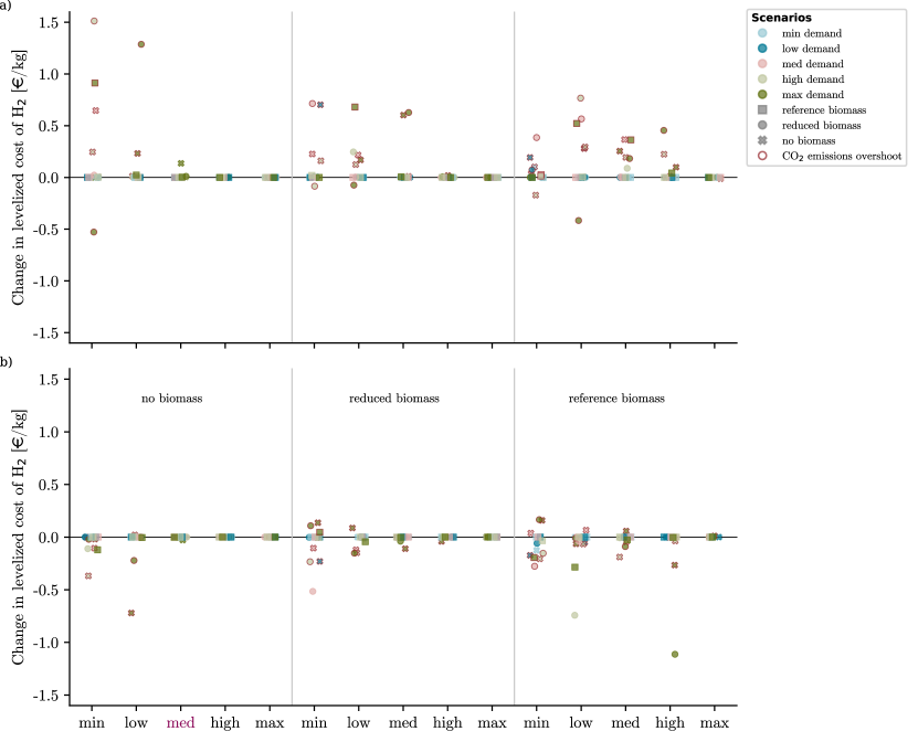
Fig. 6 presents the LCOH (i) for each design scenario (i.e., the system is designed and operated on the same scenario - stacked bars) and (ii) the results of the out-of-sample approach (i.e., the system is designed for one scenario and operated on all other 14 scenarios - markers above each bar). The marker shape and color indicate which out-of-sample scenario the supply chain design is operated on. Furthermore, a red marker edge indicates that the out-of-sample scenario is infeasible, i.e., it is impossible to adjust the system design quickly enough such that the annual \ceCO2 emissions targets are always satisfied.
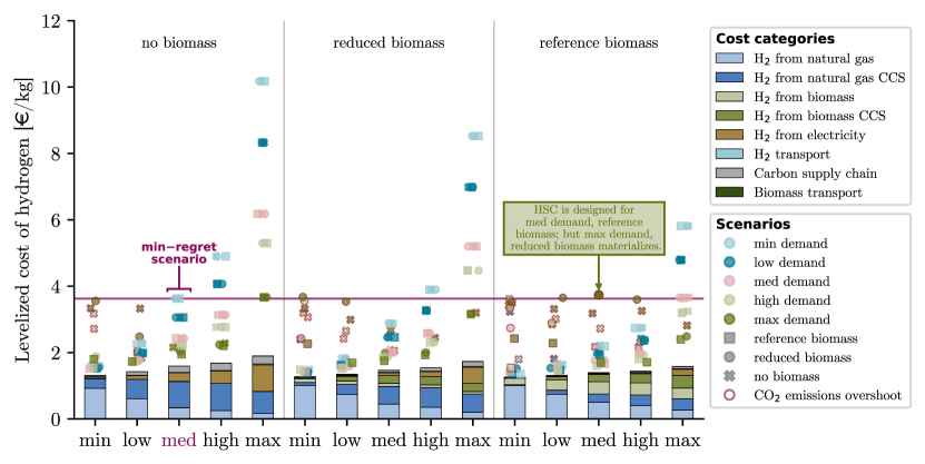
The lowest LCOH is observed for designs with reference biomass. Here, the LCOH is 9-13 % lower compared to design for reduced or no biomass, respectively. Furthermore, we observe a cost increase of up to 44 % with increasing \ceH2 demand. This cost increase is attributed to larger investments in electrolyzers, and \ceCO2 capture, transport, and storage infrastructure, which are not required in scenarios with lower \ceH2 demands. Assuming that a pan-European \ceCO2 transport infrastructure may be deployed independent from the decarbonization of the hard-to-abate industries investigated here, and therefore, \ceCO2 transport infrastructure is available at little to no cost, \ceH2 production capacities from SMR-CCS are expanded (Section S8). This is true, especially for scenarios with reference biomass availability Fig. S6. Nevertheless, the impact of an inexpensive \ceCO2 transport infrastructure is marginal with a LCOH cost reductions below 5 % across scenarios.
If a different scenario materializes than the HSC was initially designed for, the HSC design has to be adjusted to the new conditions and the LCOH increases. Depending on the magnitude of those changes, it may not be possible to adapt the initial supply chain design such that the \ceCO2 emission targets are fulfilled at all times (Section S6). HSC designs where the \ceCO2 emission targets cannot be fulfilled at all times are considered infeasible. These infeasibilities occur predominantly when the \ceH2 demand increases drastically (e.g., instead of min-low demands, high-max demands materialize) or when biomass availability is significantly overestimated during the design phase due to difficulties in scaling up the capacity of low-carbon \ceH2 production and \ceCO2 removal technologies.
The speed at which technology capacities can be expanded is described by the technology expansion rate as a function of the existing technology capacity Section 2.4. The number of infeasible scenarios is lower for more conservative system designs, i.e., systems designed without biomass and for medium to max \ceH2 demands, where larger shares of electrolyzers and \ceCO2 removal technologies allow for a quicker scale-up of the already existing capacities. In contrast, supply chain designs that initially rely largely on biomass-based \ceH2 production technologies are often not able to switch strategies and scale up the capacity of electrolyzers, SMR-CCS, and \ceCO2 removal technologies quickly enough to meet the demand for low-carbon \ceH2. Higher technology expansion rates decrease the number of infeasible scenarios as they allow for a quicker expansion of the existing capacity and, thereby, offer greater flexibility to react and adapt the initial supply chain design to changes (Fig. S2). Nevertheless, the investment strategies remain robust for low and high technology expansion rates, and designing HSCs for medium \ceH2 demands, without biomass remains the minimum-regret strategy.
3.4 Minimum-regret solution
The minimum-regret solution is identified based on two criteria: (1) the solution results in the lowest LCOH in the worst scenario (min-max cost criteria), while (2) meeting the annual \ceCO2 emissions targets (feasibility criteria). Overall, only three out of 15 design scenario designs meet the feasibility criteria of complying with the annual \ceCO2 emissions target at all times and across all out-of-sample scenarios; these are the no biomass scenarios for medium to max \ceH2 demands (Fig. 6). Out of these three scenarios, the designs for medium \ceH2 demands and no biomass is identified as the minimum-regret solution as it results in the lowest LCOH in the worst case (Section 2.5). The minimum-regret solution remains robust for different technology expansion rates (Fig. S2). In the minimum-regret scenario, about 63 % of the \ceH2 demand in 2050 is met via SMR-CCS, and about 34 % via electrolysis from renewable electricity. Depending on the \ceH2 demand of the out-of-sample scenario, the electrolyzer capacity must be expanded by up to 22 Mt/a. While planning for medium demands and reference biomass availability leads to similar LCOH across scenarios, the net-zero emission target for medium-max \ceH2 demands is likely not achieved by 2050 if less biomass is available than expected. Therefore, designing HSCs for medium \ceH2 demands and without the availability of biomass feedstocks is identified as the minimum-regret strategy (Section 3.4).
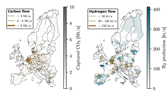
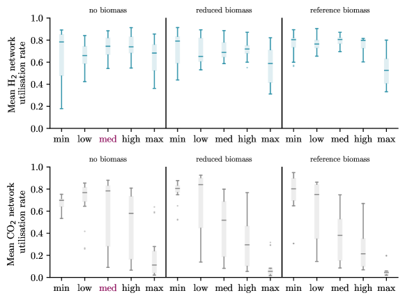
A medium-sized \ceH2 and \ceCO2 transport infrastructure is built (3 Mt/a and 172 Mt/a, respectively, Fig. 7). In particular, the regions of Belgium, Netherlands, and the west of Germany are well connected by \ceH2 and \ceCO2 transport infrastructure. This offers enough flexibility to expand existing capacities without leading to large unused capacities in case smaller \ceH2 demands materialize. Compared to other configurations, the mean network utilization rates remain high (Fig. S3).
4 Discussion
4.1 The role of biomass in decarbonizing \ceH2 production
Biomass-based \ceH2 production is identified as the most cost-efficient low-carbon \ceH2 production technology due to low \ceH2 production cost and \ceCO2 intensities. Especially in the initial phase of the transition, when the capital cost of electrolyzers is still high, biomass-based \ceH2 production dominates the technology mix (Fig. 4 and [75]). This finding is consistent with [76], who investigate the optimal \ceH2 production technology mix under cost uncertainties. In comparison to biomass-based \ceH2 production, the LCOH from electrolysis and renewable electricity is 3-5 times higher, hindering the deployment of electrolyzers at large scales [77]. Even if the projected cost reductions of 2 €/kg\ceH2 can be achieved by 2040 [13], the LCOH from electrolyzers is expected to remain high. Only SMR-CCS can achieve lower \ceH2 production cost than biomass-based technologies (about 1.5 €/kg\ceH2), at the expense of higher process emissions (+2.5-3 kg\ceCO2eq./kg\ceH2). Therefore, the cost-competitiveness of electrolytic \ceH2 is viewed as an unrealistic prospect in the medium-term without appropriate policy support [78].
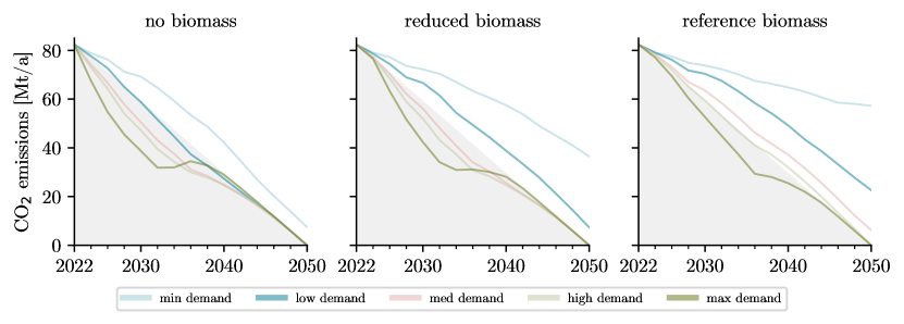
However, the biomass availability is uncertain as multiple sectors compete for it. For instance, biomass can be used as a fuel in the transport sector to decarbonize aviation or heavy-duty transport [79, 29], or it can provide dispatchable, flexible energy in the power sector [80]. While the LCOH is lower in scenarios that rely on biomass in their decarbonization strategy, planning without biomass leads to more robust solutions. Fig. S4 visualizes the annual \ceCO2 emissions for each design scenario. When planning without biomass, most scenarios can eventually achieve a net-zero supply chain design. Only when significantly higher \ceH2 demands materialize than planned (see configurations for min-low demand), the annual \ceCO2 emission targets are overshot during the transition. This observation is robust across the investigated range of technology expansion rates Section S4.
If biomass is included in the technology mix, policymakers must ensure that biomass will be dedicated to low-carbon \ceH2 production. Otherwise, it might not be possible to adapt the decarbonization strategy and scale up alternative \ceH2 production and \ceCO2 removal technologies quickly enough to satisfy the \ceH2 demands in compliance with stricter \ceCO2 emission limits (Fig. 6).
Currently, biomass is predominantly used for heating and cooling (about 75 % in 2018) [81]. However, existing studies indicate that using biomass to decarbonize transport and industry is more attractive than using biomass as a dispatchable, flexible energy source for electricity production [67]. The current bioeconomy strategy of the EU focuses on increasing the sustainability and circularity, but does not provide clear guidelines on the use of biomass [82]. Therefore, we recommend extending existing EU and national bioeconomy strategies to provide clear guidelines on the strategic use of the limited biomass resources; steering the use of biomass to sectors where biomass provides a cost-efficient decarbonization option and which lack alternatives.
4.2 The role of carbon capture, transport, and storage
CO2 capture, transport, and storage (CCTS) infrastructure plays a central role in decarbonizing \ceH2 production. More specifically, when coupling \ceH2 production with CCS, large amounts of \ceCO2 are captured at the production site, transported, and stored underground. When \ceH2 production is based on electrolysis, \ceCO2 removal technologies are installed to remove residual and upstream \ceCO2 emissions. The \ceCO2 removal technologies are typically located close to the \ceCO2 storage sites to reduce transport costs, and thus, require less extensive \ceCO2 transport infrastructure.
For scenarios with large \ceH2 demands and reduced or no biomass, existing and planned \ceCO2 storage sites are fully utilized to achieve net-zero \ceH2 production. A reduced \ceCO2 storage availability would lead to an increased installation of electrolysers. Nevertheless, a minimum of about 7, 11, and 50 Mt\ceCO2/a \ceCO2 removal and storage capacity would be required to offset upstream emissions and realize net-zero \ceH2 production for minimum, medium, and maximum demand, respectively.
The need for CCTS infrastructure is widely recognized [83], and according to the International Association of Oil & Gas Producers (IOGP) [84], Europe requires a minimum of 0.5-1 Gton\ceCO2/a of \ceCO2 storage by 2050 to reach its targets. However, the capacity of existing and currently planned \ceCO2 storage projects in Europe only corresponds to 13-26 % of the storage capacity envisioned by [84]. For reference, the European hard-to-abate industry alone currently emits between 0.7-1 Gton\ceCO2/a. Similar observations are made on a global scale, where only 10 % of the required \ceCO2 storage capacity might be available by 2050, considering the historically observed expansion rates for \ceCO2 storage [85]. This suggests that rapid changes and coordinated efforts are required to enable CCS across sectors and foster the energy transition.
4.3 Implications of a constrained technology expansion
Technology expansion rates are computed based on historically observed annual growth rates, as they do not appear to change significantly over time [86, 47, 68]. Previous studies indicate that energy systems models tend to overestimate the speed at which emerging technologies can penetrate the market [47, 87]. Technology expansion constraints can be used to limit the speed at which the capacity of a technology can be expanded (Section 2.4).
Results indicate that the feasibility and cost of out-of-sample designs strongly depend on the availability of \ceCO2 removal technologies. The reduced investments in \ceCO2 removal technologies in design scenarios that rely on biomass and the coupling with CCS pose challenges when biomass does not become available as planned, especially when larger \ceH2 demands materialize than initially planned for. The results further indicate that planning ahead and investing in sufficient low-carbon \ceH2 production capacities (about 9.6 Mt/a by 2030) is necessary to scale-up low-carbon \ceH2 production and facilitate larger low-carbon \ceH2 demands. Otherwise, the transition might be delayed and the decarbonization targets cannot be met (Fig. 6 and Fig. S4). The planning horizon of 2022-2030 is especially important. Both, the design scenarios for no biomass and low and mean demands fail to achieve the annual emission targets in 2024-2030 because insufficient low-carbon \ceH2 production capacities delay the scale-up of SMR-CCS and electrolyzer capacities, and instead, larger shares of the existing, natural-gas based SMR have to be deployed to meet the increased \ceH2 demands. [88] show that large demands for low-carbon \ceH2 (e.g., induced by high carbon taxation) can stimulate the adoption of low-carbon technologies. Hence, developing a stringent European \ceH2 strategy could promote investments in low-carbon \ceH2 infrastructure and foster its widespread use. The lack of a dedicated \ceH2 and \ceCO2 transport infrastructure [56, 89], as well as uncertainties around material selection and process operation [83] hinder investments in low-carbon \ceH2 and CCTS infrastructure. While the creation of niche markets for low-carbon \ceH2 could accelerate its adoption, this also necessitates a coordinated scale-up of the required low-carbon \ceH2 and CCTS transport infrastructure [56].
5 Conclusion
This work investigates the optimal design and rollout of \ceH2 supply chains (HSCs) to achieve a net-zero European hard-to-abate industry. We determine the optimal technology portfolio of net-zero \ceH2 production technologies while accounting for uncertainties in the evolution of \ceH2 demand and biomass availability. We consider a multi-year time horizon from 2022 to 2050 and include several \ceH2 production pathways, namely water-electrolysis from renewable electricity, SMR from natural gas and biomethane, and biomass gasification. \ceH2 production from biomass and natural gas can be coupled with CCS. In addition, \ceCO2 removal technologies can be installed to remove residual \ceCO2 emissions. Finally, \ceCO2 and biomass transport infrastructures are designed alongside the HSC.
We follow a scenario-based uncertainty quantification approach and define 15 scenarios, considering five levels of \ceH2 demand and three levels of biomass availability. We determine the optimal HSC design for the individual scenarios (design scenarios) and evaluate their performance in case alternative scenarios materialize (out-of-sample approach). Additional investments can be made to adapt the supply chain designs to the new operating conditions. However, these additional investments are limited by technology expansion constraints. The solutions are evaluated and compared based on the levelized cost of \ceH2, and a minimum-regret design is determined based on two criteria: (i) the ability to meet the annual \ceCO2 emissions target and achieve net-zero emissions by 2050, and (ii) the lowest levelized cost of \ceH2 in case the worst-case scenario materializes.
H2 production via SMR-CCS of natural gas and biomethane reforming are the most cost-efficient low-carbon \ceH2 production pathways. Particularly attractive is the coupling of biomass-based \ceH2 production with CCS, a process which achieves a \ceCO2 removal, and can thereby offset emissions at other stages in the supply chain. Investments in electrolyzers are delayed due to high initial capital costs.
To harness the full potential of regionally-constrained biomass and to decouple \ceH2 production and demands, \ceH2 transport infrastructure is required. Furthermore, \ceCO2 capture, transport, and storage infrastructure (CCTS) plays a central role in a low-carbon \ceH2 economy. Especially for larger \ceH2 demands, a pan-European CCTS infrastructure is required to mitigate emissions from \ceH2 production and enable CCS. A minimum \ceCO2 storage capacity of 2.7-50 Mt\ceCO2/a is needed. Hence, a coordinated effort on a European level is required to accelerate the development and deployment of CCTS.
In general, the LCOH is 9 %-13 % lower for configurations that include biomass in their decarbonization strategy. However, a strategy relying on biomass is not robust if biomass availability is reduced. In this case, it is often impossible to adapt the system design and scale up alternative low-carbon \ceH2 production technologies to meet the \ceH2 demand and the decarbonization targets. In contrast, planning without biomass leads to more robust supply chains.
We also find that planning for medium \ceH2 demands and installing a sufficient \ceH2 production capacity (about 9.6 Mt/a by 2030) is required to facilitate the scale-up of existing low-carbon \ceH2 production capacities to accommodate larger \ceH2 demands. Otherwise, the scale-up of the low-carbon \ceH2 production capacity might be delayed, ultimately resulting in a failure to achieve the annual \ceCO2 emissions targets, even if technology expansion rates are high.
A comprehensive European \ceH2 and bioenergy strategy could help navigate these large uncertainties by delineating clear directives on (i) the envisioned applications of \ceH2 and (ii) the role of biomass in the energy transition. Dedicating further research on the role of low-carbon \ceH2 in decarbonizing the selected hard-to-abate industries and identifying no-regret applications can reduce uncertainty regarding future levels of low-carbon \ceH2 demand and guide policymakers. However, if the large uncertainty surrounding the future demand for low-carbon \ceH2 pertains, this may further delay the scale-up of low-carbon HSCs.
Overlooking the importance of CCTS infrastructure can hinder the transition and jeopardize the realization of climate goals. \ceH2 and \ceCO2 transport infrastructure is required independently of the low-carbon \ceH2 demand. Fostering investments in regional \ceH2 and \ceCO2 transport infrastructure that can be expanded if larger low-carbon \ceH2 demands materialize can support a successful transition to net-zero. Incentivizing investments in low-carbon \ceH2 production capacities can further reduce the risks first-movers face (slow market dynamics, high low-carbon \ceH2 production costs, lack of transport infrastructure) and facilitate the scale-up of low-carbon \ceH2 markets.
Finally, although biomass-based \ceH2 production is lower in cost, including biomass in the decarbonization strategy can impose risks if these biomass feedstocks are not made available. Therefore, planning without biomass feedstocks is identified as the minimum-regret strategy. Extending the EU bioenergy strategy and providing clear directives on the sectors that will get access to the limited biomass potentials can guide investments in the low-carbon \ceH2 production technologies. Here, additional research can support policymakers in identifying the sectors where biomass plays a key role in the transition to net zero.
Code and data availability
The code and input data to reproduce the results presented in this work is available on Zenodo: https://zenodo.org/doi/10.5281/zenodo.10930801.
Acknowledgments
This work is supported by the Swiss National Science Foundation, grant no. 200021-182529, and the Swiss Federal Office of Energy as part of the SWEET PATHFNDR project.
Supporting Information
Supporting Information Section S1 Input data to the optimization problem
Section S1.1 Energy carrier prices and carbon intensities
The country-specific grid electricity prices and \ceCO2 intensities are taken from [90]. The country-specific natural gas prices are taken from [91]. The yearly evolution of the natural gas prices is estimated following [92]. The regional wet and dry biomass prices are taken from [50]. Finally, the \ceCO2 intensity of natural gas, wet biomass, and dry biomass are taken from [93, 94].
Section S1.2 Conversion and transport technologies
The parameters describing the technology cost of the conversion technologies are described in Tables S1 and S2. The parameters describing the performance of the conversion technologies are reported in Sections Section S1.2 and S4. The capacity factors and capacity limits for renewable energy technologies are taken from [51]. Finally, the techno-economic parameters of the transport technologies are described in Table S4. The transport distances for the transport technologies are approximated by the Haversine distance between the centroids of two neighboring regions.
| Technologies | unit | 2022 | 2025 | 2030 | 2035 | 2040 | 2045 | 2050 |
|---|---|---|---|---|---|---|---|---|
| Electrolysis [1, 95] | €/kW\ceH2 | 1079 | 913 | 747 | 622 | 498 | 456 | 415 |
| SMR [1] | €/kW\ceH2 | 840 | 824 | 809 | 793 | 777 | 761 | 745 |
| SMR-CCS [96] | €/kW\ceH2 | 1551 | 1404 | 1256 | 1237 | 1219 | 1200 | 1182 |
| Gasification [97, 13] | €/kW\ceH2 | 1327 | 1287 | 1247 | 1207 | 1167 | 1128 | 1088 |
| Gasification-CCS [97, 13] | €/kW\ceH2 | 2449 | 2216 | 1983 | 1953 | 1924 | 1895 | 1866 |
| Anaerobic digestion [13, 95] | €/kWbm | 1224 | 1164 | 1103 | 1074 | 1048 | 1019 | 993 |
| Wind onshore [98] | €/kWe | 1353 | 1303 | 1252 | 1217 | 1182 | 1174 | 1165 |
| Wind offshore [98] | €/kWe | 2115 | 2009 | 1903 | 1827 | 1751 | 1732 | 1712 |
| Solar-PV (rooftop) [98] | €/kWe | 1364 | 1156 | 949 | 875 | 800 | 726 | 652 |
| Solar-PV (utility-scale) [98] | €/kWe | 640 | 547 | 455 | 426 | 398 | 381 | 364 |
| \ceCO2 removal [99] | €/(kg\ceCO2/h) | 7139 | 5225 | 3311 | 2816 | 2321 | 2133 | 1945 |
| \ceCO2 storage [100] | €/(kg\ceCO2/h) | 210 | 210 | 210 | 210 | 210 | 210 | 210 |
| Technologies | fix O&M [%] | var O&M [€/kW\ceH2] | Lifetime [years] | Build time [years] |
|---|---|---|---|---|
| Electrolysis [1] | 1.5 | 0 | 10 | 2 |
| SMR [1] | 4.7 | 0 | 25 | 2 |
| SMR-CCS [96] | 3 | 0 | 25 | 2 |
| Gasification [97, 13] | 5 | 0 | 20 | 2 |
| Gasification-CCS [97, 13] | 5 | 0 | 20 | 2 |
| Anaerobic digestion [13, 95] | 6 | 0 €/kWbm | 20 | 2 |
| Wind onshore [98] | 1 | 14€/kWe | 30 | 2 |
| Wind offshore [98] | 2 | 39€/kWe | 30 | 2 |
| Solar-PV (rooftop) [98] | 2 | 12€/kWe | 40 | 2 |
| Solar-PV (utility-scale) [98] | 2 | 8 €/kWe | 40 | 2 |
| \ceCO2 removal [99] | 4 | 0 €/t\ceCO2 | 25 | 2 |
| \ceCO2 storage [100] | 6 | 0 €/t\ceCO2 | 40 | 2 |
| Production technologies | Conversion | Efficiency | \ceCO2 capture | \ceCO2 intensity |
| Electrolysis [96] | e\ceH2 | 0.64 | - | - |
| \arrayrulecolorblack!30SMR [93] | g \ceH2 | 0.77 | - | - |
| \ceH2 e | 0.041 | |||
| SMR-CCS [93] | g \ceH2 | 0.77 | - | |
| \ceH2 e | 0.016 | |||
| Gasification [94] | B \ceH2 | 0.62 | - | - |
| \ceH2 e | -0.093 | |||
| Gasification-CCS [94] | B \ceH2 | 0.62 | - | |
| \ceH2 e | -0.153 | |||
| Anaerobic digestion [94] | b bm | - | - | |
| \ceCO2 capture (retrofit) [93] | \ceH2 \ceH2 | 1 | - | |
| \cee H2 | 0.025 | |||
| \ceCO2 storage [101] | \ceLC \ceLC | 1 | - | -1 |
| \cee \ceLC | ||||
| \arrayrulecolorblack! |
| Transport technologies | Carrier | Investment | O&M | Operation | Lifetime | Build time | \ceCO2 intensity |
|---|---|---|---|---|---|---|---|
| [€/kW] | [%] | [€/(kW km)] | [year] | [year] | [g/(kWh km)] | ||
| \ceH2 truck (gas) [96] | \ceGH2 | 35 | 4 | 5 | 12 | 1 | 5 |
| \ceH2 truck (liquid) [96] | \ceLH2 | 8 | 4 | 12 | 1 | 8 | |
| \ceH2 pipeline [96] | \ceGH2 | 3 | 4 | 0 | 40 | 4 | 0 |
| Dry biomass truck [28] | B | 6 | 4 | 3 | 12 | 1 | 8 |
| \ceCO2 truck (liquid) [101] | \ceLC | (44 + 0.04 ) €/(t/h km) | 4 | 0.5 €/(t km) | 12 | 1 | 7 |
| \ceCO2 pipeline [101] | \ceLC | 3000 €/(t/h km) | 1 | 0 €/(t km) | 45 | 4 | 1.6 1/km |
Section S1.3 Hydrogen and carbon conditioning technologies
Due to its low energy density at ambient temperatures and pressures (2.4 kg/m3 at 25°C and 30 bar), \ceH2 is typically transported as a compressed gas at ambient temperatures and high pressures (25°C, 200-350 bar), or as a liquid (-253°C, 1 bar)[24, 102, 103], requiring the installation of conditioning technologies in the form of \ceH2 compression, liquefaction, and evaporation technologies. Similar considerations apply to \ceCO2, which is therefore typically transported in its liquid form [101]. The conditioning technologies are modeled following [24] and [103]. The techno-economic parameters of the \ceH2 conditioning technologies are reported in [49].
Supporting Information Section S2 Regional hydrogen demand uncertainty
The regional \ceH2 demands for ammonia production, methanol production and refineries are estimated based on a regionally resolved dataset obtained from [104]. The regional \ceH2 demands for steel and cement industry are estimated using the annual emissions dataset published by the European Environmental Agency (EEA). The dataset includes the location and \ceCO2 emissions of European hard-to-abate industrial facilities emitting more than 0.1 Mt of \ceCO2 per year [6]. The emissions data for 2018 is used since the datasets for later years are incomplete. Based on the emissions data for 2018, we can derive the industry-specific \ceCO2 emissions per NUTS2 region in Europe. Assuming that industry-specific emissions are proportional to the production capacity, we can then estimate the regional \ceH2 demand.
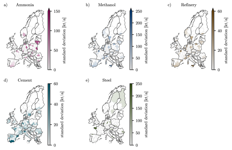
We analyze the variability in the regional \ceH2 demand estimates by comparing their standard deviation. Fig. S1 visualizes the standard deviation for each region and industry in 2050, namely (a) ammonia production, (b) methanol production, (c) refineries, (d) cement production, and (e) steel production. The standard deviation is highest for steel and methanol production, reaching up to 250 kt/a in selected regions in the north-east of Germany and the north-west of France, and up to 280 kt/a in the west of the Netherlands, respectively. The standard deviation for ammonia production is substantially lower, exceeding 100 kt/a only in few select regions in the Netherlands, Germany, Poland and Lithuania. Cement and refineries exhibit the lowest standard deviations. The \ceH2 demands from refineries are expected to decline in future years due to reduced fossil fuel demands. Cement facilities are distributed across the NUTS2 regions and similar in size, resulting in standard deviations around 20 kt/a in most regions.
Supporting Information Section S3 Technology expansion constraints
The capacity of technology at position and time is expressed by . Conversion technologies are installed at nodes and transport technologies can be installed at edges . In each year, the technology capacity can be expanded by . Existing technology capacities that are within their lifetime are expressed by the parameter :
| (2) |
Furthermore, the technology capacity and the capacity expansion are constrained by , and , respectively:
| (3) | ||||
| (4) |
In the out-of-sample approach, the technology capacity expansion is additionally constrained by the technology expansion constraints. These additional constraints are modeled and parameterized following [68, 47]. The technology expansion is limited by the technology expansion rate multiplied by the existing knowledge , which represents the expertise and knowledge of the industry (Eq. 8). In addition, spillover effects from one country to another are considered, assuming a knowledge spillover rate . The unbounded market share and the unbounded capacity addition allow entry into niche markets [68]:
| (5) |
Spillover effects are not included for transport technologies , which connect regions across all nodes:
| (6) |
To avoid unrealistically high spillover effects, the cumulative capacity additions are constrained by the cumulative existing knowledge:
| (7) |
where the existing knowledge is approximated by the previous capacity additions and , and depreciated over time with the knowledge depreciation rate :
| (8) |
Supporting Information Section S4 Sensitivity of the technology expansion constraint parameters
The technology expansion constraint limits the maximum annual growth rate of a technology, and is determined by the technology expansion rate and the existing capacity of a technology. Here, we investigate the impact of different expansion rates on the levelized cost of \ceH2 and compare the results for low expansion rates of 10 %, and high expansion rates of 29 % to the reference case of 20 %. Fig. S2 visualize the change in the levelized cost of \ceH2 (LCOH) for low and high expansion rates with respect to the reference case (Figure 6). A reduction in the technology expansion rate increases the systems inertia making it more difficult to quickly adapt the investment strategy and system cost increase (up to 1.5 €/kg). In contrast, an increase in the technology expansion rate reduces the system inertia, allowing for a quicker implementation of changes in the investment strategy, and a reduction in cost (up to 1.1 €/kg). In general, smaller systems are more sensitive to changes in the expansion rate (e.g., systems designed for min or low \ceH2 demand), whereas the impact of the expansion rate reduces for larger systems, where the maximum annual growth rates remains high due to the larger existing capacities in the system.
Supporting Information Section S5 Network utilization
Fig. S3 shows the utilization rate of the \ceH2 and \ceCO2 transport networks in 2050 across the 15 design scenarios. The network utilization rate in 2050 is computed as the carrier flow divided by the available network capacity, and the variability within each design scenario stems from the 14 out-of-sample scenarios. In general, the mean network utilization rates are lower for higher \ceH2 demands. Supply chains that are initially designed for low \ceH2 demands are characterized by small, local transport networks, which are fully utilized across the out-of-sample scenarios. However, small \ceH2 and \ceCO2 transport capacities prohibit a quick expansion of the transport infrastructure. Instead, alternative \ceH2 production technologies have to be deployed, resulting in substantially higher supply chain costs or a failure to achieve the \ceCO2 emissions targets (Fig. S4).
In contrast, while building large, pan-European \ceH2 and \ceCO2 transport networks offers more flexibility, capacities often remain unused if lower \ceH2 demands materialize, and utilization rates plummet.
Supporting Information Section S6 Annual carbon emissions
Fig. S4 shows the mean annual \ceCO2 emissions in each design scenario. The grey area visualizes the area in which the annual \ceCO2 emissions are lower or equal to the annual \ceCO2 emissions target. In particular, supply chain designs for min and low \ceH2 demands often exceed the annual \ceCO2 emission limits, and low-carbon \ceH2 production has to be substituted with carbonaceous \ceH2 production to satisfy the \ceH2 demand. In contrast, supply chains designed to accommodate larger \ceH2 demands are typically able to adapt their infrastructure quickly enough to achieve the climate targets. Here, we observe that, on average, the HSC emissions stay below the imposed annual \ceCO2 emission targets.
Supporting Information Section S7 Optimistic electrolysis scenario
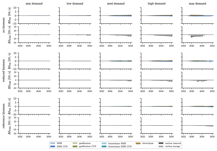
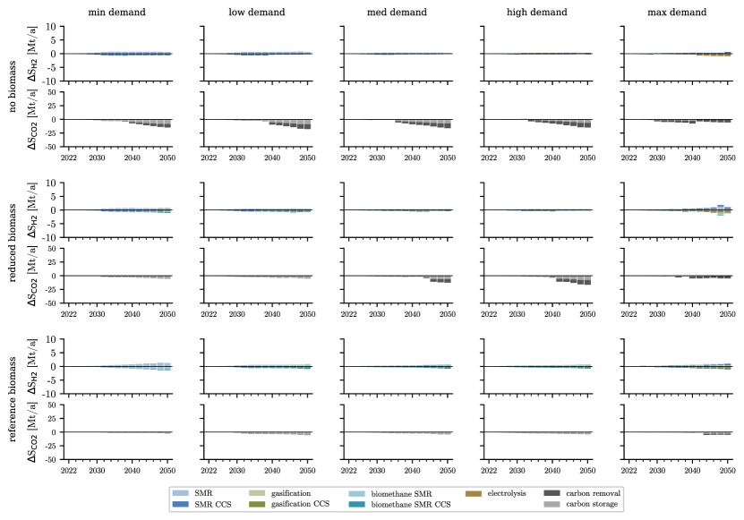
We include an optimistic case for electrolyzers to investigate the impact of our input parameter assumptions on the investment decisions. To this end, the capital investment cost of the electrolyzers is reduced from 1079 €/kW\ceH2 in 2022 and 413 €/kW\ceH2 in 2050 to 985 €/kW\ceH2 in 2022 and 298 €/kW\ceH2 in 2050. In addition, the electrolysis lifetime is increased from 10 to 20 years. Fig. S5 visualizes the changes in the cost-optimal \ceH2 production capacities between 2022 and 2050 compared to the reference case presented in Fig. 4. Even in this optimistic case, the share of electrolyzers does not increase significantly with respect to the reference case, and changes remain below 8 % for the \ceH2 production capacities.
Supporting Information Section S8 Optimistic carbon transport cost scenario
We include an optimistic case for \ceCO2 network to investigate the impact of our input parameter assumptions on the investment decisions. To this end, the capital investment cost of the \ceCO2 trucks and pipelines is reduced to zero, and only the operational costs for \ceCO2 trucks (0.5 €/(t km)) remain. Fig. S6 visualizes the changes in the cost-optimal \ceH2 production capacities between 2022 and 2050 with respect to the reference case presented in Fig. 4. In design scenarios with biomass availability, we observe a shift from low-carbon \ceH2 production from biomass-based \ceH2 production to \ceH2 production from natural gas coupled with CCS. Design scenario designs with med-max \ceH2 demands are affected the most, where biomass-based \ceH2 production capacities reduce by up to 16 % while SMR-CCS capacities increase by up to 26 %. Furthermore, investments in \ceCO2 removal and \ceCO2 storage capacities occur earlier in time, and \ceCO2 storage capacities increase up to 15 % (see reference biomass, max demand). Scenarios that do not include biomass are less affected, and changes remain below 10 % and 15 % for \ceH2 production capacities and \ceCO2 capture and storage capacities, respectively.
Supporting Information Section S9 90 % decarbonization scenario
We include a case with a reduced decarbonization target of 90 % by 2050 to investigate the impact of the net-zero emissions target on our investment decisions. Fig. S7 visualizes the changes in the cost-optimal \ceH2 production capacities between 2022 and 2050 compared to the reference case presented in Fig. 4. We observe that even for a reduced decarbonization target of 90 % by 2050, \ceCO2 capture and storage infrastructure is required. However, on average, \ceCO2 capture and storage capacities reduce by about 24 %.
References
- [1] IEA, The Future of Hydrogen, Tech. rep., International Energy Agency (2019).
-
[2]
M. van der Spek, C. Banet, C. Bauer, P. Gabrielli, W. Goldthorpe, M. Mazzotti, S. T. Munkejord, N. A. Røkke, N. Shah, N. Sunny, D. Sutter, J. M. Trusler, M. Gazzani, Perspective on the hydrogen economy as a pathway to reach net-zero CO 2 emissions in Europe, Energy & Environmental Science 15 (3) (2022) 1034–1077.
doi:10.1039/D1EE02118D.
URL http://xlink.rsc.org/?DOI=D1EE02118D -
[3]
Agora Energiewende and AFRY Management Consulting, No-regret hydrogen: Charting early steps for H2 infrastructure in Europe, Tech. rep., Agora Energiewende and AFRY Management Consulting (2021).
URL https://www.agora-energiewende.de/en/publications/no-regret-hydrogen/ -
[4]
European Commission, REPowerEU: Joint European Action for more affordable, secure and sustainable energy EN, Tech. rep., European Commission (2022).
URL https://eur-lex.europa.eu/legal-content/EN/TXT/?uri=COM%3A2022%3A230%3AFIN&qid=1653033742483 -
[5]
E. E. Agency, Annual European Union greenhouse gas inventory 1990-2021 and inventory report 2023, Publication.
URL https://www.eea.europa.eu/publications/annual-european-union-greenhouse-gas-2 -
[6]
Environmental Energy Agency, Annual European Union greenhouse gas inventory 1990–2020 and inventory report 2022, Tech. rep., Environmental Energy Agency, issue: May (2022).
URL https://www.eea.europa.eu/publications/annual-european-union-greenhouse-gas-1 -
[7]
S. Paltsev, J. Morris, H. Kheshgi, H. Herzog, Hard-to-Abate Sectors: The role of industrial carbon capture and storage (CCS) in emission mitigation, Applied Energy 300 (2021) 117322.
doi:10.1016/j.apenergy.2021.117322.
URL https://www.sciencedirect.com/science/article/pii/S0306261921007327 -
[8]
N. J. Inc, Net-Zero Goals in Chemical Industry Could Shift Energy Demand (Mar. 2022).
URL https://insight.factset.com/net-zero-goals-in-chemical-industry-could-shift-energy-demand -
[9]
European Comission, ’Fit for 55’: delivering the EU’s 2030 Climate Target on the way to climate neutrality, Tech. rep., European Commission, Brussels (2021).
URL https://eur-lex.europa.eu/legal-content/EN/TXT/?uri=CELEX%3A52021DC0550 -
[10]
CertifHy, Hydrogen Certification Schemes.
URL https://www.certifhy.eu/go-labels/ -
[11]
I. E. Agency, Global Hydrogen Review 2023, Tech. rep. (2023).
URL https://iea.blob.core.windows.net/assets/ecdfc3bb-d212-4a4c-9ff7-6ce5b1e19cef/GlobalHydrogenReview2023.pdf -
[12]
Fonseca, Joana, Muron, Matus, Pawelec, Grzegorz, Yovchev, Ivan Petar, Kuhn, Maximilian, Fraile, Daniel, Waciega, Kamila, Azzimonti, Matteo, Brodier, Clémence, Alcade, Isalbel, Antal, Márton Ivan, Marsili, Luca, Pafiti, Antigone, Espitalier-Noel, Marie, Giusti, Niccolò, Durdevic, Dinko, Clean Hydrogen Monitor 2023, Tech. rep. (2023).
URL https://hydrogeneurope.eu/wp-content/uploads/2023/10/Clean_Hydrogen_Monitor_11-2023_DIGITAL.pdf -
[13]
W. Terlouw, D. Peters, K. van der Leun, Gas for Climate. The optimal role for gas in a net zero emissions energy system, Tech. rep., Navigant (2019).
URL https://www.europeanbiogas.eu/wp-content/uploads/2019/11/GfC-study-The-optimal-role-for-gas-in-a-net-zero-emissions-energy-system.pdf - [14] A. Wang, J. J. David Mavins, M. Moultak, M. Schimmel, K. v. d. Leun, D. Peters, M. Buseman, Analysing future demand, supply, and transport of hydrogen, Tech. rep., European Hydrogen Backbone, issue: June (2021).
-
[15]
P. Gabrielli, L. Rosa, M. Gazzani, R. Meys, A. Bardow, M. Mazzotti, G. Sansavini, Net-zero emissions chemical industry in a world of limited resources, One Earth 6 (6) (2023) 682–704.
doi:10.1016/j.oneear.2023.05.006.
URL https://linkinghub.elsevier.com/retrieve/pii/S2590332223002075 -
[16]
European Comission, A hydrogen strategy for a climate-neutral Europe, Tech. rep., European Commission, arXiv: 1011.1669v3 ISBN: 9788578110796 ISSN: 1098-6596 (2020).
URL https://ec.europa.eu/commission/presscorner/home/en -
[17]
European Commission, Clean Planet for all: A European long-term strategic vision for a prosperous, modern, competitive and climate neutral economy, Tech. rep., European Commission (2018).
URL https://eur-lex.europa.eu/legal-content/EN/TXT/?uri=CELEX%3A52018DC0773 -
[18]
J. Cihlar, A. Villar Lejarreta, A. Wang, F. Melgar, J. Jens, P. Rio, Hydrogen generation in Europe: Overview of costs and key benefits, Tech. rep., Publications Office of the european Union, Luxembourg (2020).
URL https://op.europa.eu/en/publication-detail/-/publication/7e4afa7d-d077-11ea-adf7-01aa75ed71a1/language-en -
[19]
B. McWilliams, G. Zachmann, Navigating through hydrogen, Policy Cotnribution, Bruegel (2021).
URL https://www.bruegel.org/2021/04/navigating-through-hydrogen/ -
[20]
F. Neumann, E. Zeyen, M. Victoria, T. Brown, The potential role of a hydrogen network in Europe, Joule (2023) S2542435123002660doi:10.1016/j.joule.2023.06.016.
URL https://linkinghub.elsevier.com/retrieve/pii/S2542435123002660 -
[21]
P. Kotek, B. T. Tóth, A. Selei, Designing a future-proof gas and hydrogen infrastructure for Europe – A modelling-based approach, Energy Policy 180 (2023) 113641.
doi:10.1016/j.enpol.2023.113641.
URL https://www.sciencedirect.com/science/article/pii/S0301421523002264 - [22] J. Ochoa Robles, S. De-León Almaraz, C. Azzaro-Pantel, Design of Experiments for Sensitivity Analysis of a Hydrogen Supply Chain Design Model, Process Integration and Optimization for Sustainability 2 (2) (2018) 95–116, publisher: Process Integration and Optimization for Sustainability. doi:10.1007/s41660-017-0025-y.
- [23] J. O. Robles, C. Azzaro-Pantel, A. Aguilar-Lasserre, Optimization of a hydrogen supply chain network design under demand uncertainty by multi-objective genetic algorithms, Computers & Chemical Engineering 140 (2020) 106853, publisher: Pergamon. doi:10.1016/J.COMPCHEMENG.2020.106853.
-
[24]
P. Gabrielli, F. Charbonnier, A. Guidolin, M. Mazzotti, Enabling low-carbon hydrogen supply chains through use of biomass and carbon capture and storage: A Swiss case study, Applied Energy 275 (2020) 115245.
doi:10.1016/j.apenergy.2020.115245.
URL https://www.sciencedirect.com/science/article/pii/S0306261920307571 -
[25]
C. Bauer, K. Treyer, C. Antonini, J. Bergerson, M. Gazzani, E. Gencer, J. Gibbins, M. Mazzotti, S. T. McCoy, R. McKenna, R. Pietzcker, A. P. Ravikumar, M. C. Romano, F. Ueckerdt, J. Vente, M. van der Spek, On the climate impacts of blue hydrogen production, Sustainable Energy & Fuels 6 (1) (2022) 66–75.
doi:10.1039/D1SE01508G.
URL http://xlink.rsc.org/?DOI=D1SE01508G -
[26]
B. Parkinson, P. Balcombe, J. F. Speirs, A. D. Hawkes, K. Hellgardt, Levelized cost of CO2 mitigation from hydrogen production routes, Energy & Environmental Science 12 (1) (2019) 19–40, publisher: The Royal Society of Chemistry.
doi:10.1039/C8EE02079E.
URL https://pubs.rsc.org/en/content/articlelanding/2019/ee/c8ee02079e -
[27]
T. Nevzorova, V. Kutcherov, Barriers to the wider implementation of biogas as a source of energy: A state-of-the-art review, Energy Strategy Reviews 26 (2019) 100414, publisher: Elsevier Ltd.
doi:10.1016/j.esr.2019.100414.
URL https://doi.org/10.1016/j.esr.2019.100414 -
[28]
V. Schnorf, E. Trutnevyte, G. Bowman, V. Burg, Biomass transport for energy: Cost, energy and CO2 performance of forest wood and manure transport chains in Switzerland, Journal of Cleaner Production 293 (2021) 125971.
doi:10.1016/j.jclepro.2021.125971.
URL https://www.sciencedirect.com/science/article/pii/S0959652621001918 -
[29]
V. Daioglou, B. Wicke, A. P. C. Faaij, D. P. van Vuuren, Competing uses of biomass for energy and chemicals: implications for long-term global CO2 mitigation potential, GCB Bioenergy 7 (6) (2015) 1321–1334, _eprint: https://onlinelibrary.wiley.com/doi/pdf/10.1111/gcbb.12228.
doi:10.1111/gcbb.12228.
URL https://onlinelibrary.wiley.com/doi/abs/10.1111/gcbb.12228 - [30] S. Pfenninger, A. Hawkes, J. Keirstead, Energy systems modeling for twenty-first century energy challenges, Renewable and Sustainable Energy Reviews 33 (2014) 74–86, publisher: Pergamon. doi:10.1016/J.RSER.2014.02.003.
- [31] H. Blanco, J. Leaver, P. E. Dodds, R. Dickinson, D. García-Gusano, D. Iribarren, A. Lind, C. Wang, J. Danebergs, M. Baumann, A taxonomy of models for investigating hydrogen energy systems, Renewable and Sustainable Energy Reviews 167 (2022) 112698, publisher: Pergamon. doi:10.1016/J.RSER.2022.112698.
- [32] X. Yue, S. Pye, J. DeCarolis, F. G. Li, F. Rogan, B. Gallachóir, A review of approaches to uncertainty assessment in energy system optimization models, Energy Strategy Reviews 21 (2018) 204–217, publisher: Elsevier. doi:10.1016/J.ESR.2018.06.003.
-
[33]
X. Wen, M. Jaxa-Rozen, E. Trutnevyte, Hindcasting to inform the development of bottom-up electricity system models: The cases of endogenous demand and technology learning, Applied Energy 340 (2023) 121035, publisher: Elsevier.
doi:10.1016/J.APENERGY.2023.121035.
URL https://linkinghub.elsevier.com/retrieve/pii/S0306261923003999 - [34] J. Koomey, P. Craig, A. Gadgil, D. Lorenzetti, Improving Long-Range Energy Modeling: A Plea for Historical Retrospectives, Source: The Energy Journal 24 (4) (2003) 75–92.
-
[35]
P. P. Craig, A. Gadgil, J. G. Koomey, What Can History Teach Us? A Retrospective Examination of Long-Term Energy Forecasts for the United States*, https://doi.org/10.1146/annurev.energy.27.122001.083425 27 (2003) 83–118, publisher: Annual Reviews 4139 El Camino Way, P.O. Box 10139, Palo Alto, CA 94303-0139, USA.
doi:10.1146/ANNUREV.ENERGY.27.122001.083425.
URL https://www.annualreviews.org/doi/abs/10.1146/annurev.energy.27.122001.083425 - [36] H. A. Linstone, Shaping the Next One Hundred Years: New Methods for Quantitative, Long-Term Policy Analysis: R.J. Lempert, S.W. Popper, and S.C. Bankes, Santa Monica, CA, The RAND Corporation, 2003, Technological Forecasting and Social Change 71 (3) (2004) 305–307, publisher: North-Holland. doi:10.1016/J.TECHFORE.2003.09.006.
-
[37]
J. A. Riera, R. M. Lima, O. M. Knio, A review of hydrogen production and supply chain modeling and optimization, International Journal of Hydrogen Energy 48 (37) (2023) 13731–13755.
doi:10.1016/j.ijhydene.2022.12.242.
URL https://www.sciencedirect.com/science/article/pii/S0360319922060505 - [38] A. Hugo, P. Rutter, S. Pistikopoulos, A. Amorelli, G. Zoia, Hydrogen infrastructure strategic planning using multi-objective optimization, International Journal of Hydrogen Energy 30 (15) (2005) 1523–1534, publisher: Pergamon. doi:10.1016/J.IJHYDENE.2005.04.017.
-
[39]
A. Almansoori, N. Shah, Design and operation of a stochastic hydrogen supply chain network under demand uncertainty, International Journal of Hydrogen Energy 37 (5) (2012) 3965–3977.
doi:10.1016/j.ijhydene.2011.11.091.
URL https://www.sciencedirect.com/science/article/pii/S0360319911025894 - [40] A. O. Bique, L. K. Maia, I. E. Grossmann, E. Zondervan, Design of hydrogen supply chains under demand uncertainty - a case study of passenger transport in Germany, Process Systems Engineering: For a Smooth Energy Transition (2022) 239–260ISBN: 9783110705201. doi:10.1515/9783110705201-009.
-
[41]
G. Yang, Y. Jiang, S. You, Planning and operation of a hydrogen supply chain network based on the off-grid wind-hydrogen coupling system, International Journal of Hydrogen Energy 45 (41) (2020) 20721–20739.
doi:10.1016/j.ijhydene.2020.05.207.
URL https://linkinghub.elsevier.com/retrieve/pii/S0360319920320619 -
[42]
M. Fazli-Khalaf, B. Naderi, M. Mohammadi, M. S. Pishvaee, Design of a sustainable and reliable hydrogen supply chain network under mixed uncertainties: A case study, International Journal of Hydrogen Energy 45 (59) (2020) 34503–34531.
doi:10.1016/j.ijhydene.2020.05.276.
URL https://www.sciencedirect.com/science/article/pii/S0360319920321339 -
[43]
P. Nunes, F. Oliveira, S. Hamacher, A. Almansoori, Design of a hydrogen supply chain with uncertainty, International Journal of Hydrogen Energy 40 (46) (2015) 16408–16418.
doi:10.1016/j.ijhydene.2015.10.015.
URL https://www.sciencedirect.com/science/article/pii/S0360319915303840 -
[44]
J. Lou, Z. Liao, B. Jiang, J. Wang, Y. Yang, Robust optimization of hydrogen network, International Journal of Hydrogen Energy 39 (3) (2014) 1210–1219.
doi:10.1016/j.ijhydene.2013.11.024.
URL https://linkinghub.elsevier.com/retrieve/pii/S0360319913027493 -
[45]
S. De-León Almaraz, C. Azzaro-Pantel, L. Montastruc, S. Domenech, Hydrogen supply chain optimization for deployment scenarios in the Midi-Pyrénées region, France, International Journal of Hydrogen Energy 39 (23) (2014) 11831–11845.
doi:10.1016/j.ijhydene.2014.05.165.
URL https://www.sciencedirect.com/science/article/pii/S0360319914015778 - [46] H. Aissi, C. Bazgan, D. Vanderpooten, Min–max and min–max regret versions of combinatorial optimization problems: A survey, European Journal of Operational Research 197 (2) (2009) 427–438, publisher: North-Holland. doi:10.1016/J.EJOR.2008.09.012.
-
[47]
B. D. Leibowicz, V. Krey, A. Grubler, Representing spatial technology diffusion in an energy system optimization model, Technological Forecasting and Social Change 103 (2016) 350–363.
doi:10.1016/j.techfore.2015.06.001.
URL https://www.sciencedirect.com/science/article/pii/S0040162515001675 -
[48]
eurostat, NUTS - Nomenclature of territorial units for statistics.
URL https://ec.europa.eu/eurostat/web/nuts/overview -
[49]
A. Ganter, P. Gabrielli, G. Sansavini, Near-term infrastructure rollout and investment strategies for net-zero hydrogen supply chains, Renewable and Sustainable Energy Reviews 194 (2024) 114314.
doi:10.1016/j.rser.2024.114314.
URL https://www.sciencedirect.com/science/article/pii/S1364032124000376 -
[50]
C. P. Ruiz, W. Nijs, D. Tarvydas, A. Sgobbi, A. Zucker, R. Pilli, A. Camia, C. Thiel, C. Hoyer-Klick, L. F. Dalla, T. Kober, J. Badger, P. Volker, B. Elbersen, A. Brosowski, D. Thrän, K. Jonsson, ENSPRESO - an open data, EU-28 wide, transparent and coherent database of wind, solar and biomass energy potentials (Jun. 2019).
URL https://publications.jrc.ec.europa.eu/repository/handle/JRC116900 -
[51]
I. Gonzalez-Aparicio, A. Zucker, F. Careri, F. Monforti, T. Huld, J. Badger, EMHIRES dataset: wind and solar power generation, Tech. rep., Joint Research Center (May 2021).
URL https://zenodo.org/record/4803353 - [52] IOGP, CCUS projects in Europe, Tech. rep., IOGP (2023).
-
[53]
P. Ruiz Castello, A. Sgobbi, N. Wouter, C. Thiel, Francesco Dalla Longa, T. Kober, Berien Elbersen, G. Hengeveld, The JRC-EU-TIMES model: bioenergy potentials for EU and neighbouring countries, Publications Office of the European Union, LU, 2015.
URL https://data.europa.eu/doi/10.2790/39014 - [54] N. Scarlat, F. Fahl, J. F. Dallemand, F. Monforti, V. Motola, A spatial analysis of biogas potential from manure in Europe, Renewable and Sustainable Energy Reviews 94 (2018) 915–930, publisher: Pergamon. doi:10.1016/J.RSER.2018.06.035.
-
[55]
Zorg Biogas GmbH, Biomethane transportation container 40" ISO Standard (May 2023).
URL https://zorg-biogas.com/equipment/transportation-methane/methane-transportation-modules -
[56]
D. Schlund, S. Schulte, T. Sprenger, The who’s who of a hydrogen market ramp-up: A stakeholder analysis for Germany, Renewable and Sustainable Energy Reviews 154 (2022) 111810.
doi:10.1016/j.rser.2021.111810.
URL https://www.sciencedirect.com/science/article/pii/S1364032121010789 -
[57]
Material Economics, Industrial Transformation 2050 - Pathways to Net-Zero Emissions from EU Heavy Industry., Focus on Catalysts 2006 (12) (2019) 8.
URL https://materialeconomics.com/publications/industrial-transformation-2050 - [58] S. Luh, S. Budinis, S. Giarola, T. J. Schmidt, A. Hawkes, Long-term development of the industrial sector – Case study about electrification, fuel switching, and CCS in the USA, Computers and Chemical Engineering 133, publisher: Elsevier Ltd (Feb. 2020). doi:10.1016/J.COMPCHEMENG.2019.106602.
-
[59]
A. H. Azadnia, C. McDaid, A. M. Andwari, S. E. Hosseini, Green hydrogen supply chain risk analysis: A european hard-to-abate sectors perspective, Renewable and Sustainable Energy Reviews 182 (2023) 113371.
doi:10.1016/j.rser.2023.113371.
URL https://www.sciencedirect.com/science/article/pii/S1364032123002289 -
[60]
G. Fils, M. Deutsch, 12 Insights on Hydrogen, Tech. rep., Agora Energiewende and AFRY Management Consulting (2021).
URL https://static.agora-energiewende.de/fileadmin/Projekte/2021/2021_11_H2_Insights/A-EW_245_H2_Insights_WEB.pdf -
[61]
M. Wietsche C. Hebling, M. Ragwitz, T. Fleiter, U. Groos, D. Härle, A. Held, M. Jahn, N. Müller, T. Pfeifer, P. Plötz, O. Ranzmeyer, A. Schaadt, F. Sensfuß, T. Smolinka, Eine Wasserstoff-Roadmap für Deutschland, Fraunhofer ISI Fraunhofer ISE (2019) 1–51.
URL https://www.ise.fraunhofer.de/de/presse-und-medien/presseinformationen/2020/fraunhofer-wasserstoff-roadmap.html -
[62]
J. Wachsmuth, A. Aydemir, H. Döscher, J. Eckstein, W. Proganietz, D. E. Francois, D. Scheer, The potential of hydrogen for decarbonising EU industry, Tech. rep., European Parliamentary Research Service Scientific Foresight Unit (STOA) PE 697.199 – December 2021 (2021).
doi:10.2861/271156.
URL https://www.europarl.europa.eu/RegData/etudes/STUD/2021/697199/EPRS_STU(2021)697199_EN.pdf -
[63]
Fuel Cells and Hydrogen Joint Undertaking, Hydrogen Roadmap Europe: A Sustainable Pathway for the European Energy Transition, Tech. rep., Fuel cells and hydrogen joint undertaking, publication Title: Publications Office of the European Union (2019).
doi:10.2843/249013.
URL https://op.europa.eu/en/publication-detail/-/publication/0817d60d-332f-11e9-8d04-01aa75ed71a1 -
[64]
M. Krzywinski, N. Altman, Visualizing samples with box plots, Nature Methods 11 (2) (2014) 119–120, number: 2 Publisher: Nature Publishing Group.
doi:10.1038/nmeth.2813.
URL https://www.nature.com/articles/nmeth.2813 -
[65]
C. Panoutsou, K. Maniatis, Sustainable biomass availability in the EU, to 2050, TAPPI Journal 20 (8) (2021).
doi:10.32964/tj20.8.
URL https://www.concawe.eu/wp-content/uploads/Sustainable-Biomass-Availability-in-the-EU-Part-I-and-II-final-version.pdf - [66] J. Speirs, C. McGlade, R. Slade, Uncertainty in the availability of natural resources: Fossil fuels, critical metals and biomass, Energy Policy 87 (2015) 654–664, publisher: Elsevier. doi:10.1016/J.ENPOL.2015.02.031.
- [67] F. Wu, A. Muller, S. Pfenninger, Strategic uses for ancillary bioenergy in a carbon-neutral and fossil-free 2050 European energy system, Environmental Research Letters 18 (1) (2023). doi:10.1088/1748-9326/aca9e1.
- [68] Jacob Mannhardt, Paolo Gabrielli, Giovanni Sansavini, How to avoid failing the European energy transition.
-
[69]
J. Mannhardt, P. Gabrielli, G. Sansavini, Collaborative and selfish mitigation strategies to tackle energy scarcity: The case of the European gas crisis, iScience 26 (5) (2023) 106750.
doi:10.1016/j.isci.2023.106750.
URL https://www.sciencedirect.com/science/article/pii/S2589004223008271 -
[70]
Gurobi Optimization LLC, Gurobi Optimizer Reference Manual (2022).
URL https://www.gurobi.com -
[71]
European Commission, European Climate Law (2021).
URL https://eur-lex.europa.eu/legal-content/EN/TXT/?uri=CELEX:32021R1119 -
[72]
M. Ozkan, S. P. Nayak, A. D. Ruiz, W. Jiang, Current status and pillars of direct air capture technologies, iScience 25 (4) (2022) 103990.
doi:10.1016/j.isci.2022.103990.
URL https://www.sciencedirect.com/science/article/pii/S2589004222002607 -
[73]
climeworks, Suppport the scale-up of direct air capture (2023).
URL https://climeworks.com/direct-air-capture?utm_source=googleBrand&utm_medium=cpc&utm_campaign=GS-AO-World-en-Brand&utm_term=climeworks&gclid=CjwKCAjwnOipBhBQEiwACyGLugmiA-HDfg1ekwyHv1jZ0nRSwOX7_qYgTdny4vRaR9cosBve55ElJxoCxAQQAvD_BwE -
[74]
Statistics Norway, Land use and land cover (Jul. 2023).
URL https://www.ssb.no/en/natur-og-miljo/areal/statistikk/arealbruk-og-arealressurser - [75] Alissa Ganter, Paolo Gabrielli, Giovanni Sansavini, Optimal infrastructure rollout for net-zero hydrogen supply chains - The impact of spatial resolution.
- [76] B. Lane, J. Reed, B. Shaffer, S. Samuelsen, Forecasting renewable hydrogen production technology shares under cost uncertainty, International Journal of Hydrogen Energy 46 (54) (2021) 27293–27306, publisher: Elsevier Ltd. doi:10.1016/J.IJHYDENE.2021.06.012.
-
[77]
Y. Wang, Y. Pang, H. Xu, A. Martinez, K. S. Chen, PEM Fuel cell and electrolysis cell technologies and hydrogen infrastructure development – a review, Energy & Environmental Science 15 (6) (2022) 2288–2328, publisher: Royal Society of Chemistry.
doi:10.1039/D2EE00790H.
URL https://pubs.rsc.org/en/content/articlelanding/2022/ee/d2ee00790h -
[78]
I. Staffell, D. Scamman, A. Velazquez Abad, P. Balcombe, P. E. Dodds, P. Ekins, N. Shah, K. R. Ward, The role of hydrogen and fuel cells in the global energy system - Energy & Environmental Science (RSC Publishing) (12) (2019) 463–491.
doi:DOI:10.1039/c8ee01157e.
URL https://pubs.rsc.org/en/content/articlelanding/2019/ee/c8ee01157e - [79] V. Becattini, P. Gabrielli, M. Mazzotti, Role of carbon capture, storage, and utilization to enable a Net-Zero-CO2-emissions aviation sector, Industrial and Engineering Chemistry Research 60 (18) (2021) 6848–6862, publisher: American Chemical Society. doi:10.1021/acs.iecr.0c05392.
-
[80]
D. Bogdanov, J. Farfan, K. Sadovskaia, A. Aghahosseini, M. Child, A. Gulagi, A. S. Oyewo, L. de Souza Noel Simas Barbosa, C. Breyer, Radical transformation pathway towards sustainable electricity via evolutionary steps, Nature Communications 10 (1) (2019) 1077, number: 1 Publisher: Nature Publishing Group.
doi:10.1038/s41467-019-08855-1.
URL https://www.nature.com/articles/s41467-019-08855-1 -
[81]
Biomass.
URL https://energy.ec.europa.eu/topics/renewable-energy/bioenergy/biomass_en -
[82]
D.-G. for Research and Innovation (European Commission), Bioeconomy: the European way to use our natural resources : action plan 2018, Publications Office of the European Union, LU, 2018.
URL https://data.europa.eu/doi/10.2777/79401 -
[83]
M. Bui, C. S. Adjiman, A. Bardow, E. J. Anthony, A. Boston, S. Brown, P. S. Fennell, S. Fuss, A. Galindo, L. A. Hackett, J. P. Hallett, H. J. Herzog, G. Jackson, J. Kemper, S. Krevor, G. C. Maitland, M. Matuszewski, I. S. Metcalfe, C. Petit, G. Puxty, J. Reimer, D. M. Reiner, E. S. Rubin, S. A. Scott, N. Shah, B. Smit, J. P. M. Trusler, P. Webley, J. Wilcox, N. M. Dowell, Carbon capture and storage (CCS): the way forward, Energy & Environmental Science 11 (5) (2018) 1062–1176, publisher: The Royal Society of Chemistry.
doi:10.1039/C7EE02342A.
URL https://pubs.rsc.org/en/content/articlelanding/2018/ee/c7ee02342a -
[84]
International Association of Oil & Gas Producers, Press Release (2022).
URL https://iogpeurope.org/news/europe-needs-a-co2-storage-ambition-for-2050/#:~:text=Ahead%20of%20the%202nd,an%20interim%20ambition%20for%202035. -
[85]
E. Martin-Roberts, V. Scott, S. Flude, G. Johnson, R. S. Haszeldine, S. Gilfillan, Carbon capture and storage at the end of a lost decade, One Earth 4 (11) (2021) 1569–1584.
doi:10.1016/j.oneear.2021.10.002.
URL https://linkinghub.elsevier.com/retrieve/pii/S2590332221005418 -
[86]
C. Wilson, Meta-analysis of unit and industry level scaling dynamics in energy technologies and climate change mitigation scenarios, Tech. rep., International Institute for Applied Systems Analysis (IIASA) (2009).
URL https://www.jstor.org/stable/resrep15764.3 -
[87]
C. Bertram, N. Johnson, G. Luderer, K. Riahi, M. Isaac, J. Eom, Carbon lock-in through capital stock inertia associated with weak near-term climate policies, Technological Forecasting and Social Change 90 (2015) 62–72.
doi:10.1016/j.techfore.2013.10.001.
URL https://www.sciencedirect.com/science/article/pii/S004016251300259X -
[88]
Y. Shi, Z. Wei, M. Shahbaz, Y. Zeng, Exploring the dynamics of low-carbon technology diffusion among enterprises: An evolutionary game model on a two-level heterogeneous social network, Energy Economics 101 (2021) 105399.
doi:10.1016/j.eneco.2021.105399.
URL https://www.sciencedirect.com/science/article/pii/S014098832100298X - [89] International Energy Agency (IEA), Technology Perspectives Energy Special Report on Carbon Capture Utilisation and Storage CCUS in clean energy transitions, Tech. rep. (2020).
-
[90]
P. Capros, A. De Vita, A. Florou, M. Kannavou, T. Fotiou, P. Siskos, I. Tsiropoulos, N. Katoufa, I. Mitsios, S. Evangelopoulou, G. Asimakopoulou, T. Kalokyris, L. Paroussos, K. Fragkiadakis, P. Karkatsoulis, L. Höglund-Isaksson, W. Winiwarter, P. Purohit, A. Gómez-Sanabria, P. Rafaj, L. Warnecke, A. Deppermann, M. Gusti, S. Frank, P. Lauri, F. di Fulvio, N. Forsell, Havlík Petr;, P. Witzke, M. Kesting, EU Reference Scenario 2020, Tech. rep., European Commission, iSBN: 9789276393566 (2021).
URL https://op.europa.eu/s/shWr -
[91]
eurostat, Gas prices components for non-household consumers - annual data (2022).
URL https://ec.europa.eu/eurostat/databrowser/view/NRG_PC_203_C$DEFAULTVIEW/default/table -
[92]
International Energy Agency, Renewable Energy Market Update - Outlook for 2023 and 2024, Tech. rep., International Energy Agency (2023).
URL https://iea.blob.core.windows.net/assets/63c14514-6833-4cd8-ac53-f9918c2e4cd9/RenewableEnergyMarketUpdate_June2023.pdf -
[93]
C. Antonini, K. Treyer, A. Streb, M. van der Spek, C. Bauer, M. Mazzotti, Hydrogen production from natural gas and biomethane with carbon capture and storage – A techno-environmental analysis, Sustainable Energy & Fuels 4 (6) (2020) 2967–2986.
doi:10.1039/D0SE00222D.
URL http://xlink.rsc.org/?DOI=D0SE00222D -
[94]
C. Antonini, K. Treyer, E. Moioli, C. Bauer, T. J. Schildhauer, M. Mazzotti, Hydrogen from wood gasification with CCS – a techno-environmental analysis of production and use as transport fuel, Sustainable Energy & Fuels 5 (10) (2021) 2602–2621.
doi:10.1039/D0SE01637C.
URL http://xlink.rsc.org/?DOI=D0SE01637C -
[95]
M. Victoria, E. Zeyen, T. Brown, Speed of technological transformations required in Europe to achieve different climate goals, Joule 6 (5) (2022) 1066–1086, arXiv: 2109.09563 Publisher: Elsevier Inc.
doi:10.1016/j.joule.2022.04.016.
URL https://doi.org/10.1016/j.joule.2022.04.016 -
[96]
International Energy Agency (IEA), IEA G20 Hydrogen report: Assumption, Tech. rep., International Energy Agency.
URL https://iea.blob.core.windows.net/assets/29b027e5-fefc-47df-aed0-456b1bb38844/IEA-The-Future-of-Hydrogen-Assumptions-Annex_CORR.pdf -
[97]
M. Binder, Kraussler, Michael, Kuba, Matthias, Luisser, Markus, Hydrogen from biomass gasification, Tech. rep., IEA Bioenergy, iSBN: 9781910154595 (2018).
URL https://www.ieabioenergy.com/wp-content/uploads/2019/01/Wasserstoffstudie_IEA-final.pdf - [98] A. Kättlitz, M. C. Cavarretta, N. Buyuk, O. Lebois, P. Boersma, Scenario Building Guidelines, Tech. rep., entsog and entso (2021).
-
[99]
M. Fasihi, O. Efimova, C. Breyer, Techno-economic assessment of CO2 direct air capture plants, Journal of Cleaner Production 224 (2019) 957–980.
doi:10.1016/j.jclepro.2019.03.086.
URL https://linkinghub.elsevier.com/retrieve/pii/S0959652619307772 -
[100]
Zero Emissions Platform, The Costs of CO2 Storage, Tech. rep., Zero Emissions Platform (2011).
URL www.zeroemissionsplatform.eu/library/publication/168-zep-cost-report-storage.html -
[101]
V. Becattini, P. Gabrielli, C. Antonini, J. Campos, A. Acquilino, G. Sansavini, M. Mazzotti, Carbon dioxide capture, transport and storage supply chains: Optimal economic and environmental performance of infrastructure rollout, International Journal of Greenhouse Gas Control 117 (2022) 103635.
doi:10.1016/j.ijggc.2022.103635.
URL https://www.sciencedirect.com/science/article/pii/S1750583622000548 -
[102]
S. Krasae-in, J. H. Stang, P. Neksa, Development of large-scale hydrogen liquefaction processes from 1898 to 2009, International Journal of Hydrogen Energy 35 (10) (2010) 4524–4533, publisher: Elsevier Ltd.
doi:10.1016/j.ijhydene.2010.02.109.
URL http://dx.doi.org/10.1016/j.ijhydene.2010.02.109 -
[103]
M. Reuß, T. Grube, M. Robinius, P. Preuster, P. Wasserscheid, D. Stolten, Seasonal storage and alternative carriers: A flexible hydrogen supply chain model, Applied Energy 200 (2017) 290–302, publisher: Elsevier Ltd.
doi:10.1016/j.apenergy.2017.05.050.
URL https://linkinghub.elsevier.com/retrieve/pii/S0306261917305457 -
[104]
Fuel cells and hydrogen observatory, Hydrogen supply and demand, Tech. rep., FCH, issue: September (2021).
URL https://www.fchobservatory.eu/sites/default/files/reports/Chapter2HydrogenSupplyandDemand2021.pdf