The vertical-velocity skewness in the inertial sublayer of turbulent wall flows

Abstract

We provide empirical evidence that within the inertial sub layer of adiabatic turbulent flows over smooth walls, the skewness of the vertical velocity component $Sk_{w}$ displays universal behaviour, being constant and constrained within the range $Sk_{w}\approx 0.1-0.16$, regardless of flow configuration and Reynolds number. A theoretical model is proposed to explain the observed behaviour, including the observed range of variations of $Sk_{w}$. The model clarifies why $Sk_{w}$ cannot be predicted from down-gradient closure approximations routinely employed in meteorological and climate models whereby $Sk_{w}$ impacts cloud formation and dispersion processes. The model also offers an alternative and implementable approach.

z

I Introduction

Much of the effort devoted to the study of adiabatic and hydrodynamically smooth wall turbulence has focused on the characterization of velocity statistics within the so-called logarithmic or inertial sublayer (ISL). The Attached Eddy Model (AEM), which is probably the most cited model for ISL-turbulence, predicts that first and second order velocity statistics can be described as [1, 2, 3]:

$$\overline{u}^{+}=\frac{1}{\kappa}\log\left({z^{+}}\right)+A;~{}\sigma_{u}^{2+}=A_{u}-B_{u}\log\left(\frac{z}{\delta}\right);$$ (1)

and, a less studied outcome, $\sigma_{w}^{2+}=A_{w}^{2}$, where $u$ and $w$ are the longitudinal and wall-normal velocity component, respectively; $z$ is the wall normal coordinate; $\sigma_{u}=\sqrt{\overline{u^{\prime 2}}}$ and $\sigma_{w}=\sqrt{\overline{w^{\prime 2}}}$ are the standard deviation of $u$ and $w$ respectively; primes identify fluctuations due to turbulence around the mean; the overline represents averaging over coordinates of statistical homogeneity; the plus index indicates classical inner scaling whereby velocities and lengths are normalized with the friction velocity $u_{*}$ and viscous length scale $\nu/u_{*}$, respectively, with $\nu$ being the kinematic viscosity of the fluid; $\delta$ is the outer length scale of the flow; $\kappa$, $A$, $A_{u}$, $A_{w}$, $B_{u}$ are coefficients that are thought to attain asymptotic constant values at very large Reynolds numbers $Re_{\tau}=u_{*}\delta/\nu$ [4, 2, 5]. The AEM has been extended to velocity moments of any order as well as cross-correlations between different velocity components thereby providing an expanded picture of ISL flow statistics [6]. However, convincing empirical support for the aforementioned theoretical predictions is limited to the statistics of $u$ [2, 4, 7, 8, 9]. In contrast, the statistics of $w$ have been much less reported and investigated, partly because of the technical difficulties associated with accurately measuring $w$ in the near wall region of laboratory flows at high $Re_{\tau}$. As a result, theoretical predictions of $w-$statistics have received mixed support from the literature [10, 11, 12] and higher order moments of $w^{\prime}$ are rarely reported but with few notable exceptions [13, 14, 15, 16, 17]. We argue that this overlook contributed to hide a universal property of ISL turbulence, which is herein reported and discussed. The aim of this letter is to demonstrate that the skewness of $w^{\prime}$, $Sk_{w}=\overline{w^{\prime 3}}/\sigma_{w}^{3}$, is constant (i.e. $z-$independent) and robust to variations in $Re_{\tau}$ within the ISL. Moreover, a theoretical model that explains this observed behaviour and links $Sk_{w}$ to established turbulence constants is proposed, leading to satisfactory predictions. Finally, we note that the asymmetry in the probability density function of $w^{\prime}$, as quantified by $Sk_{w}$, cannot be accounted for with gradient-diffusion representations routinely employed in meteorological and climate models [18]. Rectifying this limitation is of significance because $Sk_{w}$ was shown to impact cloud formation [19, 20, 21] and dispersion processes [22, 23, 24, 25].

Figure 1 reports the variations of $Sk_{w}$ with normalized wall-normal distance ($z/\delta$) using data from Direct Numerical Simulations (DNS) [26] and laboratory experiments [17] pertaining to flat plate turbulent boundary layers (TBLs). Data from experiments on uniform [27] and weakly non-uniform turbulent open channel flows [15, 16], whereby accurate measurements of $w$ are available are also included. This data refers to flows within the low to medium range of $Re_{\tau}$ (Table 1). A reference value of $Sk_{w}=0.1$ is added to the figure as often reported for atmospheric surface layers in adiabatic conditions across multiple heights and surface cover [28]. This value is representative of flows at extremely high $Re_{\tau}$. A region of constant $Sk_{w}$ weakly varying between 0.1 and 0.16 (here weakly means that variations are much smaller than those displayed by $Sk_{w}$ over the entire flow domain) is evident in all profiles within the range $2.6\sqrt{Re_{\tau}}\nu/u_{*}$ up to $0.15-0.25\delta$, which is often associated with the ISL [29, 30, 11]. This finding is remarkable given the large differences in $Re_{\tau}$, measurement techniques and experimental facilities used. In what follows, a theoretical model that predicts and explains such a behaviour is provided.

II Theory

To explain the observed behaviour of $Sk_{w}$, a stationary and planar homogeneous incompressible flow in the absence of subsidence is considered for $\overline{w^{\prime 3}}$. For these conditions, the model can be derived from the Reynolds averaged Navier-Stokes equations and is given as [31, 32]

$$\frac{\partial\overline{w^{\prime 3}}}{\partial t}=0 =+\overbrace{3\sigma_{w}^{2}\frac{\partial\sigma_{w}^{2}}{\partial z}}^{{\rm Source/Sink}}-\overbrace{\frac{\partial\overline{w^{\prime}w^{\prime 3}}}{\partial z}}^{{\rm Turbulent~{}transport}}$$ (2)

$$-\underbrace{3\left(\overline{w^{\prime}w^{\prime}\frac{\partial p^{\prime}}{\partial z}}\right)}_{{\rm Pressure~{}velocity~{}destruction}}-\underbrace{2\nu\left(3\overline{w^{\prime}\frac{\partial w^{\prime}}{\partial z}\frac{\partial w^{\prime}}{\partial z}}\right)}_{{\rm Viscous~{}destruction}},$$

where $t$ is time and $p^{\prime}$ is the pressure deviation from the mean or hydrostatic state normalized by a constant fluid density $\rho$.

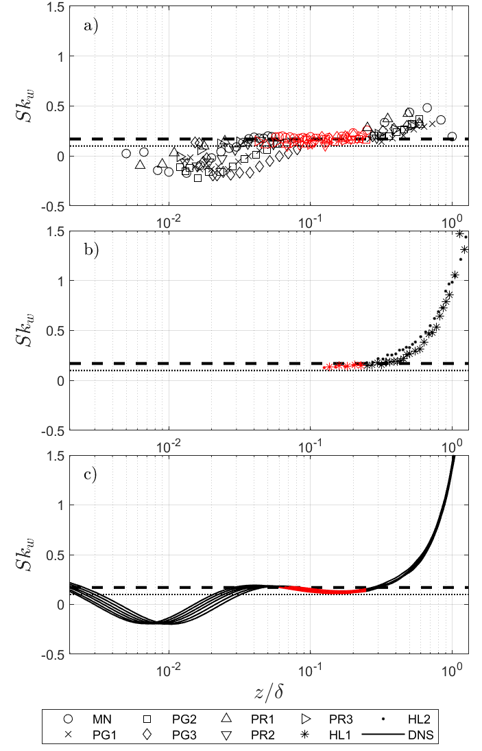
Figure 1: Variation of the vertical velocity skewness $Sk_{w}$ with normalized wall-normal distance $z/\delta$. The dashed line is $Sk_{w}=0.16$ and the dotted line is $Sk_{w}=0.10$. Data sources and references are summarized in Table 1. Red symbols and lines identify the ISL range. For HL1 and HL2, near wall data are not reported due to issues with velocity measurements associated with an excessive sampling volume of the x-probe employed in the experiments [17].

The first two terms on the right-hand side of equation 2 arise from inertial effects or convective acceleration, the third and fourth terms arise due to interactions between $w^{\prime}w^{\prime}$ and the forces acting on a fluid element ($p^{\prime}/\rho$ and viscous stresses). A quasi-normal approximation for the fourth moment is used [33] so that $FF_{w}=\overline{w^{\prime 4}}/(\sigma_{w})^{4}=3+a$ and the overall inertial term simplifies to

$$-\frac{\partial\overline{w^{\prime 4}}}{\partial z}+3\sigma_{w}^{2}\frac{\partial\sigma_{w}^{2}}{\partial z}=-(3+2a)\sigma_{w}^{2}\frac{\partial\sigma_{w}^{2}}{\partial z},$$ (3)

where $a\neq 0$ allows for deviations from Gaussian tails ($a=0$ recovers a Gaussian flatness factor). Usage of a quasi-Gaussian approximation to close a fourth (and even) moment budget makes no statement on the asymmetry (or odd moments) of the $w^{\prime}$ probability density function, only that large-scale intermittency is near-Gaussian, a finding well supported in the literature [34] and many phenomenological approaches [6]. Models for the pressure velocity and viscous destruction terms are now needed to integrate equation 2. A return to isotropy (or Rotta) model [35] given by

$$-2\overline{w^{\prime}\frac{\partial p^{\prime}}{\partial z}}=\frac{C_{R}}{\tau}\left(\frac{\overline{q}}{3}-\sigma_{w}^{2}\right),$$ (4)

may be used to derive an expression for the pressure-velocity destruction term in in equation 2 where $q=u^{\prime}u^{\prime}+v^{\prime}v^{\prime}+w^{\prime}w^{\prime}$ is twice the instantaneous turbulent kinetic energy, $\overline{q}=2K$, $K$ is the averaged turbulent kinetic energy, $v^{\prime}$ is the lateral turbulent velocity, and $C_{R}=1.8$ is a well established constant, the Rotta constant [36]. The $C_{R}$ relates the so-called relaxation time $\tau=\overline{q}/\overline{\epsilon}$ to the time it takes for isotropy to be attained at the finest scales, where $\overline{\epsilon}$ is the mean turbulent kinetic energy dissipation rate. In deriving such an extension, the non-averaged form of equation 4 is first multiplied by $(3/2)w^{\prime}$ and then averaged to yield

$$-3\left(\overline{w^{\prime}w^{\prime}\frac{\partial p^{\prime}}{\partial z}}\right)=\frac{3}{2}\frac{C_{R}}{\tau_{s}}\left(\frac{\overline{w^{\prime}q}}{3}-\overline{w^{\prime}w^{\prime 2}}\right),$$ (5)

where $\tau_{s}$ is another decorrelation time that can differ from $\tau$. The difference between $\tau$ and $\tau_{s}$ arises because when multiplying the instantaneous form of equation 4 by $w^{\prime}$ to arrive at the instantaneous form of equation 5, the correlation between $q$ and $w^{\prime}$ must be considered after averaging. While expected to be small relative to the pressure-velocity interaction term, the viscous destruction contribution is herein retained and represented as [32]

$$-2\nu\left(3\overline{w^{\prime}\frac{\partial w^{\prime}}{\partial z}\frac{\partial w^{\prime}}{\partial z}}\right)=-2\overline{\epsilon^{\prime}w^{\prime}}=-c_{2}\frac{\overline{w^{\prime}q}}{\tau_{s}},$$ (6)

where $c_{2}$ is a similarity constant, and $\epsilon^{\prime}\sim q/\tau_{s}$ is the fluctuating dissipation rate around $\overline{\epsilon}$. Inserting these approximations into equation 2 yields,

$$\overline{w^{\prime 3}}=-\frac{2}{3}\frac{(3+2a)\tau_{s}\sigma_{w}^{2}}{C_{R}}\frac{\partial\sigma_{w}^{2}}{\partial z}+\overline{w^{\prime}q}\left(\frac{1}{3}-\frac{2c_{2}}{3C_{R}}\right).$$ (7)

Table 1: Overview of smooth-wall boundary layer experiments (OC = open channel/flumes, WT = wind tunnel) and direct numerical simulation* in Figure 1. The $Re_{\tau}=\delta u_{*}/\nu$ is the friction Reynolds number, $B_{u}$ and $A_{w}$ were computed from data using AEM. For the DNS, the highest and lowest $Re_{\tau}$ are shown given the small variability in $B_{u}$ (0.91-0.94) and $A_{w}$ (1.15-1.17). The computed $Sk_{w}$ using equation 11 is also presented.

Source	Data set	Flow	$Re_{\tau}$	$B_{u}$	$A_{w}$	$Sk_{w}$
Manes et al. [15]	MN	OC	2160	0.58	1.06	0.11
Sillero et al. [26]	DNS*		1307	0.85	1.15	0.13
			2000	0.86	1.17	0.12
Heisel et al. [17]	HL1	WT	3800	0.85	0.96	0.21
	HL2	WT	4700	0.63	1.00	0.15
Poggi et al. [27]	PG1	OC	1232	0.73	0.90	0.23
	PG2	OC	1071	0.78	1.02	0.17
	PG3	OC	845	1.03	0.90	0.33
Peruzzi et al. [16]	PR1	OC	2240	0.78	1.12	0.13
	PR2	OC	999	0.63	1.06	0.12
	PR3	OC	1886	0.85	1.06	0.16

A model for $\overline{w^{\prime}q}$ is further needed to infer $Sk_{w}$. To arrive at this model, the $K$ budget for the same flow conditions leading to equation 2 are employed. When mechanical production is balanced by $\overline{\epsilon}$ as common to the ISL, the $K$ budget leads to two outcomes [37]

$$u_{*}^{2}\frac{\partial\overline{u}}{\partial z}-\overline{\epsilon}=0;~{}~{}-\frac{1}{2}\frac{\partial\overline{w^{\prime}q}}{\partial z}=0.$$ (8)

The height-independence of $\overline{w^{\prime}q}$ is suggestive that it must be controlled by local conditions and a down-gradient approximation is justified given by [37]

$$-\frac{1}{2}\overline{w^{\prime}q}=\kappa zu_{*}\frac{\partial K}{\partial z}.$$ (9)

The model in equation 9 has received experimental support even for rough-wall turbulent boundary layers and across a wide range of Reynolds numbers and surface roughness values [37]. Noting that $K\approx\sigma_{u}^{2}$ yields

$$\overline{w^{\prime 3}}= -\frac{2}{3}\left[K_{t,w}\frac{\partial\sigma_{w}^{2}}{\partial z}+K_{t,u}\frac{\partial\sigma_{u}^{2}}{\partial z}\right];$$ (10)

$$K_{t,w}= \frac{(3+2a)\tau_{s}\sigma_{w}^{2}}{C_{R}};~{}K_{t,u}=\kappa zu_{*}\left(1-\frac{2c_{2}}{C_{R}}\right),$$

where $K_{t,w}$ and $K_{t,u}$ are eddy viscosity terms. These two eddy viscosity values become comparable in magnitude when setting $\tau_{s}=\kappa z/u_{*}$ (i.e. following classical ISL scaling) and $C_{R}=1.8$ - its accepted value [36] as expected in the ISL. To determine $\partial{\sigma_{w}^{2}}/{\partial z}$, the mean vertical velocity equation is considered for the same idealized flow conditions as equation 2. This consideration results in ${\partial\sigma_{w}^{2}}/{\partial z}=-({1}/{\rho})({\partial\overline{P}}/{\partial z})-g$, where $g$ is the gravitational acceleration. When $\overline{P}=-\rho gz$ (i.e. hydrostatic), $\partial\sigma_{w}^{2}/\partial z=0$ or $A_{w}$ is constant in $z$ within the ISL. That is, the AEM requires $\overline{P}$ to be hydrostatic. However, the AEM precludes a $\partial\sigma_{u}^{2}/\partial z=0$ in the ISL. In fact, the AEM predicts a $\partial\sigma_{u}^{2}/\partial z=-u_{*}^{2}B_{u}/z$ when the $Re_{\tau}$ is very large as expected in the ISL of an adiabatic atmosphere. Inserting this estimate into equation 10, setting $u_{*}=\sigma_{w}/A_{w}$ and momentarily ignoring $\partial{\sigma_{w}^{2}}/{\partial z}$ relative to $\partial\sigma_{u}^{2}/\partial z$ as a simplification consistent with the AEM, leads to

$$Sk_{w}=\frac{\overline{w^{\prime 3}}}{\sigma_{w}^{3}}=\frac{2}{3}\left(1-\frac{2c_{2}}{C_{R}}\right)\frac{\kappa B_{u}}{A_{w}^{3}}.$$ (11)

This equation is the sought outcome. The term $2c_{2}/C_{R}$ reflects the relative importance of the pressure-velocity to viscous destruction terms. Pressure-velocity destruction effects are far more efficient than viscous effects supporting the argument that $2c_{2}/C_{R}<<1$ at very high $Re_{\tau}$ [38] such as the atmosphere. This implies that the numerical value of $Sk_{w}$, as obtained from equation 11, depends on three well established phenomenological constants, namely $\kappa$, $A_{w}$, and $B_{u}$ [8, 3, 9], which, in turn, may depend weakly on $Re_{\tau}$ and the flow type. Equation 11 is also insensitive to the choices made for $\tau_{s}$, because the AEM requires $\partial\sigma_{w}^{2}/\partial z=0$.

III Discussion and Conclusion

Equation 11 demonstrates two inter-related aspects about $Sk_{w}$ in the ISL: (i) why $Sk_{w}$ is positive and constant with $z$, and (ii) why conventional gradient diffusion approximations fail to predict $\overline{w^{\prime 3}}$ from $\partial\sigma_{w}^{2}/\partial z$. Regarding the first, equation 11 predicts that $Sk_{w}>0$ consistent with the paradigm that ejective eddy motions ($w^{\prime}>0,u^{\prime}<0$) are more significant in momentum transfer than sweeping motions ($w^{\prime}<0,u^{\prime}>0$) within the ISL. This assertion is supported by numerous experiments and simulations [39, 40, 17] and adds further confidence in the physics associated with the derivation of equation 11. Moreover, values of the constants in equation 11 for flat plate turbulent boundary layers (TBL) at $Re_{\tau}\to\infty$ correspond to $\kappa=0.39$, $A_{w}=1.33$, and $B_{u}=1.26$ [2, 9]. Upon further setting $c_{2}=0.1$ and $C_{R}=1.8$ (conventional values), leads to $Sk_{w}=0.12$. This estimate compares well with $Sk_{w}=0.1$ reported for the ISL in the adiabatic atmosphere [28, 41]. At the low to moderate $Re_{\tau}$ pertaining to the experiments and DNS associated with Figure 1, equation 11 cannot be used to estimate $Sk_{w}$ using asymptotic values of $A_{w}$ and $B_{u}$. However, Figure 1 shows that these flows attain similar (i.e. slightly higher) and reasonably z-independent values of $Sk_{w}$. To explain this behaviour, the DNS data are used as they allow exploring theoretical predictions offered by equation 10 with reliable estimations of $\sigma_{w}^{2}$ and $\sigma_{u}^{2}$ vertical gradients. Figure 2 indicates that, for mostof the ISL, the first term on the right hand side of the equation is an order of magnitude smaller than the second and can be discarded as predicted by the AEM and advocated in the proposed theory. Predictions of $Sk_{w}$ obtained from the second term are excellent in the ISL and resemble the observed z-independent behaviour. Besides providing further confidence on the proposed theory, this result indicates that, since $K_{t,u}$ is directly proportional to $z$, $\partial\sigma_{u}^{2}/\partial z$ must overall scale as $\sim 1/z$, as predicted by the AEM. Hence, we argue that the AEM represents a reasonable approximation provided $B_{u}$ and $A_{w}$ are adjusted to accommodate for low $Re_{\tau}$ effects. As shown in Figure 3, this is the case for both DNS and laboratory data.

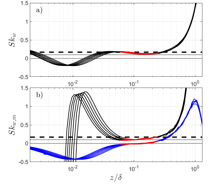
Figure 2: Panel a): Variation of the vertical velocity skewness $Sk_{w}$ with normalized wall-normal distance $z/\delta$ from DNS [26]; panel b): $Sk_{w,m}$ is the modelled vertical velocity skewness using the first term (blue line) and second term (black line) on the right hand side of equation 10 both scaled with $\sigma_{w}^{3}$. In both panels, red lines identify the ISL range. The dashed line is $Sk_{w}=0.16$ and the dotted line is $Sk_{w}=0.10$

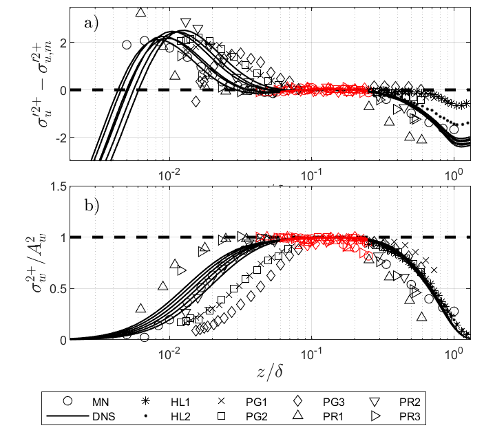
Figure 3: Panel a): difference between $\sigma_{u}^{2+}$ and estimations obtained from the AEM, $\sigma_{u,m}^{2+}=A_{u}-B_{u}\log(z/\delta)$ using values of $A_{u}$ and $B_{u}$ obtained from regression of data within the ISL range (identified by red symbols and lines); panel b): non dimensional vertical velocity variance $\sigma_{w}^{2}$ normalized with $A_{w}$ obtained from data fitting within the ISL vs wall-normal distance $z/\delta$. Data sources and references are summarized in Table 1.

For the DNS, appropriate values of $A_{w}$(=1.15-1.17) and $B_{u}$(=0.85-0.86) were estimated by fitting the AEM to the available data for all available $Re_{\tau}$. The constant $\kappa$=0.39 was assumed as reported in the literature [4, 16]. When inserting these choices of $A_{w}$ and $B_{u}$ from the DNS into equation 11, the computed $Sk_{w}=0.13$, which is close to reported values in Figure 1c. The same approach was used for all laboratory studies. When combining all the runs together (wind tunnel and open channel experiments), ensemble-averaged $A_{w}=1.01\pm 0.074$ and the ensemble-averaged $B_{u}=0.76\pm 0.14$ were obtained across runs within an experiment and across experiments. These values result in an ensemble-averaged $Sk_{w}=0.18\pm 0.07$ and agrees with the measurements reported in Figure 1.

This analysis and Figure 1 suggest that $Sk_{w}$ for DNS and experiments is higher than $0.12$, as estimated for $Re_{\tau}\to\infty$. This is probably because of deviations in the ISL variance statistics from their asymptotic constants in Equation 1. The effects of such deviations on $Sk_{w}$ are however modest because, while low-$Re_{\tau}$ flows are characterized by values of $A_{w}$ and $B_{u}$ that are significantly lower than their counterparts at $Re_{\tau}\to\infty$ (i.e. $A_{w}=1.33$, and $B_{u}=1.26$, see Table 1), equation 11 indicates that $Sk_{w}$ is dictated by the ratio $B_{u}/A_{w}^{3}$, and hence the effect of such deviations are in good part compensated.

Regarding the second feature, equation 10 offers an explanation as to why conventional down-gradient closure models with eddy viscosity $K_{t}\propto\overline{q}l_{m}$ ($l_{m}$ is a ’master’ mixing length) expressed in general index notation ($[x_{1},x_{2},x_{3}]=[x,y,z]$ and $[u^{\prime}_{1},u^{\prime}_{2},u^{\prime}_{3}]=[u^{\prime},v^{\prime},w^{\prime}]$) as [42]

$$\overline{u_{i}^{\prime}u_{j}^{\prime}u_{k}^{\prime}}=-K_{t}\left[\frac{\partial\overline{u_{i}^{\prime}u_{j}^{\prime}}}{\partial x_{k}}+\frac{\partial\overline{u_{i}^{\prime}u_{k}^{\prime}}}{\partial x_{j}}+\frac{\partial\overline{u_{j}^{\prime}u_{k}^{\prime}}}{\partial x_{i}}\right]$$ (12)

spectacularly fail when $i=j=k=3$ and when $A_{w}$ is approximately constant in the ISL (as in the AEM). Yet, the derived equation here also offers a rectification based on the AEM. This rectification accommodates the role of finite $\partial\sigma_{u}^{2}/\partial z$ on $\overline{w^{\prime 3}}$ that cannot arise from equation 12. While studies of the failure of gradient-diffusion models have a long tradition in turbulence research [43], the mode of failure these studies identify differ from the standard one offered here. The classical failure of the so-called gradient diffusion phenomenology is the lack of accommodation of flux transport terms [44, 43]. The origin of the failure of equation 12 here is attributed to a return-to-isotropy mechanism (i.e. pressure-velocity destruction) that requires a model for the vertical transport of $K$, which is dominated by $\sigma_{u}^{2}$ [37]. To be clear, equation 2 does maintain the turbulent flux transport term of $\overline{w^{\prime 3}}$ through $\partial\overline{w^{\prime 4}}/\partial z$, which is modeled using a quasi-normal approximation. However, this term is not the main reason why equation 12 fails. In fact, the final $Sk_{w}$ expression is independent of $a$ when $A_{w}$ is constant (as in AEM) irrespective of whether $a=0$ or not. What was earlier assumed was $a$ not vary appreciably with $z$ within the ISL.

In conclusion, this letter demonstrates that, within the ISL of turbulent and adiabatic smooth wall flows, $Sk_{w}$ attain z-independent values that are predictable from well known turbulence constants relating to the AEM. This behavior is reported for a variety of different wall flows and is independent of variations in $Re_{\tau}$, hence universal and robust.

References

- Townsend [1976] A. Townsend, The Structure of Turbulent Shear Flow (Cambridge University Press, 1976).
- Smits et al. [2011] A. J. Smits, B. J. McKeon, and I. Marusic, High-Reynolds number wall turbulence, Annual Review of Fluid Mechanics 43 (2011).
- Marusic and Monty [2019] I. Marusic and J. P. Monty, Attached eddy model of wall turbulence, Annual Review of Fluid Mechanics 51, 49 (2019).
- Marusic et al. [2013] I. Marusic, J. P. Monty, M. Hultmark, and A. J. Smits, On the logarithmic region in wall turbulence, Journal of Fluid Mechanics 716, R3 (2013).
- Stevens et al. [2014] R. J. Stevens, M. Wilczek, and C. Meneveau, Large-eddy simulation study of the logarithmic law for second-and higher-order moments in turbulent wall-bounded flow, Journal of Fluid Mechanics 757, 888 (2014).
- Woodcock and Marusic [2015] J. Woodcock and I. Marusic, The statistical behaviour of attached eddies, Physics of Fluids 27 (2015).
- Meneveau and Marusic [2013] C. Meneveau and I. Marusic, Generalized logarithmic law for high-order moments in turbulent boundary layers, Journal of Fluid Mechanics 719, R1 (2013).
- Banerjee and Katul [2013] T. Banerjee and G. G. Katul, Logarithmic scaling in the longitudinal velocity variance explained by a spectral budget, Physiscs of Fluids 25, 125106 (2013).
- Huang and Katul [2022] K. Y. Huang and G. G. Katul, Profiles of high-order moments of longitudinal velocity explained by the random sweeping decorrelation hypothesis, Physical Review Fluids 7, 044603 (2022).
- Morrill-Winter et al. [2015] C. Morrill-Winter, J. Klewicki, R. Baidya, and I. Marusic, Temporally optimized spanwise vorticity sensor measurements in turbulent boundary layers, Experiments in Fluids 56, 216 (2015).
- Örlü et al. [2017] R. Örlü, T. Fiorini, A. Segalini, G. Bellani, A. Talamelli, and P. H. Alfredsson, Reynolds stress scaling in pipe flow turbulence—first results from CICLoPE, Philosophical Transactions of the Royal Society A: Mathematical, Physical and Engineering Sciences 375, 20160187 (2017).
- Zhao and Smits [2007] R. Zhao and A. J. Smits, Scaling of the wall-normal turbulence component in high-Reynolds-number pipe flow, Journal of Fluid Mechanics 576, 457 (2007).
- Flack et al. [2007] K. Flack, M. Schultz, and J. Connelly, Examination of a critical roughness height for outer layer similarity, Physics of Fluids 19 (2007).
- Schultz and Flack [2007] M. Schultz and K. Flack, The rough-wall turbulent boundary layer from the hydraulically smooth to the fully rough regime, Journal of Fluid Mechanics 580, 381 (2007).
- Manes et al. [2011] C. Manes, D. Poggi, and L. Ridolfi, Turbulent boundary layers over permeable walls: scaling and near-wall structure, Journal of Fluid Mechanics 687, 141 (2011).
- Peruzzi et al. [2020] C. Peruzzi, D. Poggi, L. Ridolfi, and C. Manes, On the scaling of large-scale structures in smooth-bed turbulent open-channel flows, Journal of Fluid Mechanics 889, A1 (2020).
- Heisel et al. [2020] M. Heisel, G. G. Katul, M. Chamecki, and M. Guala, Velocity asymmetry and turbulent transport closure in smooth-and rough-wall boundary layers, Physical Review Fluids 5, 104605 (2020).
- Mellor and Yamada [1982] G. L. Mellor and T. Yamada, Development of a turbulence closure model for geophysical fluid problems, Reviews of Geophysics 20, 851 (1982).
- Bogenschutz et al. [2012] P. Bogenschutz, A. Gettelman, H. Morrison, V. Larson, D. Schanen, N. Meyer, and C. Craig, Unified parameterization of the planetary boundary layer and shallow convection with a higher-order turbulence closure in the Community Atmosphere Model: Single-column experiments, Geoscientific Model Development 5, 1407 (2012).
- Huang et al. [2020] M. Huang, H. Xiao, M. Wang, and J. D. Fast, Assessing CLUBB PDF closure assumptions for a continental shallow-to-deep convective transition case over multiple spatial scales, Journal of Advances in Modeling Earth Systems 12, e2020MS002145 (2020).
- Li et al. [2022] T. Li, M. Wang, Z. Guo, B. Yang, Y. Xu, X. Han, and J. Sun, An updated CLUBB PDF closure scheme to improve low cloud simulation in CAM6, Journal of Advances in Modeling Earth Systems 14, e2022MS003127 (2022).
- Bærentsen and Berkowicz [1984] J. H. Bærentsen and R. Berkowicz, Monte Carlo simulation of plume dispersion in the convective boundary layer, Atmospheric Environment 18, 701 (1984).
- Luhar and Britter [1989] A. K. Luhar and R. E. Britter, A random walk model for dispersion in inhomogeneous turbulence in a convective boundary layer, Atmospheric Environment (1967) 23, 1911 (1989).
- Wyngaard and Weil [1991] J. C. Wyngaard and J. C. Weil, Transport asymmetry in skewed turbulence, Physics of Fluids A: Fluid Dynamics 3, 155 (1991).
- Maurizi and Tampieri [1999] A. Maurizi and F. Tampieri, Velocity probability density functions in lagrangian dispersion models for inhomogeneous turbulence, Atmospheric Environment 33, 281 (1999).
- Sillero et al. [2013] J. A. Sillero, J. Jiménez, and R. D. Moser, One-point statistics for turbulent wall-bounded flows at Reynolds numbers up to + = 2000, Physics of Fluids 25 (2013).
- Poggi et al. [2002] D. Poggi, A. Porporato, and L. Ridolfi, An experimental contribution to near-wall measurements by means of a special laser doppler anemometry technique, Experiments in Fluids 32, 366 (2002).
- Chiba [1978] O. Chiba, Stability dependence of the vertical wind velocity skewness in the atmospheric surface layer, Journal of the Meteorological Society of Japan. Ser. II 56, 140 (1978).
- Zhou and Klewicki [2015] A. Zhou and J. Klewicki, Properties of the streamwise velocity fluctuations in the inertial layer of turbulent boundary layers and their connection to self-similar mean dynamics, International Journal of Heat and Fluid Flow 51, 372 (2015).
- Örlü et al. [2016] R. Örlü, A. Segalini, J. Klewicki, and P. H. Alfredsson, High-order generalisation of the diagnostic scaling for turbulent boundary layers, Journal of Turbulence 17, 664 (2016).
- Canuto et al. [1994] V. Canuto, F. Minotti, C. Ronchi, R. Ypma, and O. Zeman, Second-order closure pbl model with new third-order moments: Comparison with les data, Journal of the Atmospheric Sciences 51, 1605 (1994).
- Zeman and Lumley [1976] O. Zeman and J. L. Lumley, Modeling buoyancy driven mixed layers, Journal of Atmospheric Sciences 33, 1974 (1976).
- André et al. [1976] J. André, G. De Moor, P. Lacarrere, and R. Du Vachat, Turbulence approximation for inhomogeneous flows: Part I. the clipping approximation, Journal of Atmospheric Sciences 33, 476 (1976).
- Meneveau [1991] C. Meneveau, Analysis of turbulence in the orthonormal wavelet representation, Journal of Fluid Mechanics 232, 469 (1991).
- Rotta [1951] J. Rotta, Statistische Theorie nichthomogener Turbulenz, Zeitschrift für Physik 129, 547 (1951).
- Bou-Zeid et al. [2018] E. Bou-Zeid, X. Gao, C. Ansorge, and G. G. Katul, On the role of return to isotropy in wall-bounded turbulent flows with buoyancy, Journal of Fluid Mechanics 856, 61 (2018).
- Lopez and García [1999] F. Lopez and M. H. García, Wall similarity in turbulent open-channel flow, Journal of Engineering Mechanics 125, 789 (1999).
- Katul et al. [2013] G. G. Katul, A. Porporato, C. Manes, and C. Meneveau, Co-spectrum and mean velocity in turbulent boundary layers, Physics of Fluids 25 (2013).
- Nakagawa and Nezu [1977] H. Nakagawa and I. Nezu, Prediction of the contributions to the Reynolds stress from bursting events in open-channel flows, Journal of Fluid Mechanics 80, 99 (1977).
- Raupach [1981] M. Raupach, Conditional statistics of Reynolds stress in rough-wall and smooth-wall turbulent boundary layers, Journal of Fluid Mechanics 108, 363 (1981).
- Barskov et al. [2023] K. Barskov, D. Chechin, I. Drozd, A. Artamonov, A. Pashkin, A. Gavrikov, M. Varentsov, V. Stepanenko, and I. Repina, Relationships between second and third moments in the surface layer under different stratification over grassland and urban landscapes, Boundary-Layer Meteorology 187, 311 (2023).
- Launder et al. [1975] B. E. Launder, G. J. Reece, and W. Rodi, Progress in the development of a Reynolds-stress turbulence closure, Journal of Fluid Mechanics 68, 537 (1975).
- Corrsin [1975] S. Corrsin, Limitations of gradient transport models in random walks and in turbulence, in Advances in Geophysics, Vol. 18 (Elsevier, 1975) pp. 25–60.
- Cava et al. [2006] D. Cava, G. Katul, A. Scrimieri, D. Poggi, A. Cescatti, and U. Giostra, Buoyancy and the sensible heat flux budget within dense canopies, Boundary-Layer Meteorology 118, 217 (2006).