PLANAR GRAPHS IN BLOWUPS OF FANS

We show that every $n$-vertex planar graph is contained in the graph obtained from a fan by blowing up each vertex by a complete graph of order $O(\sqrt{n}\log^{2}n)$. Equivalently, every $n$-vertex planar graph $G$ has a set $X$ of $O(\sqrt{n}\log^{2}n)$ vertices such that $G-X$ has bandwidth $O(\sqrt{n}\log^{2}n)$. This result holds in the more general setting of graphs contained in the strong product of a bounded treewidth graph and a path, which includes bounded genus graphs, graphs excluding a fixed apex graph as a minor, and $k$-planar graphs for fixed $k$. These results are obtained using two ingredients. The first is a new local sparsification lemma, which shows that every $n$-vertex planar graph $G$ has a set of $O((n\log n)/D)$ vertices whose removal results in a graph with local density at most $D$. The second is a generalization of a method of Feige and Rao, that relates bandwidth and local density using volume-preserving Euclidean embeddings.

1 Introduction

This paper studies the global structure of planar graphs and more general graph classes, through the lens of graph blowups. Here, the $b$-blowup of a graph $H$ is the graph obtained by replacing each vertex $v$ of $H$ with a complete graph $K_{v}$ of order $b$ and replacing each edge $vw$ of $H$ with a complete bipartite graph with parts $V(K_{v})$ and $V(K_{w})$, as illustrated in Figure 1. We consider the following question: What is the simplest family of graphs $\mathcal{H}$ such that, for each $n$-vertex planar graph $G$, there is a graph $H\in\mathcal{H}$ such that $G$ is contained in a $\tilde{O}(\sqrt{n})$-blowup of $H$, where $\tilde{O}$ notation hides $\operatorname{polylog}(n)$ terms? We show that one can take $\mathcal{H}$ to be the class of fans, where a fan is a graph consisting of a path $P$ plus one center vertex adjacent to every vertex in $P$.

Theorem 1.

For each $n\in\mathbb{N}_{1}$ there exists a $O(\sqrt{n}\log^{2}n)$-blowup of a fan that contains every $n$-vertex planar graph.

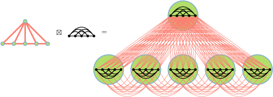
Figure 1: The $5$-blowup of a $6$-vertex fan.

The blowup factor in this result is close to best possible. The $k$-blowup of a graph $H$ with treewidth $t$ has treewidth at most $k(t+1)-1$. Since there are $n$-vertex planar graphs of treewidth $\Omega(\sqrt{n})$ (such as the $\sqrt{n}\times\sqrt{n}$ grid), any result like Theorem 1 that finds all planar graphs in blowups of bounded treewidth graphs must have blowups of size $\Omega(\sqrt{n})$ (and fans have treewidth 2, in fact pathwidth 2). Several other aspects of Theorem 1 are best-possible. These are discussed in Section 1.2, after a review of related previous work.

Theorem 1 can be restated in terms of the following classical graph parameter. Let $G$ be a graph. For an ordering $v_{1},\ldots,v_{n}$ of $V(G)$, let the bandwidth $\leavevmode\color[rgb]{0.76,0.13,0.28}\operatorname{bw}_{G}(v_{1},\ldots,v_{n}):=\max(\{|j-i|:v_{i}v_{j}\in E(G)\}\cup\{0\})$. The bandwidth of $G$ is $\leavevmode\color[rgb]{0.76,0.13,0.28}\operatorname{bw}(G):=\min\{\operatorname{bw}_{G}(v_{1},\ldots,v_{n}):\text{$v_{1},\ldots,v_{n}$ is an ordering of $V(G)$}\}$. See [12, 49, 2, 8, 45, 9, 32] for a handful of important references on this topic. It is well known that bandwidth is closely related to blowups of paths [25, 8]. Indeed, Theorems 1 and 2 are equivalent, where $X$ is the set of vertices mapped to the center of the fan; see Lemmas 10 and 12 for a proof.

Theorem 2.

Every $n$-vertex planar graph $G$ has a set $X$ of $O(\sqrt{n}\log^{2}n)$ vertices such that $G-X$ has bandwidth $O(\sqrt{n}\log^{2}n)$.

We in fact prove several generalizations of Theorem 2 that (a) study the tradeoff between $|X|$ and the bandwidth of $G-X$, and (b) consider more general graph classes than planar graphs.

It follows from the Lipton–Tarjan Planar Separator Theorem that every $n$-vertex planar graph $G$ satisfies $\operatorname{tw}(G)\leqslant\operatorname{pw}(G)\in O(\sqrt{n})$ (see [6]). It is also well known that $\operatorname{pw}(G)\leqslant\operatorname{bw}(G)$ (since if $\operatorname{bw}_{G}(v_{1},\dots,v_{n})\leqslant k$ then $\{v_{1},\dots,v_{k+1}\},\{v_{2},\dots,v_{k+2}\},\dots,\{v_{n-k},\dots,v_{n}\}$ is a path-decomposition of $G$ of width $k$). However, $\operatorname{bw}(G)\in\tilde{O}(\sqrt{n})$ is a much stronger property than $\operatorname{pw}(G)\in\tilde{O}(\sqrt{n})$. Indeed, bandwidth can be $\Omega(n/\log n)$ for very simple graphs, such as $n$-vertex complete binary trees. This highlights the strength of Theorem 2. In fact, Theorem 2 is tight (up to $\operatorname{polylog}$ factors) even for complete binary trees. For a complete binary tree $T$ on $n$ vertices, $\operatorname{bw}(T)\in\Omega(n/\log n)$ since the root of $T$ is within distance $\log n$ of all vertices. For any set $X\subseteq V(T)$, $T$ contains a complete binary tree with $\Omega(n/|X|)$ vertices that avoids $X$, so $\operatorname{bw}(T-X)\geqslant\Omega((n/|X|)/\log(n/|X|))$. Thus, $\operatorname{bw}(T-X)\in\tilde{\Omega}(\sqrt{n})$ for any set $X\subseteq V(T)$ of size $\tilde{O}(\sqrt{n})$.

1.1 Previous Results

As summarized in Table 1, we now compare Theorem 1 with results from the literature, starting with the celebrated Planar Separator Theorem due to Lipton and Tarjan [42], which states that any $n$-vertex planar graph $G$ contains a set $X$ of $O(\sqrt{n})$ vertices such that each component of $G-X$ has at most $n/2$ vertices. This theorem quickly leads to results about the blowup structure of planar graphs. By applying it recursively, it shows that any $n$-vertex planar graph $G$ is contained in a graph that can be obtained from the closure of a tree of height $O(\log n)$ by blowing up the nodes of depth $i$ into cliques of size $O(\sqrt{n/2^{i}})$. (This observation is made by Babai et al. [4] to show that there is a universal graph with $O(n^{3/2})$ edges and that contains all $n$-vertex planar graphs.) By applying it differently, Lipton and Tarjan [43] show that $G$ is contained in a graph obtained from a star by blowing up the root into a clique of size $n^{1-a}$ and blowing up each leaf into a clique of size $O(n^{2a})$. These two structural results have had an enormous number of applications for algorithms, data structures, and combinatorial results on planar graphs. The second result, with $a=n^{1/3}$, shows that $G$ is contained in a $O(n^{2/3})$-blowup of a star. Dvořák and Wood [28] use the second result recursively (with the size of the separator fixed at $c\sqrt{n}$ even for subproblems of size less than $n$) to show that $G$ is contained in the $O(\sqrt{n})$-blowup of the closure of a tree of height $O(\log\log n)$. That is, $G$ is contained in the $O(\sqrt{n})$-blowup of a graph of treedepth $O(\log\log n)$. The same method, with the size of the separator fixed at $cn^{1/2+\epsilon}$ shows that $G$ is contained in an $O(n^{1/2+\epsilon})$-blowup of a graph of treedepth $O(1/\epsilon)$ [28].

Table 1: Results on $b$-blowups of a graph $H$ that contain every $n$-vertex graph $G$ from graph class $\mathcal{G}$.

class $\mathcal{G}$	$H$	lower bound on $b$		upper bound on $b$
planar	tree	$\Omega(n^{2/3})$	[41]	$O(n^{2/3})$	[43]
	$\operatorname{tw}\leqslant 2$	$\Omega(\sqrt{n})$		$O(\sqrt{n})$	[17]
	fan	$\Omega(\sqrt{n})$		$O(\sqrt{n}\log^{2}n)$	Theorem 1
	$\operatorname{tw}\leqslant 3$	$\Omega(\operatorname{tw}(G))$		$\operatorname{tw}(G)+1$	[36]
	$\operatorname{td}\leqslant c\log\log n$	$\Omega(\sqrt{n})$	[28]	$O(\sqrt{n})$	[28]
	$\operatorname{td}\leqslant c/\epsilon$	$\Omega(n^{1/2+\epsilon})$	[28]	$O(n^{1/2+\epsilon})$	[28]
max-degree $\Delta$	tree	$\Omega(\Delta\cdot\operatorname{tw}(G))$	[51]	$O(\Delta\cdot\operatorname{tw}(G))$	[16, 51, 20]
$K_{t}$-minor-free	$\operatorname{tw}\leqslant t-2$	$\Omega(\sqrt{n})$		$O(\sqrt{tn})$	[36]
$K_{t}$-minor-free	$\operatorname{tw}\leqslant t-2$			$\operatorname{tw}(G)+1$	[36]
$K_{t}$-minor-free	$\operatorname{tw}\leqslant 4$	$\Omega(t\sqrt{n})$	[3]	$O_{t}(\sqrt{n})$	[17]
	fan	$\Omega(\sqrt{gn})$	[34]	$O(\sqrt{gn}+\sqrt{n}\log^{2}n)$	Theorem 3
Euler genus $g$	$\operatorname{tw}\leqslant 2$	$\Omega(\sqrt{gn})$	[34]	$O((g+1)\sqrt{n})$	[17]
	$\operatorname{tw}\leqslant 3$			$2(g+1)(\operatorname{tw}(G)+1)$	[36]
$k$-planar	fan	$\Omega(\sqrt{kn})$	[22]	$O(k^{5/4}\sqrt{n}\log^{2}n)$	Theorem 4
$(g,k)$-planar	fan	$\Omega(\sqrt{gkn})$	[22]	$O(g^{1/2}k^{5/4}\sqrt{n}\log^{2}n)$	Theorem 5
$K_{3,t}$-minor-free	$\operatorname{tw}\leqslant 2$	$\Omega(\sqrt{tn})$		$O(t\sqrt{n})$	[17]
$A$-minor-free	fan	$\Omega(\sqrt{n})$		$O_{A}(\sqrt{n}\log^{2}n)$	Theorem 6
(apex graph $A$)
row treewidth $t$	fan	$\Omega(\sqrt{tn})$		$O(\sqrt{tn}\log^{2}n)$	Theorem 7

Using different methods, Illingworth et al. [36] show that every $n$-vertex planar graph is contained in a $O(\sqrt{n})$-blowup of a graph with treewidth 3. Improving this result, Distel et al. [17] show that every $n$-vertex planar graph is contained in a $O(\sqrt{n})$-blowup of a treewidth-$2$ graph. They ask whether every planar graph is contained in a $O(\sqrt{n})$-blowup of a bounded pathwidth graph. Since fans have pathwidth $2$, Theorem 1 answers this question, with $O(\sqrt{n})$ replaced by $O(\sqrt{n}\log^{2}n)$.

Except for the star result (which requires an $\Omega(n^{2/3})$ blowup), all of the above results require blowing up a graph with many high-degree vertices. Theorem 1 shows that a pathwidth-$2$ graph with one high-degree vertex is enough, and with a quasi-optimal blowup of $O(\sqrt{n}\log^{2}n)$. Thus, Theorem 1 offers a significantly simpler structural description of planar graphs than previous results.

A related direction of research, introduced by Campbell et al. [10], involves showing that every planar graph $G$ is contained in the $b$-blowup of a bounded treewidth graph, where $b$ is a function of the treewidth of $G$. They define the underlying treewidth of a graph class $\mathcal{G}$ to be the minimum integer $k$ such that for some function $f$ every graph $G\in\mathcal{G}$ is contained in a $f(\operatorname{tw}(G))$-blowup of a graph $H$ with $\operatorname{tw}(H)\leqslant k$. They show that the underlying treewidth of the class of planar graphs equals 3. In particular, every planar graph $G$ with $\operatorname{tw}(G)\leqslant t$ is contained in a $O(t^{2}\log t)$-blowup of a graph with treewidth $3$. Illingworth et al. [36] reduce the blowup factor to $t+1$. In this setting, treewidth 3 is best possible: Campbell et al. [10] show that for any function $f$, there are planar graphs $G$ such that if $G$ is contained in a $f(\operatorname{tw}(G))$-blowup of a graph $H$, then $H$ has treewidth at least 3.

Allowing blowups of size $O(\sqrt{n})$ enables substantially simpler graphs $H$, since Distel et al. [17] show that $\operatorname{tw}(H)\leqslant 2$ suffices in this $O(\sqrt{n})$-blowup setting. Allowing for an extra $O(\log^{2}n)$ factor in the blowup, the current paper goes further and shows that a fan $H$ (which has pathwidth $2$) suffices. For $K_{t}$-minor-free graphs (which also have treewidth $O_{t}(\sqrt{n})$ [3]), there is a similar distinction between $f(\operatorname{tw}(G))$-blowups and $O_{t}(\sqrt{n})$-blowups. Campbell et al. [10] show that the underlying treewidth of the class of $K_{t}$-minor-free graphs equals $t-2$, whereas Distel et al. [17] show that $\operatorname{tw}(H)\leqslant 4$ suffices for $O_{t}(\sqrt{n})$-blowups of $H$.

1.2 Optimality

We now explain why, except possibly for the $\log^{2}n$ factor, Theorem 1 cannot be strengthened. As already discussed above, a factor of $\sqrt{n}$ in the size of the blowup is necessary, since there are $n$-vertex planar graphs of treewidth $\Omega(\sqrt{n})$.

Pathwidth $2$ is also the best possible bound in results like Theorem 1. Indeed, even treewidth $1$ is not achievable: Linial et al. [41] describe an infinite family of $n$-vertex planar graphs $G$ such that every (improper) 2-colouring has a monochromatic component on $\Omega(n^{2/3})$ vertices. Say $G$ is contained in a $b$-blowup $(K_{v}:v\in V(T))$ of a tree $T$. Colour each vertex in each $K_{v}$ by the colour of $v$ in a proper 2-colouring of $T$. So each monochromatic component is contained in some $K_{v}$, implying that $b\in\Omega(n^{2/3})$.

Any graph of treedepth $c$ has pathwidth at most $c-1$, so it is natural to ask if Theorem 1 can be strengthened to show that every $n$-vertex planar graph is contained in a $\tilde{O}(\sqrt{n})$-blowup of a bounded treedepth graph. The answer is no, as we now explain. Dvořák and Wood [28, Theorem 19] show that, for any $c\geqslant 1$ there exists $\epsilon>0$ such that if the $\sqrt{n}\times\sqrt{n}$ grid is contained in a $b$-blowup of a graph $H$ with treedepth at most $c$, then $b\in\Omega(n^{1/2+\epsilon})$. Thus, the $\sqrt{n}\times\sqrt{n}$-grid is not contained in a $\tilde{O}(n^{1/2})$-blowup of a graph with bounded treedepth. In particular, Theorem 1 cannot be strengthened to the treedepth setting without increasing the size of the blowup by a polynomial factor.

1.3 Graphs on Surfaces and With Crossings

Theorem 1 generalizes to graphs embeddable on arbitrary surfaces as follows. Here, the Euler genus of a surface obtained from a sphere by adding $h$ handles and $c$ crosscaps is $2h+c$. The Euler genus of a graph $G$ is the minimum Euler genus of a surface in which $G$ embeds without crossings.

Theorem 3.

For each $g,n\in\mathbb{N}_{1}$ there exists a $O(\sqrt{gn}+\sqrt{n}\log^{2}n)$-blowup of a fan that contains every $n$-vertex graph of Euler genus at most $g$.

Theorem 1 also generalizes to graphs that can be drawn with a bounded number of crossings on each edge. A graph $G$ is $k$-planar if it has a drawing in the plane in which each edge participates in at most $k$ crossings, and no three edges cross at the same point. This topic is important in the graph drawing literature; see [38] for a survey just on the $k=1$ case. We prove the following generalization of Theorem 1:

Theorem 4.

For each $k,n\in\mathbb{N}_{1}$ there exists a $O(k^{5/4}\sqrt{n}\log^{2}n)$-blowup of a fan that contains every $n$-vertex $k$-planar graph.

We in fact prove the following generalization of Theorems 1, 3 and 4. Here a graph $G$ is $(g,k)$-planar if it has a drawing in a surface of Euler genus at most $g$ in which each edge is in at most $k$ crossings, and no three edges cross at the same point.

Theorem 5.

For each $g,k,n\in\mathbb{N}_{1}$ there exists a $O(k^{3/4}g^{1/2}n^{1/2}+k^{5/4}n^{1/2}\log^{2}n)$-blowup of a fan that contains every $n$-vertex $(g,k)$-planar graph.

1.4 Apex-Minor-Free Graphs

Theorems 1 and 3 generalize for other minor-closed classes as follows. A graph $A$ is a minor of a graph $G$ if a graph isomorphic to $A$ can be obtained from a subgraph of $G$ by edge contractions. A graph $G$ is $A$-minor-free if $A$ is not a minor of $G$. A graph $A$ is apex if $A-a$ is planar for some vertex $a\in V(A)$. For example, $K_{5}$ is apex and planar graphs are $K_{5}$-minor-free. More generally, the complete bipartite graph $K_{3,2g+3}$ is apex, and it follows from Euler’s formula that graphs with Euler genus $g$ are $K_{3,2g+3}$-minor-free. Thus, apex-minor-free graphs are a broad generalization of planar graphs and graphs of bounded Euler genus that have received considerable attention in the literature [14, 30, 15, 21, 33, 27, 39].

Theorem 6.

For every $n\in\mathbb{N}_{1}$ and every fixed apex graph $A$, there exists a $O(\sqrt{n}\log^{2}n)$-blowup $U$ of a fan, such that $|V(U)|=n$ and $U$ contains every $n$-vertex $A$-minor-free graph.

1.5 Subgraphs of $H\boxtimes P$

Theorems 1 and 6 each follow from a more general theorem about subgraphs of certain strong graph products, as we now explain. The strong product $A\boxtimes B$ of two graphs $A$ and $B$ is the graph with vertex set $V(A\boxtimes B):=V(A)\times V(B)$ that contains an edge with endpoints $(v_{1},v_{2})$ and $(w_{1},w_{2})$ if and only if

1. $v_{1}w_{1}\in E(A)$ and $v_{2}=w_{2}$;

2. $v_{1}=w_{1}$ and $v_{2}w_{2}\in E(B)$; or

3. $v_{1}w_{1}\in E(A)$ and $v_{2}w_{2}\in E(B)$.

Note that the $k$-blowup of $H$ can be written as the strong product $H\boxtimes K_{k}$. Therefore, Theorem 1 states that for every $n$-vertex planar graph $G$ there is a fan $F$ such that $G$ is isomorphic to a subgraph of $F\boxtimes K_{O(\sqrt{n}\log^{2}n)}$.

The row treewidth of a graph $G$ is the minimum integer $t$ such that $G$ is contained in $H\boxtimes P$ for some graph $H$ with treewidth $t$ and for some path $P$. We prove the following more general result:

Theorem 7.

For every $t,n\in\mathbb{N}_{1}$, there exists a $O(\sqrt{tn}\log^{2}n)$-blowup a fan that contains every $n$-vertex graph with row treewidth at most $t$.

Although we give a more direct proof of Theorem 1, Theorem 7 implies Theorem 1 by the following Planar Graph Product Structure Theorem:

Theorem 8 ([26, 50]).

Every planar graph has row treewidth at most $6$.

Theorem 7 implies Theorem 6 by the following Apex-Minor-Free Graph Product Structure Theorem:

Theorem 9 ([26]).

For every apex graph $A$ there exists $c$ such that every $A$-minor-free graph has row treewidth at most $c$.

Variants of Theorems 3, 4 and 5 also follow from Theorem 7 and product structure theorems for genus-$g$ graphs, $k$-planar graphs and $(g,k)$-planar graphs [26, 18, 24, 19], but this produces results with a larger dependence on $g$ or $k$. See [35] for more examples of graph classes with bounded row treewidth, and thus for which Theorem 7 is applicable.

1.6 Bandwidth and Fan-Blowups

The following straightforward lemma shows that Theorem 2 implies Theorem 1, and that each of Theorems 3, 4, 5, 7 and 6 are implied by the analogous statements about bandwidth.

Lemma 10.

For every $b,n\in\mathbb{N}$ with $1\leqslant b\leqslant n$, let $\mathcal{G}$ be the class of $n$-vertex graphs such that $\operatorname{bw}(G-X)\leqslant b$ for some $X\subseteq V(G)$ with $|X|\leqslant b$. Let $F$ be the fan on ${\lceil n/b\rceil}$ vertices. Then the $b$-blowup of $F$ contains every graph in $\mathcal{G}$.

Proof.

Let $p:={\lceil n/b\rceil}-1$. Let $F$ be a fan with center $r$, where $F-r$ is the path $u_{1},\dots,u_{p}$. So $|V(F)|=p+1={\lceil n/b\rceil}$. Let $U$ be the $b$-blowup of $F$.

Let $G\in\mathcal{G}$. So $|V(G)|=n$ and $\operatorname{bw}(G-X)\leqslant b$ for some $X\subseteq V(G)$ with $|X|\leqslant b$. Move vertices from $G-X$ into $X$ so that $|X|=b$. Still $\operatorname{bw}(G-X)\leqslant b$. Let $v_{1},\dots,v_{n-b}$ be an ordering of $G-X$ with bandwidth at most $b$. Injectively map $X$ to the blowup of $r$. For $i\in\{1,\dots,p-1\}$, injectively map $v_{(i-1)b+1},\dots,v_{ib}$ to the blowup of $u_{i}$. And injectively map $v_{(p-1)b+1},\dots,v_{n-b}$ to the blowup of $u_{p}$. By construction, $G$ is contained in $U$. ∎

Remark 11.

The number of vertices in the fan-blowup $U$ in Lemma 10 is $b{\lceil n/b\rceil}$. When mapping an $n$-vertex graph $G$ to $U$, the $b-(n\bmod b)$ vertices of $U$ not used in the mapping come from the blowup of $u_{p}$. By removing these vertices, we obtain a subgraph $U_{n}$ of $U$ with exactly $n$ vertices that contains every graph in $\mathcal{G}$. One consequence of this is the following strengthening of Theorem 1: For each $n\in\mathbb{N}_{1}$, there exists an $n$-vertex subgraph $U_{n}$ of a $O(\sqrt{n}\log^{2}n)$ blowup of a fan that contains every $n$-vertex planar graph. Each of Theorems 3, 4, 5, 6 and 7 has a similar strengthening.

The next lemma provides a converse to Lemma 10.

Lemma 12.

If an $n$-vertex graph $G$ is contained in a $b$-blowup of a fan $F$, then $\operatorname{bw}(G-X)\leqslant 2b-1$ for some $X\subseteq V(G)$ with $|X|\leqslant b$.

Proof.

Let $r$ be the center of $F$. Let $X$ be the set of vertices of $G$ mapped to the blowup of $r$. So $|X|\leqslant b$. By definition, $P:=F-r$ is a path. Let $B_{i}$ be the set of vertices mapped to the blowup of the $i$-th vertex of $P$. Any ordering of $V(G)$ that places all vertices of $B_{i}$ before those in $B_{i+1}$ for each $i$ has bandwidth at most $2b-1$. Thus $\operatorname{bw}(G-X)\leqslant 2b-1$. ∎

1.7 Techniques

Throughout the paper, we use $\log(x)$ for the base-$2$ logarithm of $x$, and we use $\ln(x)$ for the natural logarithm of $x$. When a logarithm appears inside $O$-notation, we use the convention $\log(x):=1$ for all $x\leqslant 2$.

For a graph $G$ and any two vertices $v,w\in V(G)$, define the (graph) distance between $v$ and $w$, denoted $\leavevmode\color[rgb]{0.76,0.13,0.28}d_{G}(v,w)$, as the minimum number of edges in any path in $G$ with endpoints $v$ and $w$ or define $d_{G}(v,w):=\infty$ if $v$ and $w$ are in different components of $G$. For any $r\geqslant 0$ and any $v\in V(G)$, let $\leavevmode\color[rgb]{0.76,0.13,0.28}B_{G}(v,r):=\{w\in V(G):d_{G}(v,w)\leqslant r\}$ denote the radius-$r$ ball in $G$ with center $v$. The local density of a graph $G$ is $\leavevmode\color[rgb]{0.76,0.13,0.28}\operatorname{ld}(G):=\max\{(|B(v,r)|-1)/r:r>0,\,v\in V(G)\}$.

The local density of $G$ provides a lower bound on the bandwidth of $G$. For any ordering $v_{1},\dots,v_{n}$ of $V(G)$ with bandwidth $b$, for each vertex $v_{i}$, $B_{G}(v_{i},r)\subseteq\{v_{i-rb},\dots,v_{i+rb}\}$, so $|B_{G}(v_{i},r)|\leqslant 2rb+1$ and $\operatorname{ld}(G)\leqslant 2\operatorname{bw}(G)$. In 1973, Erdős conjectured that $\operatorname{bw}(G)\leqslant O(\operatorname{ld}(G))$ for every graph $G$ [11, Section 3]. This was disproved by Chvátalová [13] who describes a family of $n$-vertex trees $T$ with $\operatorname{ld}(T)\leqslant 25/3$ and $\operatorname{bw}(T)\in\Omega(\log n)$. Thus, $\operatorname{bw}(G)$ is not upper bounded by any function of $\operatorname{ld}(G)$, even for trees. This remains true for trees of bounded pathwidth: Chung and Seymour [12] describe a family of $n$-vertex trees $T$ with local density at most $9$, pathwidth $2$, and $\operatorname{bw}(T)\in\Omega(\log n/\log\log n)$. On the other hand, in his seminal work, Feige [32] proves that bandwidth is upper bounded by the local density times a polylogarithmic function of the number of vertices.

Theorem 13 (Feige [32]).

For every $n$-vertex graph $G$,

$$\operatorname{bw}(G)\in O\left(\operatorname{ld}(G)\cdot\log^{3}n\sqrt{\log n\log\log n}\right)\enspace.$$

Rao [45] improves Theorem 13 in the special case of planar graphs:

Theorem 14 (Rao [45]).

For every $n$-vertex planar graph $G$,

$$\operatorname{bw}(G)\in O\left(\operatorname{ld}(G)\cdot\log^{3}n\right)\enspace.$$

By Theorem 14, to prove Theorem 1 it suffices to show the following local sparsification lemma:

Lemma 15.

Every $n$-vertex planar graph $G$ has a set $X$ of $O(\sqrt{n}\log^{2}n)$ vertices such that

$$\operatorname{ld}(G-X)\in O(\sqrt{n}/\log n).$$

Lemma 18, in Section 2, is a generalization of Lemma 15 that trades off the size of $X$ against the local density of $G-X$. The proof of Theorem 1 is concluded by the end of Section 2. The proofs of Theorems 3, 4 and 5 appear in Section 3. These proofs use results on the edge density of $k$-planar and $(g,k)$-planar graphs as well as results on planarizing subgraphs of genus-$g$ graphs in order to reduce the problem to a planar graph on which we can apply Theorem 1.

Proving Theorem 7 is the subject of Section 4 and is the most technically demanding aspect of our work, for reasons that we now explain. Theorem 14 is not stated explicitly in [45]. It is a consequence of the following two results of Feige [32] and Rao [45]. (The definition of $(k,\eta)$-volume-preserving contractions is in Section 4.2, but is not needed for the discussion that follows):

Theorem 16 ([45]).

For every integer $k\in\{2,\ldots,n\}$, every $n$-vertex planar graph has a $(k,O(\sqrt{\log n}))$-volume-preserving Euclidean contraction.

Theorem 17 ([32]).

For any $n$-vertex graph $G$ with local density at most $D$ that has a $(k,\eta)$-volume-preserving Euclidean contraction,

$$\operatorname{bw}(G)\in O((nk\log n)^{1/k}\,Dk\eta\log^{3/2}n)\enspace.$$

Theorem 14 is an immediate consequence of Theorems 16 and 17 with $k={\lceil\log n\rceil}$. Unfortunately, we are unable to replace “planar graph” in Theorem 16 with “subgraph of $H\boxtimes P$.” The proof of Theorem 16 relies critically on the fact that planar graphs are $K_{3,3}$-minor-free. Specifically, it uses the Klein–Plotkin–Rao (KPR) decomposition [37] of $K_{h}$-minor-free graphs $G$, which partitions $V(G)$ into parts so that the diameter of each part $C$ in $G$ is $\operatorname{diam}_{G}(C)\in O_{h}(\Delta)$ (for $O(\log n)$ different values of $\Delta$). Although the KPR decomposition generalizes to $K_{h}$-minor-free graphs for fixed $h$, this does not help because $H\boxtimes P$ is not $K_{h}$-minor-free for any fixed $h$, even when $H$ is a path.

Although $H\boxtimes P$ is not necessarily $K_{h}$-minor-free, a very simple (two-step) variant of the KPR decomposition accomplishes some of what we want. That is, it provides a partition of $V(G)$ so that each part $C$ has $\operatorname{diam}_{H\boxtimes P}(C)\in O(\Delta)$. However, distances in $G$ can be much larger than distances in $H\boxtimes P$, so this decomposition does not provide upper bounds on $\operatorname{diam}_{G}(C)$. To deal with this, we work with distances in $H\boxtimes P$, so that we can use the simple variant of the KPR decomposition.

Working with distances in $H\boxtimes P$ requires that we construct a set $X$ of vertices so that the metric space $\mathcal{M}:=(V(G)\setminus X,d_{(H\boxtimes P)-X})$ has local density $O(\sqrt{tn}/\log n)$. That is, we must find a set $X$ of vertices in $H\boxtimes P$ so that radius-$r$ balls in the graph $(H\boxtimes P)-X$ contain at most $rD+1$ vertices of $G-X$, for $D=\sqrt{tn}/\log n$. As it happens, the same method used to prove Lemma 15 (the local sparsification lemma for planar graphs) provides such a set $X$.

However, we are still not done. The simple variant of the KPR decomposition guarantees bounds on $\operatorname{diam}_{H\boxtimes P}(C)$, but does not guarantee bounds on $\operatorname{diam}_{(H\boxtimes P)-X}(C)$, which is what we now need. This is especially problematic because $G-X$ may contain pairs of vertices $v$ and $w$ where $d_{(H\boxtimes P)-X}(v,w)$ is unnecessarily much larger than $d_{H\boxtimes P}(v,w)$. This happens, for example, when vertices added to $X$ to eliminate overly-dense radius-$r$ balls happen to increase the distance between $v$ and $w$ even though no overly-dense radius-$r$ ball contains $v$ and $w$.

To resolve this problem, we introduce a distance function $d^{*}$ that mixes distances measured in $H\boxtimes P$ with distance increases intentionally caused by “obstacles” in $X$. This contracts the shortest path metric on $(H\boxtimes P)-X$ just enough so that, for each part $C$ in (a refinement of) the simplified KPR decomposition, $\operatorname{diam}_{d^{*}}(C)\in O(\Delta)$. The trick is to do this in such a way that $d^{*}$ does not contract the metric too much, so the local density of the metric space $\mathcal{M}^{*}:=(V(G)\setminus X,d^{*})$ is $O(\sqrt{tn}/\log n)$, just like the metric space $\mathcal{M}$ that it contracts. At this point, we can follow the steps used in Rao’s proof to show that the metric pace $\mathcal{M}^{*}$ has a $(k,O(\sqrt{\log n}))$-volume-preserving Euclidean contraction (the equivalent of Theorem 16) and then apply a generalization of Theorem 17 to establish that $G-X$ has bandwidth $O(\sqrt{tn}\log^{2}n)$.

2 Local Sparsification

In this section, we prove a generalization of the following result:

Lemma 18.

For any $D\in\mathbb{R}$ with $1\leqslant D\leqslant n$, every $n$-vertex planar graph $G$ has a set $X$ of $O((n\log n)/D)$ vertices such that $G-X$ has local density at most $D$.

Before continuing, we show how this lemma establishes Theorem 1. First note that Theorems 14 and 18 imply:

Corollary 19.

For any $D\in\mathbb{R}$ and $n\in\mathbb{N}$ with $1\leqslant D\leqslant n$, every $n$-vertex planar graph $G$ has a set $X$ of $O((n\log n)/D)$ vertices such that $G-X$ has bandwidth at most $O(D\log^{3}n)$.

Theorem 1 follows from Lemmas 10 and 19 by taking $D:=\sqrt{n}/\log n$.

The proof of Lemma 18 makes use of the following fairly standard vertex-weighted separator lemma. Similar results with similar proofs appear in Robertson and Seymour [47], but we provide a proof for the sake of completeness.

Lemma 20.

Let $H$ be a graph; let $\mathcal{T}:=(B_{x}:x\in V(T))$ be a tree decomposition of $H$; and let $\xi:V(H)\to\mathbb{R}$ be a function that is non-negative on $V(H)$. For any subgraph $X$ of $H$, let $\xi(X):=\sum_{v\in V(X)}\xi(v)$. Then, for any $c\in\mathbb{N}\setminus\{0\}$, there exists $S\subseteq V(T)$ of size $|S|\leqslant c-1$ such that, for each component $X$ of $H-(\bigcup_{x\in S}B_{x})$, $\xi(X)\leqslant\xi(H)/c$.

Proof.

The proof is by induction $c$. The base case $c=1$ is trivial, since $S:=\emptyset$ satisfies the requirements of the lemma. Now assume $c\geqslant 2$. Root $T$ at some arbitrary vertex $r$ and for each $x\in V(T)$, let $T_{x}$ denote the subtree of $T$ induced by $x$ and all its descendants. Let $H_{x}:=H[\bigcup_{y\in V(T_{x})}B_{y}]$. Say that a node $x$ of $T$ is heavy if $\xi(H_{x})\geqslant\xi(H)/c$. Since $c\geqslant 1$, $r$ is heavy, so $T$ contains at least one heavy vertex. Let $y$ be a heavy vertex of $T$ with the property that no child of $y$ is also heavy. Then $H^{\prime}:=H-V(H_{y})$ has weight $\xi(H^{\prime})=\xi(H)-\xi(H_{y})\leqslant(1-1/c)\cdot\xi(H)$. On the other hand, every component $C$ of $H-V(H^{\prime})-B_{y}$ has weight $\xi(C)\leqslant\xi(H)/c$. Apply induction on the graph $H^{\prime}$ with tree decomposition $\mathcal{T}^{\prime}:=(B_{x}\cap V(H^{\prime}):x\in V(T))$ and $c^{\prime}:=c-1$ to obtain a set $S^{\prime}$ of size at most $c-2$ such that each component $X$ of $H^{\prime}-(\bigcup_{x\in S^{\prime}}B_{x})$, has weight $\xi(X)\leqslant\tfrac{1}{c-1}\cdot(1-\tfrac{1}{c})\cdot\xi(H)=\tfrac{1}{c}\cdot\xi(H)$. The set $S:=S^{\prime}\cup\{y\}$ satisfies the requirements of the lemma. ∎

A layering $\{L_{s}:s\in\mathbb{Z}\}$ of a graph $G$ is a collection of pairwise disjoint sets indexed by the integers whose union is $V(G)$ and such that, for each edge $vw$ of $G$, $v\in L_{i}$ and $w\in L_{j}$ implies that $|i-j|\leqslant 1$. For example, if $r$ is a vertex in a connected graph $G$, and $L_{i}:=\{v\in V(G):d_{G}(v,r)=i\}$ for each integer $i\geqslant\mathbb{N}$, then $\{L_{i}:i\in\mathbb{N}\}$ is a layering of $G$, called a BFS layering. A layering $\{L_{s}:s\in\mathbb{Z}\}$ is $t$-Baker if, for every $s\in\mathbb{Z}$ and $r\in\mathbb{N}$, $G[L_{s}\cup\cdots\cup L_{s+r-1}]$ has treewidth at most $rt-1$. A graph $G$ is $t$-Baker if $G$ has a $t$-Baker layering. Clearly, if every connected component of $G$ is $t$-Baker, then $G$ is $t$-Baker.

Every planar graph is $3$-Baker, and for a connected planar graph $G$, any BFS layering of $G$ is $3$-Baker [46]. (This is the property used in Baker’s seminal work on approximation algorithms for planar graphs [5].) Thus, Lemma 18 is an immediate consequence of the following more general result:

Lemma 21.

For any $D\in\mathbb{R}$ and $n\in\mathbb{N}$ with $1\leqslant D\leqslant n$, any $n$-vertex $t$-Baker graph $G$ contains a set $X$ of at most $(18tn\log n)/D$ vertices such that $G-X$ has local density at most $D$.

Proof.

Let $\mathcal{L}:=\{L_{s}:s\in Z\}$ be a $t$-Baker layering of $G$. Without loss of generality, assume that $L_{i}=\emptyset$ for each $i<0$ and each $i\geqslant n$. For each positive integer $i$ and each integer $j$, let $G_{i,j}:=G[\bigcup_{s=j2^{i}}^{(j+1)2^{i}-1}L_{s}]$, and let $G^{+}_{i,j}=G[V(G_{i,j-1})\cup V(G_{i,j})\cup V(G_{i,j+1})]$. Observe that, for any $i$, the graphs in $\{G_{i,j}\}_{j\in\mathbb{N}}$ are pairwise vertex disjoint. By the definition of $G^{+}_{i,j}$, this implies that the graphs in $\{G^{+}_{i,j}\}_{j\in\mathbb{N}}$ have a total of at most $3n$ vertices.

For each $i\in\{0,\ldots,\lfloor\log n\rfloor-1\}$ and each $j$, $G^{+}_{i,j}$ has treewidth at most $3t\cdot 2^{i}-1$, since $\mathcal{L}$ is $t$-Baker. By Lemma 20, with weight function $\xi(v)\coloneqq 1$ for every $v\in V(G^{+}_{i,j})$ and $c\coloneqq\lceil|V(G^{+}_{i,j})|/(D2^{i-1})\rceil$, there exists a set $X_{i,j}\subseteq V(G^{+}_{i,j})$ of size

$$|X_{i,j}|\leqslant 3t\cdot 2^{i}\cdot(c-1)=3t\cdot 2^{i}\cdot\left(\left\lceil\frac{|V(G^{+}_{i,j})|}{D2^{i-1}}\right\rceil-1\right)\leqslant\frac{3t\cdot 2^{i}\cdot|V(G^{+}_{i,j})|}{D2^{i-1}}=\frac{6t|V(G^{+}_{i,j})|}{D}$$

such that each component of $G^{+}_{i,j}-X_{i,j}$ has at most $|V(G^{+}_{i,j})|/c\leqslant D2^{i-1}$ vertices. Let

$$X:=\bigcup_{i=0}^{\lfloor\log h\rfloor-1}\bigcup_{j}X_{i,j}.$$

Then

$$|X|\leqslant\sum_{i=0}^{\lfloor\log n\rfloor-1}\sum_{j}|X_{i,j}|\leqslant\sum_{i=0}^{\lfloor\log n\rfloor-1}\sum_{j}\frac{6t|V(G^{+}_{i,j})|}{D}\leqslant\sum_{i=0}^{\lfloor\log n\rfloor-1}\frac{18tn}{D}\leqslant\frac{18tn\log h}{D}\leqslant\frac{18tn\log n}{D}\enspace.$$

Now, consider some ball $B_{G-X}(v,r)$ in $G-X$, let $i=\lceil\log r\rceil$, and let $j$ be the unique integer such that $v\in V(G_{i,j})$. Then $B_{G-X}(v,r)$ is contained in a single component of $G^{+}_{i,j}-X_{i,j}$, and this component has at most $D2^{i-1}=D2^{\lceil\log r\rceil-1}\leqslant Dr$ vertices. ∎

3 Graphs on Surfaces and with Crossings

In this section, we prove Theorems 3, 4 and 5, our generalizations of Theorem 1 for genus-$g$ graphs, $k$-planar graphs, and $(g,k)$-planar graphs. We make use of the following result of Eppstein [31].

Theorem 22 ([31]).

Every $n$-vertex Euler genus-$g$ graph $G$ has a set of $X$ of $O(\sqrt{gn})$ vertices such that $G-X$ is planar.

Lemma 23.

For every $D\in\mathbb{R}$ and $g,n\in\mathbb{N}$ with $1\leqslant D\leqslant n$, every $n$-vertex graph $G$ of Euler genus $g$ has a set $X$ of $O(\sqrt{gn}+(n\log n)/D)$ vertices such that $G-X$ has bandwidth at most $O(D\log^{3}n)$.

Proof.

By Theorem 22, $G$ has a set $X_{0}$ of $O(\sqrt{gn})$ vertices such that $G-X_{0}$ is planar. By Corollary 19, $G-X_{0}$ has a set $X_{1}$ of $O((n\log n)/D)$ vertices such that $G-(X_{0}\cup X_{1})$ has bandwidth at most $O(D\log^{3}n)$. The result follows by taking $X:=X_{0}\cup X_{1}$. ∎

Theorem 3 follows from Lemmas 10 and 23 by taking $D=\sqrt{n}/\log n$.

To prove Theorem 4 (our generalization of Theorem 1 for $k$-planar graphs) we use the following bound on the edge density of $k$-planar graphs by Pach and Tóth [44], which is readily proved using the Crossing Lemma [1].

Lemma 24 ([44]).

For every $k,n\in\mathbb{N}_{1}$, every $n$-vertex $k$-planar graph has $O(k^{1/2}n)$ edges.

Lemma 25.

For every $D\in\mathbb{R}$ and $k,n\in\mathbb{N}_{1}$ with $1\leqslant D\leqslant n$, every $n$-vertex $k$-planar graph $G$ has a set $X$ of $O((k^{3/2}n\log n)/D)$ vertices such that $G-X$ has bandwidth at most $O(kD\log^{3}n)$.

Proof.

Let $G$ be a $k$-planar graph. We may assume that $k<n/D\leqslant n$ since, otherwise $X:=\emptyset$ satisfies the conditions of the lemma. Let $G^{\prime}$ be the planar graph obtained from $G$ by replacing each crossing by a dummy vertex with degree 4, where the portion of an edge of $G$ between two consecutive crossings or vertices becomes an edge in $G^{\prime}$. By Lemma 24, the number of edges of $G$ is $O(k^{1/2}n)$, so the number of dummy vertices introduced this way is $O(k^{3/2}n)$. Thus $G^{\prime}$ has $n^{\prime}\in O(k^{3/2}n)$ vertices. By Lemma 21, $G^{\prime}$ has a set $X^{\prime}$ of $O((n^{\prime}\log n)/D)$ vertices such that $G^{\prime}-X^{\prime}$ has local density at most $D$. By Theorem 14, $G^{\prime}-X^{\prime}$ has bandwidth $O(D\log^{3}n)$. Let $v_{1},\ldots,v_{n^{\prime}}$ be an ordering of $V(G^{\prime}-X^{\prime})$ with bandwidth $b:=\operatorname{bw}_{G^{\prime}}(v_{1},\ldots,v_{n^{\prime}})\in O(D\log^{3}n)$.

Define the set $X$ by starting with $X:=X^{\prime}$ and then replacing each (dummy) vertex $x$ in $X\setminus V(G)$ with the endpoints of the two edges of $G$ that cross at $x$. Then $|X|\leqslant 4|X^{\prime}|=O((n^{\prime}\log n)/D)=O((k^{3/2}n\log n)/D)$. Now consider any edge $v_{i}v_{j}$ of $G-X$. Since $v_{i}\not\in X$ and $v_{j}\not\in X$, $G^{\prime}-X^{\prime}$ contains a path from $v_{i}$ to $v_{j}$ of length at most $k+1$. Therefore $|i-j|\leqslant(k+1)b\in O(kD\log^{3}n)$. Therefore $\operatorname{bw}(G-X)\in O(kD\log^{3}n)$. ∎

Theorem 3 follows from Lemmas 10 and 25 by taking $D=k^{1/4}n^{1/2}/\log n$.

To prove Theorem 5, which unifies Theorems 3 and 4, we need an edge density result like Lemma 24. To establish this result, we use the following result of Shahrokhi et al. [48], which generalizes the Crossing Lemma to drawings of graphs on surfaces of Euler genus $g$. For a graph $G$ and any $g\in\mathbb{N}$, let $\operatorname{cr}_{g}(G)$ denote the minimum number of crossings in any drawing of $G$ in any surface of Euler genus $g$ (with no three edges crossing at a single point).

Lemma 26 ([48]).

For every $g,n,m\in\mathbb{N}$ with $m\geqslant 8n$, for every graph $G$ with $n$ vertices and $m$ edges,

$$\operatorname{cr}_{g}(G)\geqslant\begin{cases}\Omega(m^{3}/n^{2})&\text{if $0\leqslant g<n^{2}/m$}\\ \Omega(m^{2}/g)&\text{if $n^{2}/m\leqslant g\leqslant m/64$}.\\ \end{cases}$$

Theorem 27.

For every $D\in\mathbb{R}$, $g\in\mathbb{N}$, and $n,k\in\mathbb{N}_{1}$ with $1\leqslant D\leqslant n$, every $n$-vertex $(g,k)$-planar graph $G$ has a set $X$ of $O(k^{3/4}g^{1/2}n^{1/2}+(k^{3/2}n\log n)/D)$ vertices such that $G-X$ has bandwidth $O(Dk\log^{3}n)$.

Proof.

Let $m$ be the number of edges of $G$. We will first show that $k^{3/4}g^{1/2}n^{1/2}\in\Omega(n)$ or that $m\in O(k^{1/2}n)$. In the former case, taking $X:=V(G)$ trivially satisfies the requirements of the lemma. We then deal with the latter case using a combination of the techniques used to prove Theorems 3 and 4.

We may assume that $m\geqslant 64n$ since otherwise $m\in O(k^{1/2}n)$. We may also assume that $k\leqslant n^{2/3}$ and that $g\leqslant n$ since, otherwise $k^{3/4}g^{1/2}n^{1/2}\geqslant n$. (Note that these two assumptions imply that $g\leqslant n\leqslant m/64$.) If $g<n^{2}/m$ then, by Lemma 26, the $(g,k)$-planar embedding of $G$ has $\Omega(m^{3}/n^{2})$ crossings. Since each edge of $G$ accounts for at most $k$ of these crossings, $km\geqslant\Omega(m^{3}/n^{2})$, from which we can deduce that $m\in O(k^{1/2}n)$. If $g\geqslant n^{2}/m$ then, by Lemma 26, $G$ has $\Omega(m^{2}/g)$ crossings and, by the same reasoning, we deduce that $m\in O(kg)\subseteq O(kn)$, since $g\leqslant n$. Since $g\geqslant n^{2}/m$,

$$k^{3/2}g\geqslant\frac{k^{3/2}n^{2}}{m}\geqslant\Omega\left(\frac{k^{3/2}n^{2}}{kn}\right)=\Omega(k^{1/2}n)\geqslant\Omega(n)\enspace.$$

Multiplying by $n$ and taking square roots yields $k^{3/4}g^{1/2}n^{1/2}\geqslant\Omega(n)$.

We are now left only with the case in which $m\in O(k^{1/2}n)$. Let $G^{\prime}$ be the graph of Euler genus at most $g$ obtained by adding a dummy vertex at each crossing in $G$. Then $n^{\prime}:=|V(G^{\prime})|\leqslant n+km/2\in O(k^{3/2}n)$ and $\log n^{\prime}=O(\log n)$, since $k\leqslant n^{2/3}$. Now apply Theorem 22 to obtain $X_{1}\subseteq V(G^{\prime})$ of size

$$|X_{1}|\leqslant\sqrt{gn^{\prime}}=O(g^{1/2}k^{3/4}n^{1/2})\enspace.$$

such that $G^{\prime}-X_{1}$ is planar. Now apply Corollary 19 to $G^{\prime}-X_{1}$ to obtain a set $X_{2}\subseteq V(G^{\prime}-X_{1})$ of size

$$|X_{2}|\leqslant O(n^{\prime}\log n^{\prime}/D)=O((k^{3/2}n\log n)/D)$$

such that $G^{\prime}-(X_{1}\cup X_{2})$ has local density at most $D$. Let $X$ be obtained from $X_{1}\cup X_{2}$ by replacing each dummy vertex $x$ with the endpoints of the two edges of $G$ that cross at $x$. Then $|X|\leqslant 4|X_{1}\cup X_{2}|\in O(k^{3/4}g^{1/2}n^{1/2}+(k^{3/2}n\log n)/D)$. By Theorem 14, the bandwidth of $G^{\prime}-X$ is $O(D\log^{3}n)$. Since each edge of $G$ corresponds to a path of length at most $k+1$ in $G^{\prime}$, this implies that $\operatorname{bw}(G-X)\in O(Dk\log^{3}n)$. ∎

Theorem 5 follows from Lemmas 10 and 27 by taking $D=k^{1/4}n^{1/2}/\log n$.

4 Subgraphs of $H\boxtimes P$

In this section we prove Theorem 7, the generalization of Theorem 1 for graphs of bounded row treewidth, which is needed to prove Theorem 6, the generalization of Theorem 1 to apex-minor-free graphs. The proof of Theorem 7 extends the method of Feige [32] and Rao [45] to prove bounds relating local density to bandwidth. These proofs use so-called volume-preserving Euclidean contractions, so we begin with some necessary background.

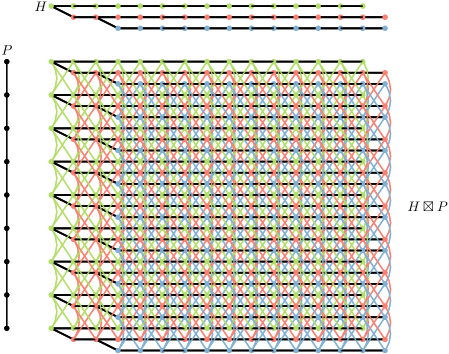
Figure 2: The strong product of a tree $H$ and a path $P$.

4.1 Distance Functions and Metric Spaces

A distance function over a set $S$ is any function $d:S^{2}\to\mathbb{R}\cup\{\infty\}$ that satisfies $d(x,x)=0$ for all $x\in S$; $d(x,y)\geqslant 0$ and $d(x,y)=d(y,x)$ for all distinct $x,y\in S$; and $d(x,z)\leqslant d(x,y)+d(y,z)$ for all distinct $x,y,z\in S$. For any $x\in S$, and any non-empty $Z\subseteq S$, $\leavevmode\color[rgb]{0.76,0.13,0.28}d(x,Z):=\min(\{d(x,y):y\in Z\}\cup\{\infty\})$. A metric space $\mathcal{M}:=(S,d)$ consists of a set $S$ and a distance function $d$ over (some superset of) $S$. $\mathcal{M}$ is finite if $S$ is finite and $\mathcal{M}$ is non-empty if $S$ is non-empty. For $x\in S$ and $r\geqslant 0$, the $r$-ball centered at $x$ is $\leavevmode\color[rgb]{0.76,0.13,0.28}B_{\mathcal{M}}(x,r):=\{y\in S:d(x,y)\leqslant r\}$. The diameter of a non-empty finite metric space $(S,d)$ is $\leavevmode\color[rgb]{0.76,0.13,0.28}\operatorname{diam}_{d}(S):=\max\{d(x,y):x,y\in S\}$, and the minimum-distance of $(S,d)$ is $\leavevmode\color[rgb]{0.76,0.13,0.28}\operatorname{min-dist}_{d}(S):=\min(\{d(x,y):\{x,y\}\in\binom{S}{2}\}\cup\{\infty\})$.

For any graph $G$, $d_{G}$ is a distance function over $V(G)$, so $\leavevmode\color[rgb]{0.76,0.13,0.28}\mathcal{M}_{G}:=(V(G),d_{G})$ is a metric space. Any metric space that can be defined this way is referred to as a graph metric. For any $S\subseteq V(G)$, the diameter and minimum-distance of $S$ in $G$ are defined as $\leavevmode\color[rgb]{0.76,0.13,0.28}\operatorname{diam}_{G}(S):=\operatorname{diam}_{d_{G}}(S)$ and $\leavevmode\color[rgb]{0.76,0.13,0.28}\operatorname{min-dist}_{G}(S):=\operatorname{min-dist}_{d_{G}}(S)$, respectively.

Since we work with strong products it is worth noting that, for any two graphs $A$ and $B$,

$$d_{A\boxtimes B}((x_{1},x_{2}),(y_{1},y_{2}))=\max\{d_{A}(x_{1},y_{1}),d_{B}(x_{2},y_{2})\}\enspace.$$

Define the local density of a non-empty finite metric space $\mathcal{M}=(S,d)$ to be

$$\leavevmode\color[rgb]{0.76,0.13,0.28}\operatorname{ld}(\mathcal{M}):=\max\{(B_{\mathcal{M}}(x,r)-1)/r:x\in S,\,r>0\}.$$

(This maximum exists because $S$ is finite, so there are only $\binom{|S|}{2}$ values of $r$ that need to be considered.) Thus, if $\mathcal{M}$ has local density at most $D$, then $|B_{\mathcal{M}}(x,r)|\leqslant Dr+1$ for each $x\in S$ and $r\geqslant 0$. This definition is consistent with the definition of local density of graphs: A graph $G$ has local density at most $D$ if and only if the metric space $\mathcal{M}_{G}$ has local density at most $D$. Note that, if $(S,d)$ has local density at most $D$ then $(S,d)$ has $\operatorname{diam}_{d}(S)\geqslant(|S|-1)/D$ and $\operatorname{min-dist}(S)\geqslant 1/D$.

A contraction of a metric space $\mathcal{M}=(S,d)$ into a metric space $\mathcal{M^{\prime}}=(S^{\prime},d^{\prime})$ is a function $\phi:S\to S^{\prime}$ that satisfies $d^{\prime}(\phi(x),\phi(y))\leqslant d(x,y)$, for each $x,y\in S$. The distortion of $\phi$ is $\max\{d(x,y)/d^{\prime}(\phi(x),\phi(y)):\{x,y\}\in\binom{S}{2}\}$. When $S\subseteq S^{\prime}$ and $\phi$ is the identity function, we say that $\mathcal{M^{\prime}}$ is a contraction of $\mathcal{M}$. In particular, saying that $(S,d^{\prime})$ is a contraction of $(S,d)$ is equivalent to saying that $d^{\prime}(x,y)\leqslant d(x,y)$ for all $x,y\in S$.

For two points $x,y\in\mathbb{R}^{L}$, let $\leavevmode\color[rgb]{0.76,0.13,0.28}d_{2}(x,y)$ denote the Euclidean distance between $x$ and $y$. A contraction of $(S,d)$ into $(\mathbb{R}^{L},d_{2})$ for some $L\geqslant 1$ is called a Euclidean contraction. For $K\subseteq S$ we abuse notation slightly with the shorthand $\leavevmode\color[rgb]{0.76,0.13,0.28}\phi(K):=\{\phi(x):x\in K\}$. We make use of two easy observations that follow quickly from these definitions:

Observation 28.

Let $\mathcal{M}:=(S,d)$ and $\mathcal{M}^{\prime}:=(S^{\prime},d^{\prime})$ be non-empty finite metric spaces. If $\mathcal{M^{\prime}}$ has local density $D$ and $\mathcal{M}$ has an injective contraction into $\mathcal{M}^{\prime}$ then $\mathcal{M}$ has local density at most $D$.

Proof.

Let $\phi:S\to S^{\prime}$ be an injective contraction of $\mathcal{M}$ into $\mathcal{M}^{\prime}$. For every $x\in S$, every $r>0$, and every $y\in B_{\mathcal{M}}(x,r)$, we have $d^{\prime}(\phi(x),\phi(y))\leqslant d(x,y)\leqslant r$, since $\phi$ is a contraction. Therefore, $B_{\mathcal{M^{\prime}}}(\phi(x),r)\supseteq\phi(B_{\mathcal{M}}(x,r))$. Since $\phi$ is injective, $|B_{\mathcal{M^{\prime}}}(\phi(x),r)|\geqslant|\phi(B_{\mathcal{M}}(x,r))|=|B_{\mathcal{M}}(x,r)|$. Since $\mathcal{M}^{\prime}$ has local density at most $D$, $rD+1\geqslant|B_{\mathcal{M^{\prime}}}(\phi(x),r)|\geqslant|B_{\mathcal{M}}(x,r))|$. ∎

Observation 29.

For any graph $I$ and any subgraph $G$ of $I$, $(V(G),d_{I})$ is a contraction of $(V(G),d_{G})$.

Proof.

From the definitions, it follows that $d_{I}$, restricted to $V(G)$ is a distance function over $V(G)$, so $(V(G),d_{I})$ is a metric space. Since $G$ is a subgraph of $I$, every path in $G$ is also a path in $I$ so, $d_{I}(x,y)\leqslant d_{G}(x,y)$ for each $x,y\in V(G)$. ∎

4.2 Volume-Preserving Contractions

For a set $K$ of $k\leqslant L+1$ points in $\mathbb{R}^{L}$, the Euclidean volume of $K$, denoted by $\leavevmode\color[rgb]{0.76,0.13,0.28}\operatorname{Evol}(K)$, is the $(k-1)$-dimensional volume of the simplex whose vertices are the points in $K$. For example, if $k=3$, then $\operatorname{Evol}(K)$ is the area of the triangle whose vertices are $K$ and that is contained in a plane that contains $K$.

Define the ideal volume of a finite metric space $(K,d)$ to be

$$\leavevmode\color[rgb]{0.76,0.13,0.28}\operatorname{Ivol}_{d}(K):=\max\{\operatorname{Evol}(\phi(K)):\text{$\phi$ is a Euclidean contraction of $(K,d)$}\}.$$

A Euclidean contraction $\phi:S\to\mathbb{R}^{\ell}$ of a finite metric space $(S,d)$ is $(k,\eta)$-volume-preserving if $\operatorname{Evol}(\phi(K))\geqslant\operatorname{Ivol}_{d}(K)/\eta^{k-1}$ for each $k$-element subset $K$ of $S$. This definition is a generalization of distortion: $\phi$ is $(2,\eta)$-volume-preserving if and only if $\phi$ has distortion at most $\eta$.

Feige [32] introduces the following definition and theorem as a bridge between ideal volume and Euclidean volume. The tree volume of a finite metric space $(K,d)$ is defined as $\leavevmode\color[rgb]{0.76,0.13,0.28}\operatorname{Tvol}_{d}(K):=\prod_{xy\in E(T)}d(x,y)$ where $T$ is a minimum spanning tree of the weighted complete graph with vertex set $K$ where the weight of each edge $xy$ is equal to $d(x,y)$. The following lemma makes tree volume a useful intermediate measure when trying to establish that a contraction is volume-preserving.

Lemma 30 (Feige [32, Theorem 3]).

For any finite metric space $(S,d)$ with $|S|=k$,

$$\operatorname{Ivol}_{d}(S)\leqslant\frac{\operatorname{Tvol}_{d}(S)}{(k-1)!}\leqslant 2^{(k-2)/2}\operatorname{Ivol}_{d}(S)\enspace.$$

4.3 Bandwidth from Local Density and Volume-Preserving Contractions

The following lemma, whose proof appears in Appendix A, generalizes Feige [32, Theorem 10] from graph metrics to general metric spaces and establishes a critical connection between local density and tree volume.

Lemma 31 (Generalization of [T]heorem 10).

feige:approximating] For every $n$-element metric space $\mathcal{M}:=(S,d)$ with local density at most $D$ and every positive integer $k$,

$$\sum_{K\in\binom{S}{k}}\frac{1}{\operatorname{Tvol}_{d}(K)}<n(DH_{n}/2)^{k-1}\enspace,$$

where $\leavevmode\color[rgb]{0.76,0.13,0.28}H_{n}:=\sum_{i=1}^{n}1/i\leqslant 1+\ln n$ is the $n$-th harmonic number.

Theorem 33, which appears below and whose proof appears in Appendix B, is a generalization of Theorem 17 from graph metrics to arbitrary metrics. First, we need a definition of bandwidth for metric spaces. Let $(S,d)$ be a non-empty finite metric space and let $x_{1},\ldots,x_{n}$ be a permutation of $S$. Then $\leavevmode\color[rgb]{0.76,0.13,0.28}\operatorname{bw}_{(S,d)}(x_{1},\ldots,x_{n}):=\max\{j-i:d(x_{i},x_{j})\leqslant 1,\,1\leqslant i<j\leqslant n\}$ and $\leavevmode\color[rgb]{0.76,0.13,0.28}\operatorname{bw}(S,d)$ is the minimum of $\operatorname{bw}_{(S,d)}(x_{1},\ldots,x_{n})$ taken over all $n!$ permutations $x_{1},\ldots,x_{n}$ of $S$. Note that this coincides with the definition of the bandwidth of a graph: For any connected graph $G$, $\operatorname{bw}(\mathcal{M}_{G})=\operatorname{bw}(G)$. First we observe that injective contractions can only increase bandwidth:

Observation 32.

For every finite metric space $\mathcal{M}:=(S,d)$ and every (injective) contraction $\mathcal{M}^{\prime}:=(S,d^{\prime})$ of $\mathcal{M}$, $\operatorname{bw}(\mathcal{M})\leqslant\operatorname{bw}(\mathcal{M}^{\prime})$.

Proof.

Let $x_{1},\ldots,x_{n}$ be an ordering of the elements of $S$ such that $b:=\operatorname{bw}(\mathcal{M}^{\prime})=\operatorname{bw}_{\mathcal{M}}(x_{1},\ldots,x_{n})$. Consider any pair of elements $x_{i}x_{j}$ with $d(x_{i},x_{j})\leqslant 1$. Since $\mathcal{M}^{\prime}$ is a contraction of $\mathcal{M}$, $d^{\prime}(x_{i},x_{j})\leqslant 1$. Since $\operatorname{bw}_{\mathcal{M}^{\prime}}(x_{1},\ldots,x_{n})\leqslant b$, $|j-i|\leqslant b$. Thus $\operatorname{bw}(\mathcal{M})\leqslant\operatorname{bw}_{\mathcal{M}}(x_{1},\ldots,x_{n})\leqslant b$. ∎

Theorem 33 (Generalization of Theorem 17).

Let $(S,d)$ be a $n$-element metric space with local density at most $D$ and diameter at most $\Delta$. If $(S,d)$ has a $(k,\eta)$-volume-preserving Euclidean contraction $\phi:S\to\mathbb{R}^{L}$ then

$$\operatorname{bw}(S,d)\in O((nk\log\Delta)^{1/k}\,Dk\eta\log^{3/2}n)\enspace.$$

4.4 Proof of Theorem 7

We are now ready to prove Theorem 7. The entirety of this subsection should be treated as a proof of Theorem 7. Most of the results in this section are written as claims that are not self-contained, since they refer $G$, $H$, $P$, $X$, $d^{*}$, and other objects defined throughout this subsection. From this point on, $\leavevmode\color[rgb]{0.76,0.13,0.28}G$ is an $n$-vertex subgraph of $H\boxtimes P$ where $\leavevmode\color[rgb]{0.76,0.13,0.28}H$ is a $t$-tree (an edge-maximal graph of treewidth $t$) and $\leavevmode\color[rgb]{0.76,0.13,0.28}P$ is a path.

We now outline the structure of our proof. (We use the notation $\mathcal{M}\rightbroom\mathcal{M^{\prime}}$ to denote that $\mathcal{M}^{\prime}$ is a contraction of $\mathcal{M}$.)

1. Use a variant of Lemma 21 to find a set $X\subseteq V(H\boxtimes P)$ of size $O((tn\log n)/D)$ such that the metric space $\mathcal{M}:=(V(G-X),d_{(H\boxtimes P)-X})$ has local density at most $D$. (In the final step of the proof, $D$ is set to $\sqrt{tn}/\log n$.) Since $G-X$ is a subgraph of $(H\boxtimes P)-X$, Observation 29 implies that $\mathcal{M}$ is a contraction of the metric space $\mathcal{M}_{G-X}:=(V(G-X),d_{G-X})$, so $\mathcal{M}_{G-X}\rightbroom\mathcal{M}$.

2. Design a distance function $d^{*}:V((H\boxtimes P)-X)^{2}\to\mathbb{R}$ so that the metric space $\mathcal{M}^{*}:=(V(H\boxtimes P)\setminus X,d^{*})$ is a contraction of $\mathcal{M}$ with the property that the induced metric space $(V(G-X),d^{*})$ has local density at most $D$.

   Graphically, $\mathcal{M}_{G-X}\rightbroom\mathcal{M}\rightbroom\mathcal{M}^{*}$.

3. Prove that $\mathcal{M}^{*}$ has a $(k,O(\sqrt{\log n}))$-volume-preserving Euclidean contraction, for $k={\lceil\log n\rceil}$. The preceding two steps are done in such a way that this part of the proof is able to closely follow the proof of Theorem 16 by Rao [45].

4. By Theorem 33, $\operatorname{bw}(\mathcal{M}^{*})\in O(D\log^{3}n)=O(\sqrt{tn}\log^{2}n)$. Since $\mathcal{M}^{*}$ is a contraction of $\mathcal{M}_{G-X}$, Observation 32 implies that $\operatorname{bw}(G-X)=\operatorname{bw}(\mathcal{M}_{G-X})\leqslant\operatorname{bw}(\mathcal{M}^{*})\in O(\sqrt{tn}\log^{2}n)$.

The delicate part of the proof is the design of the distance function $d^{*}$ that contracts $d_{(H\boxtimes P)-X}$ but still ensures that the local density of $(V(G-X),d^{*})$ is at most $D$. If $d^{*}$ contracts too much, then $(V(G-X),d^{*})$ will not have local density $O(D)$. If $d^{*}$ contracts too little, then it will be difficult to get a $(k,O(\sqrt{\log n}))$-volume-preserving Euclidean embedding of $\mathcal{M}^{*}$. To make all of this work, the distance function $d^{*}$ makes use of the structure of the sparsifying set $X$.

4.4.1 A Structured Sparsifier

In this section, we construct a sparsifying set $X$ like that used in Lemma 18. The main difference is that we do not use a BFS layering of $G$ when applying Lemma 21. Instead, we use the layering of $G$ that comes from $H\boxtimes P$. Although this is really the only difference, we repeat most of the steps in the proof of Lemma 21 in order to establish notations and precisely define the structure of $X$, which will be useful in the design of the distance function $d^{*}$. In particular, later sections rely on the structure of the individual subsets $X_{i,j}$ whose union is $X$.

Let $N:=2^{{\lceil\log n\rceil}}$ and let $P:=\leavevmode\color[rgb]{0.76,0.13,0.28}y_{-N+1},y_{-N+2},\ldots,y_{2N}$ be a path. Without loss of generality we assume all vertices of $G$ are contained in $V(H)\times\{y_{1},\ldots,y_{N}\}$. For each $i\in\{0,\ldots,\log N\}$ and each $j\in\{-1,0,\ldots,N/2^{i}\}$, let $P_{i,j}:=y_{j2^{i}+1},\ldots,y_{(j+1)2^{i}}$ be a subpath of $P$ with $2^{i}$ vertices. For each $i\in\{0,\ldots,\log N\}$ and each $j\in\{0,\ldots,N/2^{i}-1\}$, let $P^{+}_{i,j}:=P[V(P_{i,j-1})\cup V(P_{i,j})\cup V(P_{i,j+1})]$ be the concatenation of $P_{i,j-1}$, $P_{i,j}$, and $P_{i,j+1}$. Define $Q_{i,j}\coloneqq H\boxtimes P_{i,j}$ and $Q^{+}_{i,j}\coloneqq H\boxtimes P^{+}_{i,j}$. In words, $Q_{i,0},\ldots,Q_{i,N/2^{i}-1}$ partitions the part of $H\boxtimes P$ that contains $G$ into vertex-disjoint strips of height $2^{i}$. Each subgraph $Q^{+}_{i,j}$ is a strip of height $3\cdot 2^{i}$ that contains $Q_{i,j}$ in its middle third.

To construct our sparsifying set $X$, we first construct vertex subsets $Y_{i,j}$ of $H$ for each $i\in\{0,1,\ldots,\log N\}$ and $j\in\{0,\ldots,N/2^{i}-1\}$. Define the weight function $\xi_{i,j}:V(H)\to\mathbb{N}$ where $\xi_{i,j}(x):=|(\{x\}\times V(P^{+}_{i,j}))\cap V(G)|$. Observe that $\xi_{i,j}(H):=\sum_{x\in V(H)}\xi_{i,j}(x)=|V(Q^{+}_{i,j})\cap V(G)|$. Let $D\geqslant 2$ be a real number. By Lemma 20 with $c:=\lceil\xi_{i,j}(H)/(2^{i-1}D)\rceil$, there exists $Y_{i,j}\subseteq V(H)$ of size at most $(t+1)\xi_{i,j}(H)/(2^{i-1}D)$, such that each component $C$ of $H-Y_{i,j}$ has total weight $\xi_{i,j}(C)\leqslant 2^{i-1}D$. For each $i\in\{0,1,\ldots,\log N\}$ and $j\in\{0,\ldots,N/2^{i}-1\}$, let $\leavevmode\color[rgb]{0.76,0.13,0.28}X_{i,j}:=Y_{i,j}\times V(P^{+}_{i,j})$. We think of $X_{i,j}$ as a vertical separator that splits the strip $Q^{+}_{i,j}$ into parts using vertex cuts that run from the top to the bottom of $Q^{+}_{i,j}$.

Claim 34.

For each $i\in\{0,,\ldots,\log N\}$ and $j\in\{0,\ldots,N/2^{i}-1\}$, each component of $Q^{+}_{i,j}-X_{i,j}$ has at most $2^{i-1}D$ vertices.

Proof.

The number of vertices of $G$ in a component $C$ of $Q^{+}_{i,j}-X_{i,j}$ is equal to the total weight $\zeta_{i,j}(C_{H})$ of the corresponding component $C_{H}$ of $H-Y_{i,j}$. Therefore, each component of $Q^{+}_{i,j}-X_{i,j}$ contains at most $2^{i-1}D$ vertices of $G$. ∎

Let

$$\leavevmode\color[rgb]{0.76,0.13,0.28}X:=\bigcup_{i=0}^{\log N}\bigcup_{j=0}^{N/2^{i}-1}X_{i,j}\enspace.$$

Claim 35.

$|X|\leqslant 18(t+1)n(1+\log N)/D$.

Proof.

Observe that $\sum_{j=0}^{N/2^{i}-1}\xi_{i,j}(H)\leqslant\sum_{j=0}^{N/2^{i}-1}3|V(G_{i,j})|\leqslant 3n$, since, each vertex $v$ of $G$ can only appear in $Q^{+}_{i,j-1},Q^{+}_{i,j}$, and $Q^{+}_{i,j+1}$ where $j$ is the unique index such that $v\in V(Q_{i,j})$. By definition, $|X_{i,j}|=3\cdot 2^{i}\cdot|Y_{i,j}|\leqslant 6(t+1)\xi_{i,j}(H)/D$. Therefore, $\sum_{j=0}^{N/2^{i}-1}|X_{i,j}|\leqslant 18(t+1)n/D$. Summing over $i\in\{0,\ldots,\log N\}$ completes the proof. ∎

4.4.2 The Distance Function $d^{*}$

In order to construct a volume-preserving Euclidean contraction $\phi$ for a distance function $d$ we must ensure (at least) that $d_{2}(\phi(v),\phi(w))$ is large whenever $d(v,w)$ is large. This is relatively easy to do for the distance function $d_{H\boxtimes P}$ using (simplifications of) the techniques used by Rao [45] for planar graphs. This is more difficult for $d_{(H\boxtimes P)-X}$ because distances are larger, which only makes the problem harder. Some of these distances are necessarily large; the obstacles in $X$ are needed to ensure that $(V(G),d_{(H\boxtimes P)-X})$ has local density at most $D$. The purpose of a single set $X_{i,j}$ is to increase distances between some pairs of vertices in $Q^{+}_{i,j}$ so that they are at least $2^{i}$. However, the obstacles in $X$ sometimes interact, by chance, to make distances excessively large. Figure 3 shows that, even when $H=P$, obstacles in $X_{i,j+1}$ and in $X_{i,j-1}$ can interact in such a way that $d_{(H\boxtimes P)-X}(v,w)$ can become $r2^{i}$ for arbitrarily large $r$. This large distance is not needed to ensure the local density bound and it makes it difficult to construct a volume-preserving Euclidean contraction of $(V(G),d_{(H\boxtimes P)-X})$. The purpose of the intermediate distance function $d^{*}$ is to reduce these unnecessarily large distances so that $d^{*}(v,w)$ is defined only by the “worst” obstacle in $X$ that separates $v$ and $w$.

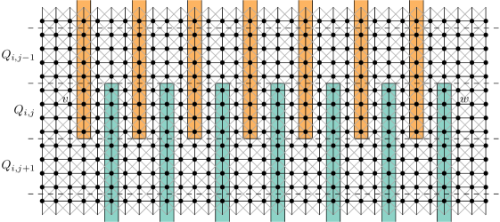
Figure 3: Obstacles not in $X_{i,j}$ can interact to create excessively large distances between vertices in $Q_{i,j}$.

For any subgraph $A^{\prime}$ of a graph $A$, we use the shorthand $\overline{A}^{\prime}:=V(A)\setminus V(A^{\prime})$. (When we use this notation, the graph $A$ will be clear from context.) For any vertex $u$ of $H\boxtimes P$, let $u_{P}$ denote the second coordinate of $u$ (the projection of $u$ onto $P$). Let $u$ and $v$ be two vertices of $(H\boxtimes P)-X$. If $u$ and $v$ are both vertices of $Q^{+}_{i,j}$ but are in different components of $Q^{+}_{i,j}-X_{i,j}$, then define

$$\leavevmode\color[rgb]{0.76,0.13,0.28}d_{i,j}(u,v):=\min\{d_{P}(u_{P},x)+d_{P}(x,v_{P}):x\in\overline{P}^{+}_{i,j}\}\enspace.$$

Otherwise (if one of $u$ or $v$ is not in $Q^{+}_{i,j}$ or $u$ and $v$ are in the same component of $Q^{+}_{i,j}-X_{i,j}$), define $\leavevmode\color[rgb]{0.76,0.13,0.28}d_{i,j}(u,v):=0$. When $d_{i,j}(u,v)>0$, it is helpful to think of $d_{i,j}(u,v)$ as the length of the shortest walk in $P$ that begins at $u_{P}$, leaves $P^{+}_{i,j}$ and returns to $v_{P}$. Now define our distance function

$$\leavevmode\color[rgb]{0.76,0.13,0.28}d^{*}(u,v):=\max\left(\{d_{H\boxtimes P}(u,v)\}\cup\left\{d_{i,j}(u,v):(i,j)\in\{0,\ldots,\log N\}\times\{1,\ldots,N/2^{i}-1\}\right\}\right)$$

Intuitively, $d^{*}(u,v)$ captures the fact that any path from $u$ to $v$ in $(H\boxtimes P)-X$ must navigate around each obstacle $X_{i,j}$ that separates $u$ and $v$ in the graph $Q^{+}_{i,j}$. At the very least, this requires a path from $u$ to some vertex $x$ outside of $Q^{+}_{i,j}$ followed by a path from $x$ to $v$. The length of this path is at least the length of the shortest walk in $P$ that begins at $u_{P}$, contains $x_{P}$ and ends at $w_{P}$.

Claim 36.

The function $d^{*}:V((H\boxtimes P)-X)\to\mathbb{N}\cup\{\infty\}$ is a distance function for $V((H\boxtimes P)-X)$.

Proof.

It is straightforward to verify that $d^{*}(u,u)=0$ for all $u\in V((H\boxtimes P)\setminus X)$ and that $d^{*}(u,v)=d(v,u)\geqslant 0$ for all $u,v\in V((H\boxtimes P)-X)$. It only remains to verify that $d^{*}$ satisfies the triangle inequality. We must show that, for distinct $u,v,w\in V((H\boxtimes P)-X)$, $d^{*}(u,w)\leqslant d^{*}(u,v)+d^{*}(v,w)$.

If $d^{*}(u,w)=0$ then $d^{*}(u,v)+d^{*}(v,w)\geqslant 0=d^{*}(u,w)$ and we are done. If $d^{*}(u,w)=d_{H\boxtimes P}(u,w)$ then $d^{*}(u,v)+d^{*}(v,w)\geqslant d_{H\boxtimes P}(u,v)+d_{H\boxtimes P}(v,w)\geqslant d_{H\boxtimes P}(u,w)$ and we are also done. Otherwise, $d^{*}(u,w)=d_{i,j}(u,w)>0$ for some $i,j$. Then $u$ and $w$ are vertices of $Q^{+}_{i,j}$ that are in different components of $Q^{+}_{i,j}-X_{i,j}$. There are two cases to consider, depending on the location of $v$:

1. If $v\not\in V(Q^{+}_{i,j})$ then $d^{*}(u,v)+d^{*}(v,w)\geqslant d_{H\boxtimes P}(u,v)+d_{H\boxtimes P}(v,w)\geqslant d_{P}(u_{P},v_{P})+d_{P}(v_{P},w_{P})\geqslant d_{i,j}(u,w)=d^{*}(u,w)$.

2. If $v\in V(Q^{+}_{i,j})$ then, since $u$ and $w$ are in different components $C_{u}$ and $C_{w}$ of $Q^{+}_{i,j}-X_{i,j}$, at least one of $C_{u}$ or $C_{w}$ does not contain $v$. Without loss of generality, suppose $C_{w}$ does not contain $v$. Then $d^{*}(u,v)+d^{*}(v,w)\geqslant d_{H\boxtimes P}(u,v)+d_{i,j}(v,w)\geqslant d_{P}(u_{P},v_{P})+d_{i,j}(v,w)$. Now, $d_{P}(u_{P},v_{P})$ is the length of a path in $P$ from $u_{P}$ to $v_{P}$ and $d_{i,j}(v,w)$ is the length of a (shortest) walk in $P$ that begins at $v_{P}$, leaves $P^{+}_{i,j}$ and then returns to $w_{P}$. Thus, $d_{P}(u_{P},v_{P})+d_{i,j}(v,w)$ is the length of a walk in $P$ that begins at $u_{P}$, leaves $P^{+}_{i,j}$ and then returns to $w_{P}$. On the other hand, $d_{i,j}(u,w)$ is the length of a shortest walk in $P$ that begins at $u_{P}$, leaves $P^{+}_{i,j}$ and returns to $w_{P}$, so $d_{i,j}(u,w)\leqslant d_{P}(u_{P},v_{P})+d_{i,j}(v,w)$. Therefore, $d^{*}(u,v)+d^{*}(v,w)\geqslant d_{P}(u_{P},v_{P})+d_{i,j}(v,w)\geqslant d_{i,j}(u,w)=d^{*}(u,w)$. ∎

Claim 37.

The metric space $\mathcal{M}^{*}:=(V(G-X),d^{*})$ has local density at most $D$.

Proof.

We must show that, for any $v\in V(G)$ and any $r>0$, $|B_{\mathcal{M}^{*}}(v,r)|\leqslant Dr+1$. If $r\geqslant n/D$ then this is trivial, so assume that $r<n/D$. Consider some vertex $w\in B_{\mathcal{M}^{*}}(v,r)$. Let $i:=\lceil\log r\rceil$ and let $j$ be such that $v$ is a vertex of $Q_{i,j}$. Since $w\in B_{\mathcal{M}^{*}}(v,r)$, $d_{H\boxtimes P}(v,w)\leqslant r\leqslant 2^{i}$. Therefore $d_{P}(v_{P},w_{P})\leqslant d_{H\boxtimes P}(v,w)\leqslant 2^{i}$. Therefore $w$ is contained in $Q^{+}_{i,j}$. Since $d^{*}(v,w)\leqslant r$, $d_{i,j}(v,w)\leqslant r$. This implies that $v$ and $w$ are in the same component of $Q^{+}_{i,j}-X_{i,j}$ since, otherwise, $d_{i,j}(v,w)\geqslant d_{P}(u_{P},\overline{P}^{+}_{i,j})+d_{P}(\overline{P}^{+}_{i,j},w_{P})\geqslant 2^{i}+1$. Therefore, $B_{\mathcal{M}^{*}}(v,r)$ is contained in the component $C$ of $Q^{+}_{i,j}-X_{i,j}$ that contains $v$. By 34, $|V(C)|\leqslant 2^{i-1}D<rD$. Therefore, $|B_{\mathcal{M}^{*}}(v,r)|\leqslant|V(C)|<rD$. ∎

Claim 38.

The metric space $(V(H\boxtimes P)\setminus X,d^{*})$ is a contraction of $\mathcal{M}_{(H\boxtimes P)-X}=(V((H\boxtimes P)-X),d_{(H\boxtimes P)-X})$.

Proof.

Let $u$ and $v$ be distinct vertices of $(H\boxtimes P)-X$. If $d^{*}(u,v)=d_{H\boxtimes P}(u,v)$ then, $d^{*}(u,v)=d_{H\boxtimes P}(u,v)\leqslant d_{(H\boxtimes P)-X}(u,v)$. If $d^{*}(u,v)=d_{i,j}(u,v)$ for some $i$ and $j$ then any path from $u$ to $v$ in $(H\boxtimes P)-X$ must contain some vertex $x$ not in $Q^{+}_{i,j}$ since $u$ and $v$ are in different components of $Q^{+}_{i,j}-X$. The shortest such path has length at least $d_{H\boxtimes P}(u,x)+d_{H\boxtimes P}(x,v)\geqslant d_{P}(u_{P},x_{P})+d_{P}(x_{P},v_{P})\geqslant d_{i,j}(u,v)=d^{*}(u,v)$. ∎

The preceding claims are summarized in the following corollary:

Corollary 39.

The metric space $(V((H\boxtimes P)-X),d^{*})$ is a contraction of $(V((H\boxtimes P)-X),d_{(H\boxtimes P)-X})$ and the metric space $(V(G-X),d^{*})$ has local density at most $D$.

4.4.3 Volume-Preserving Contraction of $\mathcal{M}^{*}$

In this subsection we prove the following result:

Claim 40.

For every integer $k\in\{2,\ldots,n\}$, the metric space $\mathcal{M}^{*}:=(V(G-X),d^{*})$ has a $(k,O(\sqrt{\log n}))$-volume-preserving Euclidean contraction.

Decomposing $H\boxtimes P$.

Let $\Delta\geqslant 4$ be a power of $2$. We now show how to randomly decompose $H\boxtimes P$ into subgraphs $\{(H\boxtimes P)^{\Delta}_{a,b}:(a,b)\in\mathbb{Z}^{2}\}$. The only randomness in this decomposition comes from choosing two independent uniformly random integers $r_{H}$ and $r_{P}$ in $\{0,\ldots,\Delta-1\}$. See Figure 4, for an example.

Figure 4: The result of decomposing the graph $H\boxtimes P$ in Figure 2 with $\Delta=4$, $r_{H}=2$, and $r_{P}=3$.

Let $\{L_{s}:s\in\mathbb{Z}\}$ be a BFS layering of $H$. For each integer $a$, let $H^{\Delta}_{a}:=H[\bigcup_{s=r_{H}+a\Delta}^{r_{H}+(a+1)\Delta-1}L_{s}]$ so that $\{H^{\Delta}_{a}:a\in\mathbb{Z}\}$ is a pairwise vertex-disjoint collection of induced subgraphs that covers $V(H)$ and each $H^{\Delta}_{a}$ is a subgraph of $H$ induced by $\Delta$ consecutive BFS layers. For each integer $b$, let $P^{\Delta}_{b}:=P[\{y_{r_{P}+b\Delta},\ldots,y_{r_{P}+(b+1)\Delta-1}]$ so that $\{P^{\Delta}_{b}:b\in\mathbb{Z}\}$ is a collection of vertex disjoint paths, each having $\Delta$ vertices, that cover $P$. For each $(a,b)\in\mathbb{Z}^{2}$, let $(H\boxtimes P)^{\Delta}_{a,b}:=H^{\Delta}_{a}\boxtimes P^{\Delta}_{b}$.

Claim 41.

For each $(a,b)\in\mathbb{Z}^{2}$, each component $C$ of $(H\boxtimes P)^{\Delta}_{a,b}$ has $\operatorname{diam}_{H\boxtimes P}(C)\leqslant 2\Delta+1$.

Proof.

Let $v:=(v_{1},v_{2})$ and $w:=(w_{1},w_{2})$ be two vertices of $(H\boxtimes P)^{\Delta}_{a,b}$. Our task is to show that $d_{H\boxtimes P}(v,w)\leqslant 2\Delta+1$. Recall that $d_{H\boxtimes P}(v,w)=\max\{d_{H}(v_{1},w_{1}),d_{P}(v_{2},w_{2})\}$. Since $P^{\Delta}_{b}$ is a subpath of $P$ with $\Delta$ vertices, $d_{P}(v_{2},w_{2})=d_{P^{\Delta}_{b}}(v_{2},w_{2})\leqslant\Delta-1$, so we need only upper bound $d_{H}(v_{1},w_{1})$.

To do this, we make use of the following property of BFS layerings of $t$-trees [40, 23]: For every integer $s$, for each component $C$ of $H[L_{s+1}]$, the set $N_{C}$ of vertices in $L_{s}$ that are adjacent to at least one vertex in $C$ form a clique in $H$. Since $v_{1}$ and $w_{1}$ are in the same component $A$ of $H^{\Delta}_{a}$, this implies that $C:=A[L_{r_{H}+a\Delta}]$ is connected. This implies that the set $N_{C}$ of vertices in $L_{r_{H}+a\Delta-1}$ adjacent to vertices in $C$ form a clique. Then $H^{\Delta}_{a}$ contains a path of length at most $\Delta$ from $v_{1}$ to a vertex $v_{1}^{\prime}$ in $N_{C}$. Likewise, $H^{\Delta}_{a}$ contains a path of length at most $\Delta$ from $w$ to a vertex $w^{\prime}$ in $N_{C}$. Since $N_{C}$ is clique $v^{\prime}=w^{\prime}$ or $v^{\prime}$ and $w^{\prime}$ are adjacent. In the former case, there is a path in $H$ from $v$ to $w$ of length at most $2\Delta$. In the latter case there is a path from $v$ to $w$ of length at most $2\Delta+1$. ∎

Claim 42.

Fix some vertex $v$ of $H\boxtimes P$ independently of $r_{H}$ and $r_{P}$ and let $(a,b)$ be such that $v$ is a vertex of $(H\boxtimes P)^{\Delta}_{a,b}$. Then, with probability at least $1/4$,

$$d_{H\boxtimes P}(v,\overline{(H\boxtimes P)}^{\Delta}_{a,b})\geqslant\Delta/4.$$

Proof.

Let $v:=(v_{1},v_{2})$. Let $\mathcal{E}$ be the event $d_{H\boxtimes P}(v,V(H\boxtimes P)\setminus V((H\boxtimes P)_{a,b}^{\Delta}))\geqslant\Delta/4$, let $\mathcal{E}_{H}$ be the event $d_{H}(v_{1},\overline{H}^{\Delta}_{a})\geqslant\Delta/4$ and let $\mathcal{E}_{P}$ be the event $d_{P}(v_{2},\overline{P}^{\Delta}_{b})\geqslant\Delta/4$. Then $\mathcal{E}=\mathcal{E}_{H}\cap\mathcal{E}_{P}$.

Recall that our partition is defined in terms of a BFS layering $\{L_{i}:i\in\mathbb{Z}\}$ of $H$ and a random offset $r_{H}\in\{0,\ldots,\Delta-1\}$. The complementary event $\overline{\mathcal{E}}_{H}$ occurs if and only if $(i\bmod\Delta)-r_{H}\in\{-\Delta/4-1,\ldots,\Delta/4-1\}$. The number of such $r_{H}$ is $\Delta/2-1$, so $\Pr(\overline{\mathcal{E}}_{H})=(\Delta/2-1)/\Delta<1/2$ and $\Pr(\mathcal{E}_{H})>1/2$. Similarly $\overline{\mathcal{E}}_{P}$ occurs if and only if $v_{2}=y_{j}$ and $|(j\bmod\Delta)-r_{P}|\in\{-\Delta/4-1,\ldots,\Delta/4-1\}$ which also occurs with probability less than $1/2$, so $\Pr(\mathcal{E}_{P})>1/2$.

The events $\mathcal{E}_{H}$ and $\mathcal{E}_{P}$ are independent since the occurrence of $\mathcal{E}_{H}$ is determined entirely by the choice of $r_{H}$ and the occurence of $\mathcal{E}_{P}$ is determined entirely by the choice of $r_{P}$. Therefore $\Pr(\mathcal{E})=\Pr(\mathcal{E}_{H})\cdot\Pr(\mathcal{E}_{P})>1/4$. ∎

The Coordinate Function $\varphi_{I}$.

Let $I$ be the union of the vertex-disjoint graphs $(H\boxtimes P)^{\Delta}_{a,b}$ over all integer $a$ and $b$. Thus, $I$ is a random subgraph of $H\boxtimes P$ whose value depends only on the random choices $r_{H}$ and $r_{P}$. For each component $C$ of $I$, let $X_{C}:=\cup\{X_{i,j}:C\subseteq Q^{+}_{i,j},\,i\in\{0,\ldots,\log N\},j\in\{0,\ldots,N/2^{i}-1\}\}$. In words, $X_{C}$ contains only the vertical cuts used to construct $X$ that cut $C$ from top to bottom. Let $J$ be the subgraph of $I$ obtained by removing, for each component $C$ of $I$, the vertices in $X_{C}\cap V(C)$.

Claim 43.

Each component $C^{\prime}$ of $J$ has $\operatorname{diam}_{d^{*}}(C^{\prime})\leqslant 5\Delta$.

Proof.

Let $C^{\prime}$ be a component of $J$, let $C$ be the component of $I$ that contains $C^{\prime}$, and let $v$ and $w$ be two vertices of $C^{\prime}$. Our task is to show that $d^{*}(v,w)\leqslant 5\Delta$. By 41, $d_{H\boxtimes P}(v,w)\leqslant 2\Delta+1<5\Delta$, so we may assume that $d^{*}(v,w)\neq d_{H\boxtimes P}(v,w)$. Therefore $d^{*}(v,w)=d_{i,j}(v,w)$ for some $i$ and $j$ such that $v$ and $w$ are in different components of $Q^{+}_{i,j}-X_{i,j}$. Since $v$ and $w$ are in the same component $C$ of $I$, the component $C$ is not contained in $Q^{+}_{i,j}$. (Otherwise, $X_{i,j}$ would be in $X_{C}$ and $v$ and $w$ would be in different components of $J$.) Therefore $C$ contains a vertex $x$ that is not in $Q^{+}_{i,j}$. By 41, $d_{H\boxtimes P}(x,v)\leqslant 2\Delta+1$ and $d_{H\boxtimes P}(x,w)\leqslant 2\Delta+1$. Therefore $d^{*}(v,w)=d_{i,j}(v,w)\leqslant d_{P}(v_{P},x_{P})+d_{P}(x_{P},w_{P})\leqslant d_{H\boxtimes P}(v,x)+d_{H\boxtimes P}(x,w)\leqslant 4\Delta+2\leqslant 5\Delta$. ∎

For each component $C^{\prime}$ of $J$, choose a uniformly random $\alpha_{C^{\prime}}$ in $[0,1]$, with all choices made independently. For each component $C$ of $I$, each component of $C^{\prime}$ of $J$ that is contained in $C$, and each $v\in V(C^{\prime})$, let

$$\varphi_{I}(v):=(1+\alpha_{C^{\prime}})\,d_{H\boxtimes P}(v,\overline{C})\enspace.$$

Observation 44.

Fix $I:=I(H,P,\Delta,r_{H},r_{P})$ and $J:=J(H,P,G)$. For each $v\in V(J)$, $\varphi_{I}(v)$ is uniformly distributed in the real interval $[d_{H\boxtimes P}(v,\overline{C}),\;2d_{H\boxtimes P}(v,\overline{C})]$.

Claim 45.

For every two vertices $v,w\in V(H\boxtimes P)\setminus X$,

$$|\varphi_{I}(v)-\varphi_{I}(w)|\leqslant 2\,d^{*}(v,w)\enspace.$$

Proof.

If $v=w$ then $|\varphi_{I}(v)-\varphi_{I}(w)|=0=2d^{*}(v,w)$, so we assume $v\neq w$. In particular $d^{*}(v,w)\geqslant d_{H\boxtimes P}(v,w)\geqslant 1$. There are three cases to consider, depending on the placement of $v$ and $w$ with respect to the components of $I$ and $J$.

1. If $v$ and $w$ are in different components $C_{v}$ and $C_{w}$ of $I$ then, for some $\alpha_{v},\alpha_{w}\in[0,1]$,

   $$|\varphi_{I}(v)-\varphi_{I}(w)| =|(1+\alpha_{v})d_{H\boxtimes P}(v,\overline{C}_{v})-(1+\alpha_{w})d_{H\boxtimes P}(w,\overline{C}_{w})|$$

   $$<2\max\{d_{H\boxtimes P}(v,\overline{C}_{v}),d_{H\boxtimes P}(w,\overline{C}_{w})\}-\min\{d_{H\boxtimes P}(v,\overline{C}_{v}),d_{H\boxtimes P}(w,\overline{C}_{w})\}$$

   $$\leqslant 2\left(d_{H\boxtimes P}(v,\overline{C}_{v})+d_{H\boxtimes P}(w,\overline{C}_{w})\right)-3$$

   $$\leqslant 2d_{H\boxtimes P}(v,w)-1\leqslant 2d^{*}(v,w)\enspace,$$

   where the penultimate inequality follows from the fact that every path in $H\boxtimes P$ from $v$ to $w$ contains a minimal subpath that begins at $v$ and ends in $\overline{C}_{v}$ and a minimal subpath begins in $\overline{C}_{w}$ and ends at $w$. These two subpaths have at most one edge in common, so $d_{H\boxtimes P}(v,\overline{C}_{v})+d_{H\boxtimes P}(w,\overline{C}_{w})\leqslant d_{H\boxtimes P}(v,w)+1$. We now assume that $v$ and $w$ are in the same component, $C$, of $I$.

2. If $v$ and $w$ are in the same component $C^{\prime}$ of $J$, then $v$ and $w$ are in the same component $C$ of $I$. Then

   $$|\varphi_{I}(v)-\varphi_{I}(w)| =(1+\alpha_{C^{\prime}})|d_{H\boxtimes P}(v,\overline{C})-d_{H\boxtimes P}(w,\overline{C})|$$

   $$\leqslant 2|d_{H\boxtimes P}(v,\overline{C})-d_{H\boxtimes P}(w,\overline{C})|$$

   $$\leqslant 2d_{H\boxtimes P}(v,w)\leqslant 2d^{*}(v,w)\enspace,$$

   where the penultimate inequality is obtained by rewriting the triangle inequalities $d_{H\boxtimes P}(v,\overline{C})\leqslant d_{H\boxtimes P}(v,w)+d_{H\boxtimes P}(w,\overline{C})$ and $d_{H\boxtimes P}(w,\overline{C})\leqslant d_{H\boxtimes P}(w,v)+d_{H\boxtimes P}(v,\overline{C})$.

3. It remains to consider the case where $v$ and $w$ are in the same component $C$ of $I$ but in different components $C^{\prime}_{v}$ and $C^{\prime}_{w}$ of $J$. This happens because there exists some $i$ and $j$ such that $C$ is contained in $Q^{+}_{i,j}$ but $v$ and $w$ are in different components of $Q^{+}_{i,j}-X_{i,j}$. In this case, $d^{*}(v,w)\geqslant d_{i,j}(v,w)=d_{P}(v_{P},x)+d_{P}(x,w_{P})$ for some $x\in\overline{P}^{+}_{i,j}$. Since $C$ is contained in $Q^{+}_{i,j}$, $d_{H\boxtimes P}(v,\overline{C})\leqslant d_{P}(v_{P},x)$ and $d_{H\boxtimes P}(\overline{C},w)\leqslant d_{P}(x,w_{P})$. Therefore $d^{*}(v,w)\geqslant d_{H\boxtimes P}(v,\overline{C})+d_{H\boxtimes P}(w,\overline{C})$. Therefore

   $$|\varphi_{I}(v)-\varphi_{I}(w)| =|(1+\alpha_{C^{\prime}_{v}})d_{H\boxtimes P}(v,\overline{C})-(1+\alpha_{C^{\prime}_{w}})d_{H\boxtimes P}(w,\overline{C})|$$

   $$\leqslant 2\max\{d_{H\boxtimes P}(v,\overline{C}),d_{H\boxtimes P}(\overline{C},w)\}$$

   $$\leqslant 2\left(d_{H\boxtimes P}(v,\overline{C})+d_{H\boxtimes P}(\overline{C},w)\right)$$

   $$\leqslant 2\,d^{*}(v,w)\enspace.\qed$$

The Euclidean Embedding $\phi$.

Let $a>0$ be a constant whose value will be lower-bounded later. We now define a random function $\phi:V((H\boxtimes P)-X)\to\mathbb{R}^{L}$ where $L:=\lfloor 1+\log n\rfloor\cdot\lceil ak\ln n\rceil$. For each $i\in\{0,\ldots,\log N-1\}$ and each $j\in\{1,\ldots,\lceil ak\ln n\rceil\}$, let $I_{i,j}:=I(H,P,2^{i},r_{H,i,j},r_{P,i,j})$ be an instance of the random subgraph $I$ defined in the previous section with parameter $\Delta=2^{i}$ and where random offsets $r_{H,i,j},r_{P,i,j}\in\{0,\ldots,\Delta-1\}$ are chosen independently for each instance. From each $I_{i,j}$ and the sets $\{X_{i^{\prime},j^{\prime}}:i^{\prime}\in\{0,\ldots,\log N-1\},\,j^{\prime}\in\{1,\ldots,N/2^{i}-1\}$, we define the subgraph $J_{i,j}$ of $I_{i,j}$ as in the previous section. This defines a uniformly random $\alpha_{C^{\prime}}$ for each component $C^{\prime}$ of $J_{i,j}$, with all random choices made independently. This defines, for each $v\in V(J_{i,j})$, the value $\varphi_{I_{i,j}}(v)$ and we let $\leavevmode\color[rgb]{0.76,0.13,0.28}\phi_{i,j}(v):=\varphi_{I_{i,j}}(v)$.

Finally, define the Euclidean embedding $\phi:V((H\boxtimes P)-X)\to\mathbb{R}^{L}$ as

$$\phi(x):=\left(\phi_{i,j}(x):(i,j)\in\{0,\ldots,\lfloor\log n\rfloor\}\times\{1,\ldots,\lceil ak\ln n\rceil\}\right)\enspace.$$

The following lemma says that $\phi/2\sqrt{L}$ is a Euclidean contraction of $(V(H\boxtimes P)\setminus X,d^{*})$. In a final step, we divide each coordinate of $\phi$ by $2\sqrt{L}$ to obtain a Euclidean contraction. Until then, it is more convenient to work directly with $\phi$.

Claim 46.

For each $v,w\in V((H\boxtimes P)-X)$,

$$d_{2}(\phi(v),\phi(w))\leqslant 2\sqrt{L}\cdot d^{*}(v,w).$$

Proof.

By 45, $|\phi_{i,j}(v)-\phi_{i,j}(w)|\leqslant 2d^{*}(v,w)$ for each $(i,j)\in\{0,\ldots,\log N\}\times\{1,\ldots,\lceil ak\ln n\rceil\}$. Therefore,

$$d_{2}(\phi(v),\phi(w))=\left(\sum_{i,j}(\phi_{i,j}(v)-\phi_{i,j}(w))^{2}\right)^{1/2}\leqslant\left(L(2d^{*}(v,w))^{2}\right)^{1/2}=2\sqrt{L}\cdot d^{*}(v,w)\enspace.\qed$$

The remaining analysis in this section closely follows Rao [45], which in turn closely follows Feige [32]. The main difference is that we work with $d^{*}$ rather than $d_{G}$. We proceed slowly and carefully since our setting is significantly different, and we expect that many readers will not be familiar with some methods introduced by Feige [32] that are only sketched by Rao [45]. We make use of the following simple Chernoff Bound: For a $\operatorname{binomial}(n,p)$ random variable $B$, $\Pr(B\leqslant np/2)\leqslant\exp(-np/8)$.

Let $\Gamma_{k}:=\{(\lambda_{1},\ldots,\lambda_{k})\in\mathbb{R}^{k}:\sum_{j=1}^{k}\lambda_{j}=1\}$; that is, $\Gamma_{k}$ is the set of coefficients that can be used to obtain an affine combination of $k$ points. In the following lemma, which is the crux of the proofs in [45, 32] it is critical that the function $\lambda$ chooses an affine combination $\lambda_{1},\ldots,\lambda_{p-1}$ by only considering $\phi(v_{1}),\ldots,\phi(v_{p-1})$. Thus any dependence between $\lambda_{1},\ldots,\lambda_{p-1}$ and $\phi(v_{p})$ is limited to the random choices made during the construction of $\phi$ that contribute to $\phi(v_{1}),\ldots,\phi(v_{p-1})$.

Claim 47.

Fix some function $\lambda:(\mathbb{R}^{L})^{p-1}\to\Gamma_{p-1}$. Let $v_{1},\ldots,v_{p}$ be distinct vertices of $(H\boxtimes P)-X$ and let $h:=d^{*}(v_{p},\{v_{1},\ldots,v_{p-1}\})$. Let $(\lambda_{1},\ldots,\lambda_{p-1}):=\lambda(\phi(v_{1}),\ldots,\phi(v_{p-1}))$ and let $x:=\sum_{j=1}^{p-1}\lambda_{j}\phi(v_{j})$. Then, for all $a\geqslant 192$, $n\geqslant 2$, and $k\geqslant 2$,

$$d_{2}(\phi(v_{p}),x)\geqslant\frac{h\sqrt{\lceil ak\ln n\rceil}}{640\sqrt{2}}\enspace,$$

with probability at least $1-n^{-3k}$.

Proof.

If $h\leqslant 5$ then let $i:=0$. Otherwise, let $i$ be the unique integer such that $h/10\leqslant 2^{i}<h/5$, Let $\Delta=2^{i}$. To prove the lower bound on $d_{2}(\phi(v_{p}),x)$, we will only use the coordinates $\phi_{i,1},\ldots,\phi_{i,\lceil ak\ln n\rceil}$. For each $j\in\{1,\ldots,\lceil ak\ln n\rceil$, let $C_{i,j}$ and $C^{\prime}_{i,j}$ be the components of $I_{i,j}$ and $J_{i,j}$, respectively, that contain $v_{p}$. We say that $j\in\{1,\ldots,\lceil ak\ln n\rceil\}$ is good if $d_{H\boxtimes P}(v_{p},\overline{C}_{i,j})\geqslant\Delta/4$. By 42, $\Pr(\text{$j$ is good})\geqslant 1/4$. Let $S:=\{j\in\{1,\ldots,\lceil ak\ln n\rceil\}:\text{$j$ is good}\}$. Since $I_{i,1},\ldots,I_{i,\lceil ak\ln n\rceil}$ are mutually independent, $|S|$ dominates a $\operatorname{binomial}(\lceil ak\ln n\rceil,1/4)$ random variable. By the Chernoff Bound,

$$\Pr(|S|\geqslant\tfrac{1}{8}\lceil ak\ln n\rceil)\geqslant 1-\exp(-(ak\ln n)/32).$$

By Observation 44, $\phi_{i,j}(v_{p})$ is uniformly distributed over an interval of length at least $\Delta/4$, for each $j\in S$. We claim that the location of $\phi_{i,j}(v_{p})$ in this interval is independent of the corresponding coordinate, $x_{i,j}$, of $x$. If $\Delta=1$, then $v_{p}$ is the only vertex in $C^{\prime}_{i,j}$. Otherwise, since $\Delta<h/5$, 43 implies that $C^{\prime}_{i,j}$ does not contain any of $v_{1},\ldots,v_{p-1}$. In either case, $C^{\prime}_{i,j}$ does not contain any of $v_{1},\ldots,v_{p-1}$. Therefore, the location of $\phi_{i,j}(v_{p})$ is determined by a random real number $\alpha_{i,j}:=\alpha_{C^{\prime}_{i,j}}\in[0,1]$ that does not contribute to $\phi(v_{1}),\ldots,\phi(v_{p-1})$. Since $(\lambda_{1},\ldots,\lambda_{p-1})=\lambda(\phi(v_{1}),\ldots,\phi(v_{p-1}))$ is completely determined by $\phi(v_{1}),\ldots,\phi(v_{p-1})$, $\alpha_{i,j}$ is independent of $x=\sum_{k=1}^{p-1}\lambda_{k}\phi(v_{k})$. In particular, $\alpha_{i,j}$ is independent of $x_{i,j}$.

Therefore, for $j\in S$, $\Pr(|\phi_{i,j}(v_{p})-x_{i,j}|\geqslant\Delta/16)\geqslant 1/2$. Let $S^{\prime}:=\{j\in S:|\phi_{i,j}(v_{p})-x_{i,j}|\geqslant\Delta/16\}$. Then $|S^{\prime}|$ dominates a $\operatorname{binomial}(|J|,1/2)$ random variable. By the Chernoff Bound (and the union bound),

$$\Pr(|S^{\prime}|\geqslant\tfrac{1}{32}\lceil ak\ln n\rceil)\geqslant 1-\exp(-ak\ln n/64)-\exp(-ak\ln n/32)\geqslant 1-n^{-3k}\enspace,$$

for all $a\geqslant 193$, $n\geqslant 2$, and $k\geqslant 2$. Therefore,

$$d_{2}(\phi(v_{p}),x) =\left(\sum_{i^{\prime}=0}^{\lfloor\log n\rfloor}\sum_{j=1}^{\lceil ak\ln n\rceil}(\phi_{i^{\prime},j}(v_{p})-x_{i^{\prime},j})^{2}\right)^{1/2}$$

$$\geqslant\left(\sum_{j=1}^{\lceil ak\ln n\rceil}(\phi_{i,j}(v_{p})-x_{i,j})^{2}\right)^{1/2}$$

$$\geqslant\left(\sum_{j\in S^{\prime}}(\Delta/16)^{2}\right)^{1/2}$$

$$\geqslant\left((\Delta/16)^{2}\cdot\tfrac{1}{32}\lceil ak\ln n\rceil\right)^{1/2} 1-n^{-3k}$$ (with probability at least )

$$=\frac{\Delta\sqrt{\lceil ak\ln n\rceil}}{64\sqrt{2}}$$

$$\geqslant\frac{h\sqrt{\lceil ak\ln n\rceil}}{640\sqrt{2}} \text{(since $\Delta\geqslant h/10$)}.$$

A variant of the following lemma is proven implicitly by Feige [32, Pages 529–530]. For completeness, we include a proof in Appendix C.

Claim 48.

For every $k$-element subset $K$ of $V((H\boxtimes P)-X)$,

$$\Pr\left(\operatorname{Evol}(\phi(K))\geqslant\frac{\operatorname{Tvol}_{d^{*}}(K)\cdot(2\zeta/3)^{k-1}}{(k-1)!}\right)\geqslant 1-O(kn^{-k})\enspace.$$

where $\zeta:=\sqrt{\lceil ak\ln n\rceil}/(640\sqrt{2})$ is the expression that also appears in 47.

We now have all the pieces needed to complete the proof of 40.

Proof of 40.

For each $v\in V(H\boxtimes P)$, let $\phi^{\prime}(v):=\phi(v)/2\sqrt{L}$. By 40, $\phi^{\prime}$ is a Euclidean contraction of $\mathcal{M}^{*}$. By 48, for each $K\in\binom{V(G)}{k}$,

$$\Pr\left(\operatorname{Evol}(\phi^{\prime}(K))\geqslant\frac{\operatorname{Tvol}_{d^{*}}(K)\cdot(2\zeta/3)^{k-1}}{(k-1)!(2\sqrt{L})^{k-1}}\right)\geqslant 1-O(kn^{-k})\enspace.$$ (1)

By the union bound, the probability that the volume bound in Equation 1 holds for every $K\in\binom{V(G)}{k}$ is at least $1-O(\binom{n}{k}kn^{-k})>0$ for all sufficiently large $n$. When this occurs,

$$\operatorname{Evol}(\phi^{\prime}(K))\geqslant\frac{\operatorname{Tvol}_{d^{*}}(K)\cdot(2\zeta/3)^{k-1}}{(k-1)!(2\sqrt{L})^{k-1}}\geqslant\frac{\operatorname{Ivol}_{d^{*}}(K)\cdot(2\zeta/3)^{k-1}}{(2\sqrt{L})^{k-1}}=\frac{\operatorname{Ivol}_{d^{*}}(K)\cdot\zeta^{k-1}}{(3\sqrt{L})^{k-1}}\enspace,$$

by Lemma 30. Then $\phi^{\prime}$ is a $(k,\eta)$-volume-preserving contraction for

$$\eta=\frac{3\sqrt{L}}{\zeta}=\frac{3\cdot 640\sqrt{2L}}{\sqrt{ak\ln n}}={1920\sqrt{2{\lfloor 1+\log n\rfloor}}}\in O(\sqrt{\log n})\enspace.\qed$$

4.4.4 Wrapping Up

We now state and prove the most general version of our main result.

Theorem 49.

For any $t,n\in\mathbb{N}$ and $D\in\mathbb{R}$ with $1\leqslant D\leqslant n$, any $n$-vertex graph $G$ with row treewidth $t$ has a set $X$ of $O((tn\log n)/D)$ vertices such that $\operatorname{bw}(G-X)\in O(D\log^{3}n)$.

Proof.

We may assume that $G$ is connected. By assumption, $G$ is contained in $H\boxtimes P$ for some graph $H$ with treewidth $t$ and for some path $P$. We may assume without loss of generality that $H$ is a $t$-tree. For simplicity, we assume $G$ is a subgraph of $H\boxtimes P$. Let $X\subseteq V(H\boxtimes P)$ be the set defined in Section 4.4.1, so $|X|\in O((tn\log n)/D)$. Let $d^{*}$ (which depends on $X$) be the distance function defined in Section 4.4.2. By Observations 29 and 39, the metric space $\mathcal{M}^{*}:=(V(G)\setminus X,d^{*})$ is a contraction of the graphical metric $\mathcal{M}_{G-X}$, and $\mathcal{M}^{*}$ has local density at most $D$. Let $k:={\lceil\log n\rceil}$ and $\eta:=\sqrt{\log n}$. By 40, $\mathcal{M}^{*}$ has a $(k,O(\eta))$-volume-preserving Euclidean contraction. Therefore, by Theorem 33, $\operatorname{bw}(\mathcal{M}^{*})\in O((nk\log\Delta)^{1/k}Dk\eta\log^{3/2}n)$. Since $\Delta\leqslant n$ and $k={\lceil\log n\rceil}$, we have $(nk\log\Delta)^{1/k}\in O(1)$. Thus $\operatorname{bw}(\mathcal{M}^{*})\in O(Dk\eta\log^{3/2}n)\in O(D\log^{3}n)$. By Observation 32, $\operatorname{bw}(G-X)=\operatorname{bw}(\mathcal{M}_{G-X})\leqslant\operatorname{bw}(\mathcal{M}^{*})\in O(D\log^{3}n)$. ∎

Theorem 7 follows from Lemma 10 and Theorem 49 by taking $D:=\sqrt{tn}/\log n$.

5 Open Problems

• Can the $O(\operatorname{polylog}n)$ factor be removed from Theorem 1? That is, is every $n$-vertex planar graph contained in the $O(\sqrt{n})$-blowup of a fan? This would imply and strengthen the known result that $n$-vertex planar graphs have pathwidth $O(\sqrt{n})$ (see [6]). Such a result seems to require techniques beyond local density, since a factor of at least $\log n$ is necessary in Theorems 13 and 14 even for trees (by the example of Chvátalová [13]).

• Can our results be generalized for arbitrary proper minor-closed classes? In particular, is every $n$-vertex graph excluding a fixed minor contained in the $\tilde{O}(\sqrt{n})$-blowup of a fan? It is even open whether every $n$-vertex graph excluding a fixed minor is contained in the $\tilde{O}(\sqrt{n})$-blowup of a graph with bounded pathwidth (even if the pathwidth bound is allowed to depend on the excluded minor). Positive results are known for blowups of bounded treewidth graphs. Distel et al. [17] show that every $n$-vertex graph excluding a fixed minor is contained in the $O(\sqrt{n})$-blowup of a treewidth-$4$ graph.

Appendix A Proof of Lemma 31

See 31

Proof of Lemma 31.

First we claim that, for any $x\in S$,

$$\sum_{y\in S\setminus\{x\}}\frac{1}{d(x,y)}\leqslant\sum_{i=1}^{n-1}\frac{1}{i/D}=DH_{n-1}<DH_{n}\enspace.$$ (2)

To see why this is so, let $d_{1}\leqslant\cdots\leqslant d_{n-1}$ denote the distances of the elements in $S\setminus\{x\}$ from $x$. For each $i\in\{1,\ldots,n-1\}$, let $\leavevmode\color[rgb]{0.76,0.13,0.28}z_{i}:=\max\{0\}\cup\{j:d_{j}\leqslant i/D\}$. Observe that $z_{i}\leqslant i$ since, otherwise $B_{(S,d)}(x,i/D)$ has radius $r:=i/D$ and size $j>i=rD$, contradicting the fact that $(S,d)$ has local density at most $D$. If $z_{i}=i$ for each $i\in\{1,\ldots,n-1\}$ then $d_{i}=i/D$ for each $i\in\{1,\ldots,n-1\}$ and $\sum_{y\in S\setminus\{x\}}=\sum_{i=1}^{n-1}1/d_{i}=\sum_{i=1}^{n-1}\frac{1}{i/D}$, so (2) holds. Otherwise, consider the minimum $i$ such that $z_{i}<i$. Then $z_{i}=i-1$, $d_{i-1}=(i-1)/D$ and $d_{i}>i/D$. By reducing $d_{i}$ to $i/D$ we increase $\sum_{i=1}^{n-1}1/d_{i}$ and increase the minimum $i$ such that $z_{i}<i$. Therefore, repeating this step at most $n$ times, we increase $\sum_{i=1}^{n-1}1/d_{i}$ and finish with $\sum_{i=1}^{n-1}1/d_{i}=H_{n-1}$.

For a set $K$, let $\Pi(K)$ denote the set of all permutations $\pi:\{1,\ldots,k\}\to K$. Feige [32, Lemma 17] shows that, for any $k$-element subset $K$ of $S$,

$$\frac{2^{k-1}}{\operatorname{Tvol}(K)}\leqslant\sum_{\pi\in\Pi(K)}\frac{1}{\prod_{i=1}^{k-1}d(\pi(i),\pi(i+1))}$$

Therefore, to prove the lemma it is sufficient to show that

$$\sum_{K\in\binom{S}{k}}\sum_{\pi\in\Pi(K)}\frac{1}{\prod_{i=1}^{k-1}d(\pi(i),\pi(i+1))}\leqslant n(DH_{n})^{k-1}\enspace.$$ (3)

The proof is by induction on $k$. When $k=1$, the outer sum in Equation 3 has $\binom{n}{1}=n$ terms, each inner sum has $1!=1$ terms, and the denominator in each term is an empty product whose value is $1$, by convention. Therefore, for $k=1$, Equation 3 asserts that $n\leqslant n$, which is certainly true. Now assume that Equation 3 holds for $k-1$. Then

$$\quad\sum_{K\in\binom{S}{k}}\sum_{\pi\in\Pi(K)}\frac{1}{\prod_{i=1}^{k-1}d(\pi(i),\pi(i+1))}$$

$$=\sum_{K^{\prime}\in\binom{S}{k-1}}\sum_{\pi\in\Pi(K^{\prime})}\sum_{y\in S\setminus K^{\prime}}\frac{1}{\prod_{i=1}^{k-2}d(\pi(i),\pi(i+1))}\cdot\frac{1}{d(\pi(k-1),y)}$$

$$=\sum_{K^{\prime}\in\binom{S}{k-1}}\sum_{\pi\in\Pi(K^{\prime})}\frac{1}{\prod_{i=1}^{k-2}d(\pi(i),\pi(i+1))}\cdot\sum_{y\in S\setminus K^{\prime}}\frac{1}{d(\pi(k-1),y)}$$

$$\leqslant\sum_{K^{\prime}\in\binom{S}{k-1}}\sum_{\pi\in\Pi(K^{\prime})}\frac{1}{\prod_{i=1}^{k-2}d(\pi(i),\pi(i+1))}\cdot DH_{n}$$ (by Equation 2)

$$\leqslant n(DH_{n})^{k-2}DH_{n}$$ (by induction)

$$=n(DH_{n})^{k-1}\enspace.$$

Appendix B Proof of Theorem 33

See 33

Proof of Theorem 33.

Let $r$ be a random unit vector in $\mathbb{R}^{L}$ and for each $v\in S$, let $\leavevmode\color[rgb]{0.76,0.13,0.28}h(v):=\langle r,\phi(v)\rangle$ be the inner product of $r$ and $\phi(v)$. We will order the elements of $S$ as $v_{1},\ldots,v_{n}$ so that $h(v_{1})\leqslant\cdots\leqslant h(v_{n})$. To prove an upper bound on $\operatorname{bw}(S,d)$, it suffices to show an upper bound that holds with positive probability on the maximum, over all $vw$ with $d(v,w)\leqslant 1$, of the number of vertices $x$ such that $h(v)\leqslant h(x)\leqslant h(w)$.

Consider some pair $v,w\in S$ with $d(v,w)\leqslant 1$. Since $\phi$ is a contraction, $d_{2}(\phi(v),\phi(w))\leqslant 1$. By [32, Proposition 7], $\Pr(|h(v)-h(w)|\geqslant\sqrt{4a\ln n/L})\leqslant n^{-a}$, for any $a\geqslant 1/(4\ln n)$. Therefore, with probability at least $1-n^{-a+2}$, $|h(v)-h(w)|\leqslant\sqrt{4a\ln n/L}$ for each pair $v,w\in S$ with $d(v,w)\leqslant 1$.

Let $K:=\{v_{1},\ldots,v_{k}\}$ be a $k$-element subset of $S$. First observe that $\operatorname{Evol}(\phi(K)\leqslant\Delta^{k}$, since $\operatorname{Evol}(\phi(K))\leqslant\prod_{i=2}^{k}d_{2}(\phi(v_{i-1}),\phi(v_{i}))\leqslant\prod_{i=2}^{k}d(v_{i-1},v_{i})\leqslant\Delta^{k-1}$. In particular, $\log\operatorname{Evol}(\phi(K))\leqslant k\log\Delta$.

Define $\leavevmode\color[rgb]{0.76,0.13,0.28}\ell(K):=\max_{v\in K}h(v)-\min_{v\in K}h(v)$. By [32, Theorem 9] there exists a universal constant $\beta$ such that, for any $c>0$,

$$\Pr(\ell(K)\leqslant c)<\frac{(\beta L)^{k/2}c^{k}\max\{1,\log(\operatorname{Evol}(\phi(K))\}}{k^{k}\operatorname{Evol}(\phi(K))}\leqslant\frac{(\beta L)^{k/2}c^{k}k\log\Delta}{k^{k}\operatorname{Evol}(\phi(K))}\enspace.$$

In particular,

$$\Pr(\ell(K)\leqslant\sqrt{4a\ln n/L}) <\frac{(4\beta a\ln n)^{k/2}\,k\log\Delta}{k^{k}\operatorname{Evol}(\phi(K))}$$

$$\leqslant\frac{(4\beta a\ln n)^{k/2}\eta^{k-1}\,k\log\Delta}{k^{k}\operatorname{Ivol}(\phi(K))}$$

$$\leqslant\frac{(4\beta a\ln n)^{k/2}\eta^{k-1}(k-1)!2^{(k-2)/2}\,k\log\Delta}{k^{k}\operatorname{Tvol}_{d}(K)}$$

$$\leqslant\frac{(4\beta a\ln n)^{k/2}\eta^{k-1}2^{(k-2)/2}\,k\log\Delta}{\operatorname{Tvol}_{d}(K)}$$

$$\leqslant\frac{\left((8\beta a\ln n)^{1/2}\eta\right)^{k}\,k\log\Delta}{\operatorname{Tvol}_{d}(K)}$$

Say that $K\in\binom{S}{k}$ is bad if $\ell(K)\leqslant\sqrt{4a\ln n/L}$. Then the expected number of bad sets is

$$\sum_{K\in\binom{S}{k}}\Pr(\text{$K$ is bad}) \leqslant\sum_{K\in\binom{S}{k}}\frac{\left((8\beta a\ln n)^{1/2}\eta\right)^{k}\,k\log\Delta}{\operatorname{Tvol}_{d}(K)}$$

$$\leqslant\left((8\beta a\ln n)^{1/2}\eta DH_{n}\right)^{k}\,nk\log\Delta\enspace,$$ (4)

by Lemma 31. Let $B$ be a maximum cardinality subset of $S$ with $\ell(B)<\sqrt{4a\ln n/L}$. The vertices in $B$ form $\binom{|B|}{k}$ bad sets. Therefore, by Markov’s Inequality, the probability that $\binom{|B|}{k}$ exceeds (4) by a factor of at least $2$ is at most $1/2$. Therefore, with probability at least $1/2$, $\binom{|B|}{k}\leqslant 2\left((8\beta a\ln n)^{1/2}\eta DH_{n}\right)^{k}\,nk\log\Delta$, which implies that $|B|\in O((nk\log\Delta)^{1/k}\,Dk\eta\log^{3/2}n)$ with probability at least $1/2$. Therefore, with probability at least $1/2-n^{-a+2}$, $\operatorname{bw}_{d}(x_{1},\ldots,x_{n})\in O((nk\log\Delta)^{1/k}\,Dk\eta\log^{3/2}n)$. ∎

Appendix C Proof of 48

See 48

Proof.

The following argument is due to Feige [32, Pages 529–530]. Let $K$ be a set of $k$ vertices of $(H\boxtimes P)-X$. Let $T$ be a minimum spanning tree of the complete graph on $K$ where the weight of an edge $xy$ is $d^{*}(x,y)$. Let $x_{1},\ldots,x_{k}$ be an ordering of the vertices in $K$ and $T_{1},\ldots,T_{k}$ be a sequence of trees such that $T_{p}$ is a minimum spanning tree of $x_{1},\ldots,x_{p}$ that contains $T_{p-1}$ as a subgraph, for each $p\in\{2,\ldots,k\}$. That such an ordering and sequence of trees exist follows from the correctness of Prim’s Algorithm. For each $p\in\{2,\ldots,k\}$, let $h_{p}:=d^{*}(x_{p},\{x_{1},\ldots,x_{p-1}\})$ be the cost of the unique edge in $E(T_{p})\setminus E(T_{p-1})$. Observe that $\prod_{p=2}^{k}h_{p}=\operatorname{Tvol}_{d^{*}}(K)$.

For each $p\in\{2,\ldots,k\}$, let $B_{p-1}:=\left\{\sum_{i=1}^{p-1}\lambda_{i}\phi(v_{i}):(\lambda_{1},\ldots,\lambda_{p-1})\in\Gamma_{p-1}\right\}$ be the subspace of $\mathbb{R}^{L}$ spanned by $\phi(v_{1}),\ldots,\phi(v_{p-1})$. Then

$$\operatorname{Evol}(\{v_{1},\ldots,v_{p}\})=\frac{\operatorname{Evol}(\{v_{1},\ldots,v_{p-1}\})\cdot d_{2}(v_{p},B_{p-1})}{p-1}\enspace.$$

Observe that each coordinate $\phi_{i,j}(v_{p})$ of $\phi(v_{p})$ is at most $2(n-1)$, since $\phi_{i,j}(v_{p})=\alpha_{i,j}\cdot d_{H\boxtimes P}(v_{p},\overline{C}_{i,j})\leqslant 2(n-1)$. Therefore, $\phi(v_{p})$ is contained in a ball $B$ of radius $2(n-1)\sqrt{L}$ around the origin. Feige [32] uses these two facts to show $B_{p-1}\cap B$ can be covered by $\Theta(n^{2k})$ balls, each of radius $h_{p}\zeta$, such that, if $\phi(v_{p})$ is not contained in any of these balls, then $d_{2}(\phi(v_{p}),B_{p-1})\geqslant 2h_{p}\zeta/3$. When this happens,

$$\operatorname{Evol}(\{\phi(v_{1}),\ldots,\phi(v_{p})\})\geqslant\frac{(2h_{p}\zeta/3)\cdot\operatorname{Evol}(\{\phi(v_{1}),\ldots,\phi(v_{p-1})\})}{p-1}.$$

By 47, the probability that $\phi(v_{p})$ is not contained in any of these balls is at least $1-O(n^{-k})$. By the union bound, the probability that this occurs for each $p\in\{2,\ldots,k\}$ is at least $1-O(kn^{-k})$. Therefore, with probability at least $1-O(kn^{-k})$,

$$\operatorname{Evol}(\phi(K))\geqslant\prod_{p=2}^{k}\frac{2h_{p}\zeta/3}{p-1}=\frac{\operatorname{Tvol}_{d^{*}}(K)\cdot(2\zeta/3)^{k-1}}{(k-1)!}\enspace.\qed$$

References

- Ajtai et al. [1982] Miklós Ajtai, Vašek Chvátal, Monroe M. Newborn, and Endre Szemerédi. Crossing-free subgraphs. Annals of Discrete Mathematics, 60:9–12, 1982. 10.1016/S0304-0208(08)73484-4.
- Allen et al. [2020] Peter Allen, Julia Böttcher, Julia Ehrenmüller, and Anusch Taraz. The bandwidth theorem in sparse graphs. Adv. Comb., #6, 2020. 10.19086/aic.12849.
- Alon et al. [1990] Noga Alon, Paul Seymour, and Robin Thomas. A separator theorem for nonplanar graphs. J. Amer. Math. Soc., 3(4):801–808, 1990. 10.2307/1990903.
- Babai et al. [1982] Laszlo Babai, F. R. K. Chung, Paul Erdős, Ronald L. Graham, and J. H. Spencer. On graphs which contain all sparse graphs. In Theory and practice of combinatorics. A collection of articles honoring Anton Kotzig on the occasion of his sixtieth birthday, pages 21–26. Elsevier, 1982.
- Baker [1994] Brenda S. Baker. Approximation algorithms for NP-complete problems on planar graphs. J. ACM, 41(1):153–180, 1994. 10.1145/174644.174650.
- Bodlaender [1998] Hans L. Bodlaender. A partial -arboretum of graphs with bounded treewidth. Theoret. Comput. Sci., 209(1-2):1–45, 1998. 10.1016/S0304-3975(97)00228-4.
- Bonamy et al. [2023] Marthe Bonamy, Nicolas Bousquet, Louis Esperet, Carla Groenland, Chun-Hung Liu, François Pirot, and Alex Scott. Asymptotic dimension of minor-closed families and Assouad–Nagata dimension of surfaces. J. European Math. Soc., 2023. 10.4171/JEMS/1341.
- Böttcher et al. [2010] Julia Böttcher, Klaas P. Pruessmann, Anusch Taraz, and Andreas Würfl. Bandwidth, expansion, treewidth, separators and universality for bounded-degree graphs. European J. Combin., 31(5):1217–1227, 2010. 10.1016/j.ejc.2009.10.010.
- Böttcher et al. [2009] Julia Böttcher, Mathias Schacht, and Anusch Taraz. Proof of the bandwidth conjecture of Bollobás and Komlós. Math. Ann., 343(1):175–205, 2009. 10.1007/s00208-008-0268-6.
- Campbell et al. [2024] Rutger Campbell, Katie Clinch, Marc Distel, J. Pascal Gollin, Kevin Hendrey, Robert Hickingbotham, Tony Huynh, Freddie Illingworth, Youri Tamitegama, Jane Tan, and David R. Wood. Product structure of graph classes with bounded treewidth. Combin. Probab. Comput., 33(3):351–376, 2024. 10.1017/S0963548323000457.
- Chinn et al. [1982] Phyllis Z. Chinn, Jarmila Chvátalová, Alexander K. Dewdney, and Norman E. Gibbs. The bandwidth problem for graphs and matrices—a survey. J. Graph Theory, 6(3):223–254, 1982. 10.1002/jgt.3190060302.
- Chung and Seymour [1989] Fan R. K. Chung and Paul Seymour. Graphs with small bandwidth and cutwidth. Disc. Math., 75(1-3):113–119, 1989. 10.1016/0012-365X(89)90083-6.
- Chvátalová [1980] Jarmila Chvátalová. On the bandwidth problem for graphs. Ph.D. thesis, University of Waterloo, 1980.
- Demaine and Hajiaghayi [2004] Erik D. Demaine and MohammadTaghi Hajiaghayi. Diameter and treewidth in minor-closed graph families, revisited. Algorithmica, 40(3):211–215, 2004. 10.1007/s00453-004-1106-1.
- Demaine et al. [2009] Erik D. Demaine, MohammadTaghi Hajiaghayi, and Ken-ichi Kawarabayashi. Approximation algorithms via structural results for apex-minor-free graphs. In Susanne Albers, Alberto Marchetti-Spaccamela, Yossi Matias, Sotiris E. Nikoletseas, and Wolfgang Thomas, editors, Proceedings of 36th International Colloquium on Automata, Languages and Programming (ICALP 2009), Part I, volume 5555 of Lecture Notes in Computer Science, pages 316–327. Springer, 2009. 10.1007/978-3-642-02927-1_27.
- Ding and Oporowski [1995] Guoli Ding and Bogdan Oporowski. Some results on tree decomposition of graphs. J. Graph Theory, 20(4):481–499, 1995. 10.1002/JGT.3190200412.
- Distel et al. [2022a] Marc Distel, Vida Dujmović, David Eppstein, Robert Hickingbotham, Gwenaël Joret, Piotr Micek, Pat Morin, Michał T. Seweryn, and David R. Wood. Product structure extension of the Alon–Seymour–Thomas theorem. CoRR, abs/2212.08739, 2022a. 10.48550/arXiv.2212.08739. SIAM J. Disc. Math., to appear.
- Distel et al. [2022b] Marc Distel, Robert Hickingbotham, Tony Huynh, and David R. Wood. Improved product structure for graphs on surfaces. Discret. Math. Theor. Comput. Sci., 24(2), 2022b. 10.46298/DMTCS.8877.
- Distel et al. [2021] Marc Distel, Robert Hickingbotham, Michał T. Seweryn, and David R. Wood. Powers of planar graphs, product structure, and blocking partitions. CoRR, abs/2308.06995, 2021. 10.48550/arXiv.2308.06995.
- Distel and Wood [2024] Marc Distel and David R. Wood. Tree-partitions with bounded degree trees. In David R. Wood, Jan de Gier, and Cheryl E. Praeger, editors, 2021–2022 MATRIX Annals, pages 203–212. Springer, 2024.
- Dragan et al. [2008] Feodor F. Dragan, Fedor V. Fomin, and Petr A. Golovach. A PTAS for the sparsest spanners problem on apex-minor-free graphs. In Edward Ochmanski and Jerzy Tyszkiewicz, editors, Proceedings of 33rd International Symposium on Mathematical Foundations of Computer Science (MFCS 2008), volume 5162 of Lecture Notes in Computer Science, pages 290–298. Springer, 2008. 10.1007/978-3-540-85238-4_23.
- Dujmović et al. [2017] Vida Dujmović, David Eppstein, and David R. Wood. Structure of graphs with locally restricted crossings. SIAM J. Discrete Math., 31(2):805–824, 2017. 10.1137/16M1062879.
- Dujmović et al. [2005] Vida Dujmović, Pat Morin, and David R. Wood. Layout of graphs with bounded tree-width. SIAM J. Comput., 34(3):553–579, 2005. 10.1137/S0097539702416141.
- Dujmovic et al. [2023] Vida Dujmovic, Pat Morin, and David R. Wood. Graph product structure for non-minor-closed classes. J. Comb. Theory, Ser. B, 162:34–67, 2023. 10.1016/J.JCTB.2023.03.004.
- Dujmović et al. [2007] Vida Dujmović, Matthew Suderman, and David R. Wood. Graph drawings with few slopes. Comput. Geom. Theory Appl., 38:181–193, 2007. 10.1016/j.comgeo.2006.08.002.
- Dujmović et al. [2020] Vida Dujmović, Gwenaël Joret, Piotr Micek, Pat Morin, Torsten Ueckerdt, and David R. Wood. Planar graphs have bounded queue-number. J. ACM, 67(4):22:1–22:38, 2020. 10.1145/3385731.
- Dvorák and Thomas [2014] Zdeněk Dvorák and Robin Thomas. List-coloring apex-minor-free graphs. CoRR, abs/1401.1399, 2014. 1401.1399.
- Dvořák and Wood [2022] Zdeněk Dvořák and David R. Wood. Product structure of graph classes with strongly sublinear separators. 2022. 10.48550/arXiv.2208.10074.
- Dvořák and Norin [2023] Zdeněk Dvořák and Sergey Norin. Weak diameter coloring of graphs on surfaces. European J. of Combinatorics, page 103845, 2023. 10.1016/j.ejc.2023.103845.
- Eppstein [2000] David Eppstein. Diameter and treewidth in minor-closed graph families. Algorithmica, 27(3–4):275–291, 2000. 10.1007/s004530010020.
- Eppstein [2003] David Eppstein. Dynamic generators of topologically embedded graphs. In Proc. 14th Annual ACM-SIAM Symposium on Discrete Algorithms (SoDA 2003), pages 599–608. ACM/SIAM, 2003.
- Feige [2000] Uriel Feige. Approximating the bandwidth via volume respecting embeddings. J. Comput. Syst. Sci., 60(3):510–539, 2000. 10.1006/JCSS.1999.1682.
- Fomin et al. [2022] Fedor V. Fomin, Daniel Lokshtanov, Dániel Marx, Marcin Pilipczuk, Michal Pilipczuk, and Saket Saurabh. Subexponential parameterized algorithms for planar and apex-minor-free graphs via low treewidth pattern covering. SIAM J. Comput., 51(6):1866–1930, 2022. 10.1137/19M1262504.
- Gilbert et al. [1984] John R. Gilbert, Joan P. Hutchinson, and Robert Endre Tarjan. A separator theorem for graphs of bounded genus. J. Algorithms, 5(3):391–407, 1984. 10.1016/0196-6774(84)90019-1.
- Hickingbotham and Wood [2024] Robert Hickingbotham and David R. Wood. Shallow minors, graph products and beyond-planar graphs. SIAM J. Discrete Math., 38(1):1057–1089, 2024. 10.1137/22M1540296.
- Illingworth et al. [2022] Freddie Illingworth, Alex Scott, and David R. Wood. Product structure of graphs with an excluded minor. 2022. 10.48550/arXiv.2104.06627. Trans. Amer. Math. Soc., to appear.
- Klein et al. [1993] Philip N. Klein, Serge A. Plotkin, and Satish Rao. Excluded minors, network decomposition, and multicommodity flow. In S. Rao Kosaraju, David S. Johnson, and Alok Aggarwal, editors, Proc. 25th Annual ACM Symposium on Theory of Computing (STOC 93), pages 682–690. ACM, 1993. 10.1145/167088.167261.
- Kobourov et al. [2017] Stephen G. Kobourov, Giuseppe Liotta, and Fabrizio Montecchiani. An annotated bibliography on 1-planarity. Comput. Sci. Rev., 25:49–67, 2017.
- Korhonen et al. [2024] Tuukka Korhonen, Wojciech Nadara, Michal Pilipczuk, and Marek Sokolowski. Fully dynamic approximation schemes on planar and apex-minor-free graphs. In David P. Woodruff, editor, Proceedings of 2024 ACM-SIAM Symposium on Discrete Algorithms (SODA 2024), pages 296–313. SIAM, 2024. 10.1137/1.9781611977912.12.
- Kündgen and Pelsmajer [2008] André Kündgen and Michael J. Pelsmajer. Nonrepetitive colorings of graphs of bounded tree-width. Discrete Math., 308(19):4473–4478, 2008. 10.1016/j.disc.2007.08.043.
- Linial et al. [2008] Nathan Linial, Jiří Matoušek, Or Sheffet, and Gábor Tardos. Graph colouring with no large monochromatic components. Combin. Probab. Comput., 17(4):577–589, 2008. 10.1017/S0963548308009140.
- Lipton and Tarjan [1979] Richard J. Lipton and Robert Endre Tarjan. A separator theorem for planar graphs. SIAM J. Appl. Math., 36(3):177–189, 1979. 10.1137/0136016.
- Lipton and Tarjan [1980] Richard J. Lipton and Robert Endre Tarjan. Applications of a planar separator theorem. SIAM J. Comput., 9(3):615–627, 1980. 10.1137/0209046.
- Pach and Tóth [1997] János Pach and Géza Tóth. Graphs drawn with few crossings per edge. Combinatorica, 17(3):427–439, 1997. 10.1007/BF01215922.
- Rao [1999] Satish Rao. Small distortion and volume preserving embeddings for planar and euclidean metrics. In Victor Milenkovic, editor, Proc. 15th Annual Symposium on Computational Geometry (SoCG 99), pages 300–306. ACM, 1999. 10.1145/304893.304983.
- Robertson and Seymour [1984] Neil Robertson and Paul Seymour. Graph minors. III. Planar tree-width. J. Combin. Theory Ser. B, 36(1):49–64, 1984. 10.1016/0095-8956(84)90013-3.
- Robertson and Seymour [1986] Neil Robertson and Paul Seymour. Graph minors. II. Algorithmic aspects of tree-width. J. Algorithms, 7(3):309–322, 1986. 10.1016/0196-6774(86)90023-4.
- Shahrokhi et al. [1996] Farhad Shahrokhi, László A. Székely, Ondrej Sýkora, and Imrich Vrt’o. Drawings of graphs on surfaces with few crossings. Algorithmica, 16(1):118–131, 1996. 10.1007/BF02086611.
- Staden and Treglown [2020] Katherine Staden and Andrew Treglown. The bandwidth theorem for locally dense graphs. Forum Math. Sigma, 8:#e42, 2020. 10.1017/fms.2020.39.
- Ueckerdt et al. [2022] Torsten Ueckerdt, David R. Wood, and Wendy Yi. An improved planar graph product structure theorem. Electron. J. Comb., 29(2), 2022. 10.37236/10614.
- Wood [2009] David R. Wood. On tree-partition-width. European J. Combin., 30(5):1245–1253, 2009. 10.1016/j.ejc.2008.11.010.