Graph Anomaly Detection with Noisy Labels by Reinforcement Learning

Abstract

Graph anomaly detection (GAD) has been widely applied in many areas, e.g., fraud detection in finance and robot accounts in social networks. Existing methods are dedicated to identifying the outlier nodes that deviate from normal ones. While they heavily rely on high-quality annotation, which is hard to obtain in real-world scenarios, this could lead to severely degraded performance based on noisy labels. Thus, we are motivated to cut the edges of suspicious nodes to alleviate the impact of noise. However, it remains difficult to precisely identify the nodes with noisy labels. Moreover, it is hard to quantitatively evaluate the regret of cutting the edges, which may have either positive or negative influences. To this end, we propose a novel framework REGAD, i.e., REinforced Graph Anomaly Detector. Specifically, we aim to maximize the performance improvement (AUC) of a base detector by cutting noisy edges approximated through the nodes with high-confidence labels. (i) We design a tailored action and search space to train a policy network to carefully prune edges step by step, where only a few suspicious edges are prioritized in each step. (ii) We design a policy-in-the-loop mechanism to iteratively optimize the policy based on the feedback from base detector. The overall performance is evaluated by the cumulative rewards. Extensive experiments are conducted on three datasets under different anomaly ratios. The results indicate the superior performance of our proposed REGAD.

I Introduction

Graphs have been prevalently adopted to effectively represent relational information in many areas, e.g., social networks [1] and recommendation systems [2]. While graphs could be at billion scales with tremendous nodes, errors are inevitably introduced [3, 4]. Graph anomaly detection (GAD) plays an important role in many real-world scenarios, e.g., fake news detection [5, 6, 7] and fraud detection [8, 9]. Research has been conducted based on various designs to identify anomaly nodes that deviate from the majority in the graph. Early studies utilize traditional methods [10, 11], i.e., matrix factorization and KNN, to extract feature patterns of outliers. After that, GNNs are designed with loss function design or effective information aggregation strategies [12, 13] to capture the features of anomaly nodes. Recently, various deep learning-based methods, e.g., meta-learning, active learning, and contrastive learning, filter out information aggregation in GNNs to reduce the influence of anomalous nodes [14, 15] on the patterns of normal nodes and minimize the assimilation effect from normal nodes.

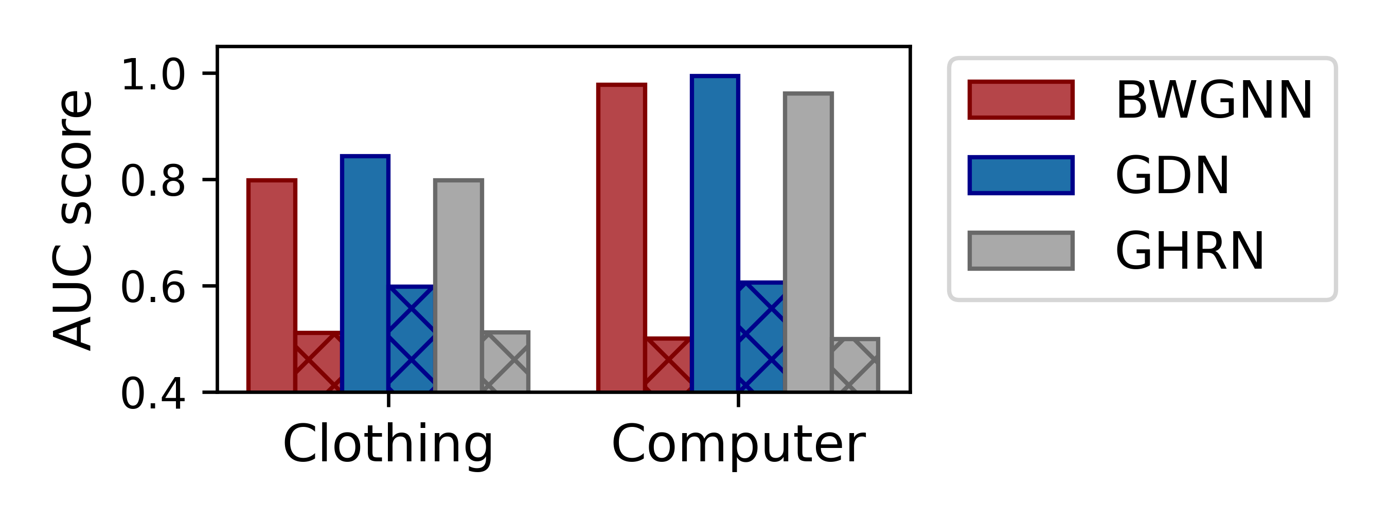
Figure 1: A pilot study reveals that noisy labels can degrade the performance of GAD models. The cross line denotes learning with noisy labels. See the experiment settings for details.

However, the performance of existing methods remains unsatisfactory to meet industrial needs. While they heavily rely on high-quality labels to facilitate supervised or semi-supervised learning, this hypothesis can hardly stand in real-world scenarios since the annotations are difficult to obtain. First, crowd-sourcing annotators can be unreliable in labeling the complex graph structure [16]. Ensuring high-quality labels requires careful data cleaning. Second, it is unaffordable to annotate extremely large graphs by involving human experts. In Fig.1, we showcase the impacts of noisy labels on two benchmark datasets. We stimulate the noise by label flipping in a heuristic way, and further details can be found in the Experiment Setting section. It is obvious that noisy labels significantly decline several semi-supervised detection models’ performance based on the metric of the area under the ROC curve. Consequently, noisy labels inevitably exist in the graphs[17]. The corresponding noise information would propagate through neighbors and affect the representation learning ability. A careful denoising method is urged for effective GAD.

we are motivated to cut the edges of suspicious nodes to alleviate the impact of noise during propagation. Nevertheless, this task is challenging since determining the noise candidates to be pruned is laborious. Given the large scale of real-world graphs, the search space is extremely big, making it difficult for the edge pruner to prioritize suspicious nodes. Moreover, it is hard to quantitatively evaluate the regret of cutting the edges which may bring either positive or negative influences. on one hand, we wish to cut as many suspicious nodes as possible. This over-prune may remove normal edges and result in a sparse structure, which may affect the graph learning ability. On the other hand, we require sufficient information by preserving enough edges, while an under-prune can hardly satisfy the purpose of noise mitigation.

To this end, we propose a novel policy-in-the-loop framework, the REinforced Graph Anomaly Detection model, i.e., REGAD, to learn from noisy labels for robust GAD effectively. Specifically, we aim to maximize the performance improvement (AUC) of a base detector by cutting noisy edges with an edge pruner. This is approximated through the nodes with a set of high-confidence labels generated by the pre-trained base detector since true labels are not readily available in the real world. (i) We design a tailored action and search space to train a policy network to carefully make decisions and cut the suspicious edges step by step, where only a few suspicious edges are prioritized in each step. (ii) We design a policy-in-the-loop mechanism to iteratively optimize the policy based on the feedback from the base detector, while the base detector correspondingly updates the sets of high-confidence labels based on the reconstructed graph structure by the edge pruner. The overall performance is evaluated by the cumulative rewards that have been received based on the performance (AUC).

In general, we summarize our contributions below:

1. We formally define the problem of noisy label learning for graph anomaly detection.

2. A tailored policy network is designed to carefully identify noisy labels and optimize the edge pruning by prioritizing the most suspicious nodes.

3. We design a novel policy-in-the-loop learning paradigm for GAD with noisy labels. GAD and the policy complementarily benefit each other to mitigate the impacts of noisy labels.

4. Extensive experiments are conducted to comprehensively demonstrate the superiority of our framework under 50% error rates on three datasets.

II Problem Statement

II-A Notation

We use $\mathcal{G}=(\mathcal{V,E},\mathrm{X})$ to denote an attributed graph, where $\mathcal{V}=\left\{v_{1},v_{2},...,v_{n}\right\}$ is the set of $n$ nodes, and $\mathcal{E}\subseteq\mathcal{V}\times\mathcal{V}$ is the set of edges. Besides, $\mathrm{X}=\left\{x_{1},x_{2},...,x_{n}\right\}$ is the node attributes, $\mathrm{X}\in\mathbb{R}^{n\times d}$, and $d$ is the attribute dimension. $\mathrm{A}\in\mathbb{R}^{n\times n}$ represents the adjacency matrix of $\mathcal{G}$. If $v_{i}$ and $v_{j}$ are connected, $\mathrm{A}_{ij}=1$. Otherwise, $\mathrm{A}_{ij}=0$. $\mathcal{V}_{L}=\left\{v_{1},v_{2},...,v_{l}\right\}$ represents labeled nodes, and $\mathcal{V}_{U}=\mathcal{V}-\mathcal{V}_{L}$ is the set of unlabeled nodes. $\mathcal{V}_{L}$ includes normal nodes $\mathcal{V}_{n}$ and abnormal nodes $\mathcal{V}_{a}$. In practice, we only obtain anomaly nodes $\mathcal{V}_{a}$ following $\left|\mathcal{V}_{a}\right|\ll\left|\mathcal{V}_{n}\right|$. $\mathcal{Y}_{L}=\left\{y_{1},y_{2},...,y_{l}\right\}$ denotes the real ground truth labels of $\mathcal{V}_{L}$. However, in our research problem, we assume they are not always trustworthy and correct and utilize $\bar{\mathcal{Y}}_{L}=\left\{\bar{y}_{1},\bar{y}_{2},...,\bar{y}_{l}\right\}$ to represent the noisy ground truth corrupted by noise.

II-B Problem Definition

Graph Anomaly Detection. Given an attributed graph $\mathcal{G}=(\mathcal{V,E},\mathrm{X})$, the GAD task is formulated as:

$$f(\mathcal{G},\mathcal{Y}_{L})\to\hat{\mathrm{S}},$$ (1)

where anomaly scores $\hat{\mathrm{S}}$ reflect the likelihood or degree of being an anomaly node. Higher $\hat{\mathrm{s}}_{i}$ means a higher possibility of being detected as an anomaly $v_{i}\in\mathcal{V}_{a}$. These predicted scores provide evidence to identify more anomaly nodes except existing $\mathcal{V}_{a}$ with high accuracy, especially in $\mathcal{V}_{U}$.

Graph Anomaly Detection with Noisy Labels. In this task, the ground truth labels $\bar{\mathcal{Y}}_{L}$ are not accurate, which means a small proportion of labeled nodes $\mathcal{V}_{L}$ are erroneously labeled. In noisy ground truth labels $\bar{\mathcal{Y}}_{L}$, $\bar{y}_{i}=0,i\in L$ is mistakenly labeled, so the real one is $y_{i}=1$. However, it is difficult to distinguish which is real from $\bar{\mathcal{Y}}_{L}$. Under this setting, we aim to predict correct matching anomaly scores $\hat{\mathrm{S}}$ for all nodes as much as possible supervised by $\bar{\mathcal{Y}}_{L}$, i.e.,

$$f(\mathcal{G}^{{}^{\prime}},\bar{\mathcal{Y}}^{{}^{\prime}}_{L})\to\hat{\mathrm{S}},$$ (2)

where the efficient detection model $f$ is to estimate the probabilities of nodes being anomalous. In contrast to classification tasks where multiple classes are considered, only two types, anomaly nodes $\mathcal{V}_{a}$ and normal nodes $\mathcal{V}_{n}$ are included in $\mathcal{V}_{L}$. Besides, labeled nodes are significantly smaller than the number of unlabeled nodes, denoted as $\left|\mathcal{V}_{L}\right|\ll\left|\mathcal{V}_{U}\right|$. To stimulate $\bar{\mathcal{Y}}_{L}$, we will use label flipping introduced in the experiment section in detail.

III Methodology

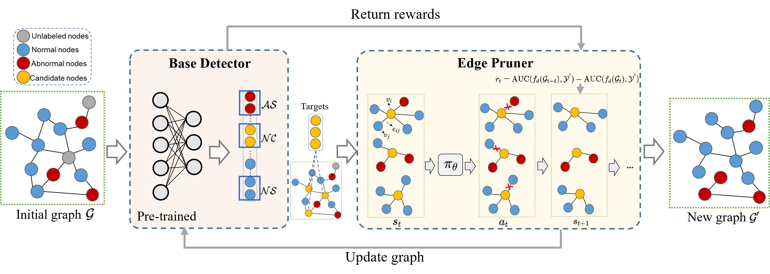
Figure 2: An overview of our framework REGAD. The base detector $f_{d}$ provides score predictions, determining two confident sets, i.e., $\mathcal{AS}$ and $\mathcal{NS}$ and candidate targets $\mathcal{NS}$ for the edge pruner. The edge pruner explores MDP to decide which edges to cut and balance the edge number by $\pi_{\theta}$ based on rewards.

In this section, we propose the REinforced Graph Anomaly Detection model in Fig. 2. Our model seeks to correct noisy truth labels and minimize the impact of noisy labels on neighborhood nodes based on the reinforcement learning method, designed as a policy-in-the-loop framework introduced in Section III-C. From the above targets, there are three challenges: 1) How can we identify noisy labels given that ground truths are not readily available? 2) Given the complicated graph structure, how can we control the negative impacts from nodes with noisy labels to their neighbors? 3) How can we quantitatively evaluate the influences of the edge pruner, i.e., positive (cut the real noisy edges) or negative (miscut edges)?

To address the first challenge, we employ a base detector to assess the anomaly score of each node supervised by noisy ground truth $\bar{\mathcal{Y}}_{L}$. It takes node attributes as the input and gives two confident node sets, anomaly set $\mathcal{AS}$, normal set $\mathcal{NS}$, and a noisy-label candidate set $\mathcal{NC}$. These candidates are the anchors in the following edge pruner, which is leveraged to solve the second challenge. To control incorrect information transmission, we apply reinforcement learning to learn a policy $\pi_{\theta}(a|s)$ to cut edges of candidates to manage noisy labels’ influence. Additionally, we employ the base detector performance based on the refined structure to evaluate the pruner quantitatively by returning rewards. These two components collaborate by exchanging information, forming the policy-in-the-loop framework. Next, each part is introduced in detail.

III-A Base Detector

The base detector $f_{d}$ is proposed to predict anomaly scores and generate pseudo labels, especially for unlabeled data supervised by noisy ground truth labels $\bar{\mathcal{Y}}_{L}$. Although we employ those training datasets, nodes with noisy labels, this detector could provide more information by predictions for unlabeled nodes. From this perspective, not all predictions are reliable, and thus we identify trustworthy anomaly set $\mathcal{AS}$, normal set $\mathcal{NS}$ for obtaining pseudo labels and modifying incorrect labels from score ranking. Nevertheless, due to supervision under noisy labels, the effective identification of candidates to be targeted by the pruner is made possible. To identify candidates $\mathcal{NC}$ for cutting edges and reduce noisy labels’ influence, we use a multi-armed bandit to determine which nodes are most likely to be candidates. Most candidates consist of erroneously labeled anomalous nodes hidden among the unlabeled ones, although there are also some normal nodes mislabeled as anomalous.

The base detector employs the Meta-GDN model [18] not only because it provides accurate scores and superior performance in GAD tasks but also because it addresses the issue of data imbalance [13, 18, 19, 20, 12] through balanced batches. Meta-GDN ensures that when using reliable sets for label rectification, the goal is to correct erroneous labels simultaneously, minimizing the production of incorrect labels. Additionally, based on the predicted scores ranking from Meta-GDN, candidates are identified using a multi-armed bandit approach to find the optimal pace deviated from mid-range scores, thereby locating nodes with potentially false labels. More importantly, rewards for the multi-armed bandit are designed based on the AUC corresponding to the selected nodes. As part of the iterative loop, Meta-GDN fulfills the aforementioned functions, updates node representations based on the refined graph, and calculates effective rewards for the pruner.

III-A1 Predict anomaly scores

The base detector maps node features into the low-dimensional latent space to learn node representations. We apply a simple Graph Convolutional Network (GCN) to provide node embeddings for score evaluation. To represent aggregation in one layer formally, the complete aggregation with an activation function of layer $l$ is formally written as:

$$\mathrm{H}^{l}=\sigma\left(\hat{\mathrm{A}}\mathrm{H}^{l-1}\mathrm{W}^{l-1}\right),$$ (3)

where $\hat{\mathrm{A}}=\tilde{\mathrm{D}}^{-1/2}\tilde{\mathrm{A}}\tilde{\mathrm{D}}^{-1/2}$ and $\tilde{\mathrm{A}}=\mathrm{A}+\mathrm{I}$. To clarify, $\mathrm{I}$ is an identity matrix and $\mathrm{D}$ is the degree matrix. $\sigma(\cdot)$ denotes an activation function, and the simplified expression is shown in Eq. 4. Graph neural networks are usually designed with several layers $L$ to keep the long-range information in the network. Finally, node representations $\mathrm{H}^{L}\in\mathbb{R}^{d\times r}$ are obtained, i.e.,

$$\mathrm{H}^{l}=GCN(\hat{\mathrm{A}},\mathrm{H}^{l-1}).$$ (4)

Given the above node embeddings, the detector evaluates an anomaly score for each node, namely the probability of being anomalous nodes. The score evaluation is composed of two simple linear layers as follows:

$$\hat{\mathrm{S}}=\mathrm{W}_{2}(\sigma(\mathrm{W}_{1}\mathrm{H}^{L}+b_{1}))+b_{2},$$ (5)

where $\hat{\mathrm{S}}$ denotes the predicted scores for all nodes and $\sigma(\cdot)$ is an activate function. $\hat{\mathrm{s}}_{i}$ denotes the score of node $v_{i}$. If $\hat{\mathrm{s}}_{i}\approx 1$ $v_{i}$ is anomalous, but if $\hat{\mathrm{s}}_{i}\approx 0$ node $v_{i}$ is more likely to be normal. However, if the score is difficult to discern labels $\hat{\mathrm{s}}_{i}\approx\bar{\mathrm{s}}$, $v_{i}$ has a high possibility to be a candidate with incorrect labels.

III-A2 Explore reliable sets and the candidate set

By ranking $\hat{\mathcal{S}}$, two high-confidence node sets are filtered out based on a hyper-parameter rate $\alpha$, i.e., anomaly set $\mathcal{AS}=\left\{v_{1},...v_{N_{as}}\right\}$ (the most suspicious), normal set $\mathcal{NS}=\left\{v_{1},...v_{N_{ns}}\right\}$ (the least suspicious). They are selected for label rectification to guarantee less noisy ground-truth labels:

$$\mathcal{AS} =\left\{v_{i}|\hat{\mathrm{s}}_{i}\in f_{top}^{\alpha}(\hat{\mathrm{S}})\right\},$$ (6)

$$\mathcal{NS} =\left\{v_{i}|\hat{\mathrm{s}}_{i}\in f_{top}^{\alpha}(-\hat{\mathrm{S}})\right\},$$ (7)

where $f_{top}$ is the node filtering function. Next, $\mathcal{AS}$ includes highly possible anomaly nodes, and thus ground truth labels $\bar{\mathcal{Y}}_{AS}$ should be updated as anomaly labels, i.e.,

$$\bar{\mathcal{Y}}^{{}^{\prime}}=\begin{cases}1&\text{ if }v_{i}\in\mathcal{AS};\\ 0&\text{ else if }v_{i}\in\mathcal{NS};\\ \bar{y}_{i}&\text{else,}\end{cases}$$ (8)

where $\bar{\mathcal{Y}}^{{}^{\prime}}$ denotes more reliable ground-truth labels than the noisy one $\bar{\mathcal{Y}}_{L}$, $\mathcal{NS}$ are normal node sets. Besides, the base detector is pre-trained for higher reliability to predict scores and update two sets.

Selecting a candidate set that may be anomalous from the remaining nodes is significant. Candidates directly determine the search space and quality of the pruner since a small proportion has incorrect labels. Therefore, we propose a method based on the multi-armed bandit algorithm $\mathcal{B}(A,f,T)$ to choose an appropriate threshold $\delta$ deviated from the mean value of the balanced batches’ anomaly scores. $A$ is the action space, $f$ is the reward function, and $T$ is the terminal condition. This threshold especially assists in restricting the score range of candidates, facilitating their edge-cutting as potential anomalies as:

$$\mathcal{NC}=\left\{v_{i}|\hat{\mathrm{s}}_{i}\in\bar{\mathrm{s}}\pm\delta\right\}$$ (9)

Concretely, we formulated the threshold selection based on $\epsilon$-greedy computation as the following steps:

• Action. In $t$-th iteration, a threshold value $\delta_{t}$ is randomly selected for exploration with a probability of $\epsilon$, while with a probability of (1-$\epsilon$), the current threshold is exploited.

  $$a_{t}=\begin{cases}\delta_{t},&\epsilon\\ argmax(\mathrm{AUC}(\hat{\mathrm{S}}_{\mathcal{NC}},\mathcal{Y}^{{}^{\prime}}_{\mathcal{NC}})),&1-\epsilon\end{cases}$$ (10)

• Reward. For each threshold $\delta_{t}$, the reward is the AUC value corresponding to the node candidate set whose scores fall within the range from $(\bar{\mathrm{s}}-\delta_{t})$ to $(\bar{\mathrm{s}}+\delta_{t})$. The reward value $r_{t}$ is computed by comparing candidates’ scores with the ground-truth labels as:

  $$r_{t}=\mathrm{AUC}(\hat{\mathrm{S}}_{\mathcal{NC}},\mathcal{Y}^{{}^{\prime}}_{\mathcal{NC}}),\delta=\delta_{t}$$ (11)

  To solve a special case with only one class, we randomly choose an anomaly node and one normal node to put in this candidate set to ensure reward computation.

• Terminal condition. The target is to minimize the candidate prediction performance, and lower AUC represents these nodes as the most noisy ones to be classified by the following process:

  $$T:r_{t}=min(f(\delta_{t})),t\leq N$$ (12)

Thereby, the base detector could facilitate REGAD in two folds: (i) updated ground-truth labels $\mathcal{Y}^{{}^{\prime}}$ provide confident supervision for GAD; (ii) the noisy candidate set $\mathcal{NC}=\left\{v_{1},...,v_{N_{nc}}\right\}$ guides the next edge pruner to reduce noisy information propagation.

III-B Edge Pruner

After determining the noisy candidate set $\mathcal{NC}$ from the base detector $f_{d}$, we leverage edge pruner $f_{e}$, as well as by reinforcement learning method, to remove edges centering nodes with noisy labels on the graph. The aim of the pruner is to learn a strategy to reshape the graph while keeping the semantic representation. The refined graph has more accurate pattern learning than before because edge-cutting prevents corrupted information transmission and leads to fewer nodes being corrupted from noisy ground-truth labels’ supervision. For normal nodes, edge-cutting has few negative effects since they typically have numerous edges connecting to other similar normal nodes. However, for anomaly nodes, cutting off edges around anomaly nodes highlights the impact of node features on score evaluation, reducing the assimilation of normal nodes. Thereby obtaining more accurate anomaly node patterns for direct detection.

Cutting edges to address noisy labels in graph structures is an effective way. However, the challenge of determining both the quality and quantity of selecting edges should be considered, as shown in Fig. 3. This example displays that cutting edges excessively risks some isolated nodes, while too few edges may fail to mitigate noisy information propagation. Faced with this difficulty, reinforcement learning [21, 22, 23] emerges as a promising approach due to efficient decision-making ability. Specifically, we utilize a policy network to learn the strategy of selecting functional edges, taking node representations as input. The output is the updated graph structure and the pruned edge set $\mathcal{E}_{cut}$.

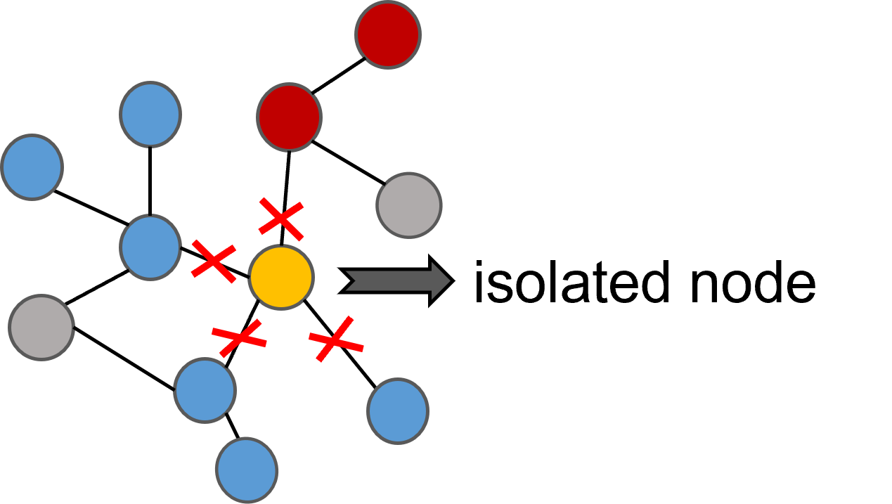
(a) Over-cutting

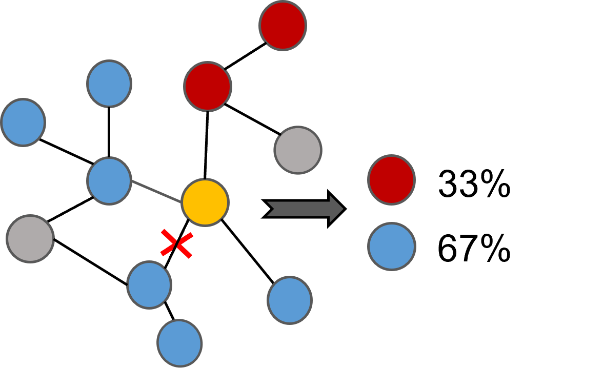
(b) Under-cutting

Figure 3: Possible scenarios resulting from improper pruning edges of candidates.

III-B1 Markov Decision Process

In this section, we reformulate the edge pruner module as a Markov Decision Process (MDP) to train a policy network. Specifically, an MDP is denoted as a tuple with $(\mathcal{S},\mathcal{A},\mathcal{P},\mathcal{R},\gamma)$, where $\mathcal{S}$ is the set of states, $\mathcal{A}$ is the set of actions, $\mathcal{P}$ is the state transition probability function, $\mathcal{R}$ is the reward function, and $\gamma$ is the discounting factor. Fig. 2 illustrates how the policy $\pi_{\theta}$ manipulates actions based on current states. The specification of each component is detailed as follows:

• State $\left(\mathcal{S}\right)$: In $t$-th step, state $s_{t}=(\hat{\mathrm{A}}_{t},\mathrm{H}_{t})$ is transitioned to the next state $s_{t+1}$. The initial state $s_{0}=(\hat{\mathrm{A}},\mathrm{H}^{L})$ comprises the adjacency matrix $\hat{\mathrm{A}}$ and the initial node representation $\mathrm{H}^{L}$ from the base detection.

• Action $(\mathcal{A})$: Given current state $s_{t}$, the agent selects action $a_{t}$ centered around candidate nodes in $\mathcal{NC}$ as below:

  $$a_{t}=\left\{e_{iN_{i}}^{t},...,e_{mN_{m}}^{t}\right\},N_{a}\leq n_{t}$$ (13)

  which includes $N_{a}$ edges of anchors simultaneously, but less than limitation $n_{t}$. The action space is stated as follows:

  $$\mathcal{E}_{\mathcal{NC}}=\left\{e_{ij},v_{i}\in\mathcal{NC},v_{j}\in N_{i}\right\},$$ (14)

  where $N_{i}$ denotes all neighbors of node $v_{i}$. Therefore, $a_{t}\subseteq\mathcal{E}_{\mathcal{NC}}$. Specifically, we utilize $\mathcal{E}_{T}=\sum_{t}^{T}a_{t}$ to aggregate all pruned edges in previous actions.

• Reward $(\mathcal{R})$: $r_{t}$ plays a vital role in guiding the agent to choose actions efficiently and correctly. Specifically, we compute reward $r_{t}$ by comparing detector performance before and after action $a_{t}$ based on the metric of AUC:

  $$r_{t}=\mathcal{R}(s_{t},a_{t},s_{t+1}).$$ (15)

The agent chooses the action $a_{t}$ with the given state $s_{t}$ and the MDP will transit to the next state $s_{t+1}$. The objective of the agent is to learn an optimal policy $\pi^{*}$ by solving:

$$\arg\max_{\theta}\mathbb{E}_{\pi_{\theta}}\left[\sum_{t=1}^{T}\gamma^{t}r_{t}|s_{0}\right],$$ (16)

where $s_{0}$ is the initial state of the MDP. The process of graph reconstruction can be depicted as a trajectory $\left\{s_{0},a_{1},r_{1},s_{1},a_{2},r_{2},...,s_{T}\right\}$, consisting of $T$ steps. This MDP could filter out the most optimal strategy, represented by a series of actions, to cut edges to reduce negative impacts of noisy labels.

III-B2 Policy Network Design

Having outlined the MDP above, we describe the architecture of the policy network determining action $a_{t}$. Given the current state $s_{t}$, the agent selects edges as action $a_{t}$ for all candidates to prune. The policy network consists of two GCN layers, as detailed below:

$$\mathrm{Z}_{t} =GCN(\hat{\mathrm{A}}_{t},\mathrm{H}_{t}),$$ (17)

$$\mathrm{P}_{t} =GCN(\mathrm{Z}_{t},\mathrm{H}_{t}),$$

where $GCN(\cdot)$ represents one GCN layer. $\hat{\mathrm{A}}_{t}$ and $\mathrm{H}_{t}$ are components of state $s_{t}$. The output $\mathrm{P}_{t}$ is a probability matrix, representing probabilities of edges being pruned. In the next stage, action $a_{t}$ is derived by selecting the top-k samples based on $\mathrm{P}_{t}$ for each candidate in $\mathcal{NC}$ as follows:

$$a_{t}=\bigcup_{v_{i}\in\mathcal{NC}}\text{Top}_{k}((\mathrm{P}_{t}\odot\mathrm{M})[i,:]),$$ (18)

where $\mathrm{P}_{t}[i,:]$ contains probabilities of edges connected to candidate $v_{i}$; $\mathrm{M}$ represents a mask matrix to exclude those pruned edges, where a value of 1 indicates that the edge is eligible for selection, and a value of 0 indicates that the edge is not eligible; $\text{Top}_{k}(\cdot)$ gives all existing top-k highest probabilities; $a_{t}$ aggregates selected edges for all nodes in $\mathcal{NC}$. This approach ensures that the edge selection process adheres to the constraints specified by the mask matrix $\mathrm{M}$.

III-B3 State Transition

Once the action $a_{t}$ is determined, the graph is updated by pruning selected edges in $a_{t}$. The state transition from $s_{t}$ to $s_{t+1}$ is written as:

$$s_{t+1}=\mathcal{P}_{a_{t}}(s_{t}),$$ (19)

which involves: 1) $\hat{\mathrm{A}}_{t}$ is modified by setting the element corresponding to the selected edges to zero, resulting in a new adjacency matrix $\hat{\mathrm{A}}_{t+1}$; 2) The node embeddings $\mathrm{H}_{t}$ are updated by passing the modified adjacency matrix $\hat{\mathrm{A}}_{t+1}$ through the base detection module. The new node embeddings $\mathrm{H}_{t+1}$ are stated as:

$$s_{t+1}=(\hat{\mathrm{A}}_{t}-a_{t},f_{d}(\hat{\mathrm{A}}_{t}-a_{t})).$$ (20)

III-B4 Reward Design

After the state transition, the reward $r_{t}$ is computed to evaluate the effectiveness of the action $a_{t}$. Specifically, The reward function $\mathcal{R}$ is defined by comparing detector performance, represented by results under the metric of AUC before and after action $a_{t}$ as:

$$r_{t}=\mathrm{AUC}(f_{d}(\mathcal{G}_{t+1}),\mathcal{Y}^{{}^{\prime}})-\mathrm{AUC}(f_{d}(\mathcal{G}_{t}),\mathcal{Y}^{{}^{\prime}})$$ (21)

where $\mathrm{AUC}(\cdot)$ calculates values by comparing truth labels and predicted scores. Most importantly, we utilize the confident updated truth labels $\mathcal{Y}^{{}^{\prime}}$ instead of noisy truth $\bar{\mathcal{Y}}_{L}$. Once the policy chooses action $a_{t}$, including multiple edges around anchor nodes, the new graph $\mathcal{G}_{t+1}$ can be easily obtained based on $s_{t+1}$. If the new graph performs better, $r_{t}$ is positive. Otherwise, the agent gets a negative reward.

III-C Policy-in-the-loop

The policy-in-the-loop frame is depicted as a cyclic framework where the base detector and pruner interact, providing necessary feedback to refine the graph structure. Concretely, the base detector assigns anomaly scores to detect anomalies according to graph structures, and the edge pruner manages to reconstruct the graph to address noisy information transmission, which allows the detector to prioritize anomaly pattern identification. In essence, edges linking normal nodes are mitigated and would lead to little influence due to numerous connections with other normal nodes. Conversely, edges around anomaly nodes have significant impacts because of limited edges.

III-C1 Policy Gradient Learning

The objective function is formulated to maximize the total reward during the Markov Decision Process (MDP) using the REINFORCE method, formulated as:

$$\mathcal{L}_{p}=-softmax(\sum_{t}^{T}\sum_{e_{ij}}^{\mathcal{E}_{T}}p_{t}^{e_{ij}}r_{t}\gamma_{t}),$$ (22)

where $\mathcal{L}_{p}$ denotes the loss incurred during training of the policy network and $p_{t}^{e_{ij}}$ is the probability value from matrix $\mathrm{P}_{t}$ corresponding to edge $e_{ij}$ in action $a_{t}$. $\gamma_{t}$ is the discount factor, and $r_{t}$ is the reward received at time step $t$.

Then, the training stage aims to update the policy network parameters $\theta$ using the policy gradient:

$$\theta\leftarrow\theta+\ell\cdot\bigtriangledown_{\theta}\mathcal{L}_{p},$$ (23)

where $\ell$ is the learning rate. The quantity of pruned edges is crucial as over-cutting may lead to numerous isolated nodes, while under-cutting may fail to reduce noisy information propagation. To address these issues, a terminal condition is set to ensure a balance in edge pruning and is terminated as:

$$N_{\mathcal{E}_{cut}}=\eta N_{nc},$$ (24)

where $N_{\mathcal{E}_{cut}}$ represents the total edge count in previous actions, and $N_{nc}$ is the number of nodes in $\mathcal{NC}$. $\eta$ denotes the rate to control the maximum number of pruned edges as a hyper-parameter. This ensures the policy network finds a balance in edge pruning to reduce the negative impacts of nodes with noisy labels.

IV Experiments

In this section, we conduct experiments to evaluate REGAD performance and answer the following questions:

• RQ1: How effective is the proposed method REGAD for anomaly detection under the noisy label setting?

• RQ2: What are the impacts of noisy label ratio on REGAD?

• RQ3: What are the performances of REGAD under different anomaly label numbers?

• RQ4: Is REGAD sensitive to the hyper-parameters?

• RQ5: How does our proposed method work in practice, especially the cutting-edge mechanism?

IV-A Experimental Settings

Datasets. We adopt three real-world attributed graphs that have been widely used in related studies in Table I. We follow the standard setup of graph anomaly detection research  [24, 25] and regard the nodes from the smallest class(es) as anomaly data (i.e., rare categories) while taking nodes from the other classes as ”normal” data. The details of three datasets are as follows:

• Clothing [26]: This dataset includes items such as clothing and jewelry from the Amazon website as nodes. The edges in this network represent instances in which two products are purchased together.

• Computer [27]: This dataset is a segment of the co-purchase graphs about computer-related items. Nodes represent individual device products, and edges represent frequent purchasing behaviors.

• Photo [27]: This dataset focuses on photography-related products, similar to the Computer dataset.

TABLE I: Statistics of datasets. $r$ denotes the anomaly ratio.

Datasets	Clothing	Computer	Photo
# Features	9,034	767	745
# Nodes	24,919	13,381	7,487
# Edges	91,680	245,778	119,043
# Anomalies	856	580	331
$r$	3.44%	4.33%	4.42%

Baselines. We compare the proposed method with three groups of methods for effectiveness evaluation, including (1) unsupervised GAD methods (e.g., DOM and ComGA), (2) semi-supervised GAD methods (e.g., Meta-GDN, DeepSAD, CHRN, BWGNN), (3) noisy label learning methods (e.g., D2PT, RTGNN, PIGNN). The details are as follows: DOM [28] is an unsupervised method including the decoder and encoder by reconstructing adjacent matrix to detect anomalies. ComGA [19] designs a community-aware method to obtain representations to predict anomaly scores. Meta-GDN [15] is the simple version of an anomaly detection model based on GCN leveraging balanced batch sizes and deviation loss between abnormal and normal nodes. DeepSAD [29] evaluates the entropy of the latent distribution for normal nodes and anomalous nodes to classify. BWGNN [20] is proposed to address the ’right-shift’ phenomenon of graph spectrum by Beta Wavelet Graph Neural Network. CHRN [13] addresses the heterophily of the GAD task by emphasizing high-frequency components by graph Laplacian. D2PT [30] innovates a dual-channel GNN framework, increasing robustness considering the augmented and original global graphs. RTGNN [31] focuses on noise governance by self-reinforcement supervision module and consistency regularization after graph augmentation. PIGNN [32] leverages structural pairwise interactions (PI) to propose a PI-aware model to manage noise.

Evaluation Metrics. Following previous papers [15, 33], we adopt two metrics, i.e., AUC and AUPR, that have been widely used for GAD. AUC denotes the area under the ROC curve, which illustrates the true positive rate against the false positive rate. AUPR is the area under the Precision-Recall curve, showing the trade-off between precision and recall.

Implementation Details. All datasets are split into training (40%), validation (20%), and test (40%) sets. Our research problem includes noisy labels, which are difficult to distinguish during the training and validation phase. However, current datasets are pre-processed and basically contain clean labels. To simulate the real-world scenarios of noisy labels, we follow related papers [34, 35] and induce noisy labels into the datasets with label flipping and then mix corrupted labels with correct ones. Specifically, Label flipping is a common method for introducing noisy labels, typically including uniform noise and pair noise, applied for node classification tasks. We generate noisy labels for anomaly detection by uniformly swapping normal nodes into the anomaly class at a designated rate.

In the experiments, if not further specified, the number of labeled anomalies is set to 30, and the noisy label ratio is 50%. Moreover, we adopt a pre-trained base detector with 2 layers of GCN with 128 hidden units to learn node representations and one linear layer to compute anomaly score predictions. Similarly, we leverage a 2-layer GCN as the policy network to manipulate edge-cutting strategies. The learning rate of the policy network is 0.005, and the weight decay is set to 5e-4. To make $\mathcal{AS}$ and $\mathcal{NS}$ more reliable, the rate $\alpha$ in Eq. 6 is a significant hyper-parameter ranging in [0.001, 0.1]. We also search the threshold $\delta$ to decide candidates with noisy labels in [0.1, 0.4] with 100 iterations. We filter out edges simultaneously, centering nodes in $\mathcal{NC}$ for the pruner. Edge sampling limitation $n_{t}$ of actions is set in [100, 150]. Episode $T$ to optimize the policy network ranges {5,10,15,20}. We train REGAD with 5 epochs to ensure stability. We run ten experiment runs and report the averaged results.

TABLE II: Performance comparison results under the noisy label ratio of 50%.

Methods	Clothing		Computer		Photo
	AUC	AUPR	AUC	AUPR	AUC	AUPR
DOM	0.502±0.001	0.015±0.000	0.500±0.002	0.020±0.000	0.494±0.005	0.021±0.0021
ComGA	0.537±0.015	0.041±0.002	0.539±0.017	0.047±0.002	0.481±0.026	0.060±0.060
BWGNN	0.512±0.003	0.044±0.003	0.501±0.002	0.044±0.001	0.501±0.002	0.045±0.001
GHRN	0.513±0.001	0.046±0.003	0.499±0.001	0.043±0.001	0.502±0.003	0.045±0.001
DeepSAD	0.559±0.013	0.150±0.009	0.533±0.057	0.066±0.043	0.914±0.008	0.452±0.045
Meta-GDN	0.598±0.047	0.094±0.010	0.605±0.095	0.261±0.024	0.876±0.020	0.421±0.007
RTGNN	0.501±0.015	0.034±0.002	0.397±0.018	0.033±0.001	0.524±0.018	0.046±0.002
D2PT	0.537±0.002	0.048±0.000	0.751±0.008	0.328±0.018	0.786±0.057	0.186±0.081
PIGNN	0.414±0.014	0.026±0.001	0.470±0.045	0.039±0.005	0.512±0.022	0.046±0.002
REGAD	0.678±0.006	0.092±0.003	0.754±0.005	0.357±0.014	0.930±0.006	0.486±0.027

IV-B Effectiveness Analysis (RQ1)

We present the results of AUC and AUPR in Table II and have the following observations: (1) Semi-supervised models (e.g., DeepSAD) marginally outperform the unsupervised models (e.g., ComGA). This suggests that supervised ground truth labels, even with noisy labels, can still guide learning abnormal patterns. (2) The noisy label learning GNN methods (e.g., RTGNN and D2PT) achieve sub-optimal performances on the GAD datasets compared with semi-supervised GAD models. It verifies that the existing GNNs that exploit noisy labels for node classification tasks are unsuitable for the GAD task. (3) The performance of our method REGAD significantly surpasses the baselines under the noisy label scenario. Inspired by semi-supervised and noisy label learning methods, REGAD relies less on truth labels and mitigates the influence of noisy labels from graph topology. This is because REGAD refines the graph structure to reduce noise propagation and rectifies incorrect labels simultaneously, which helps to provide accurate supervision for learning abnormal patterns in the policy-in-the-loop framework.

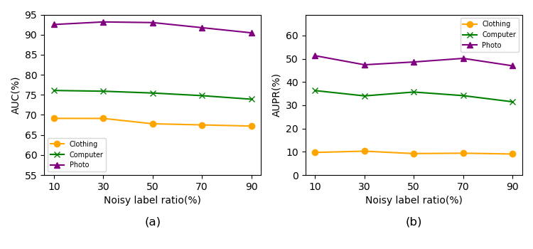
Figure 4: Impacts of noisy label ratios with fixed 30 anomaly labels on two metrics w.r.t. AUC and AUPR.

IV-C Analysis of Noisy Label Ratio (RQ2)

In this section, we implement experiments with different noisy label ratios, i.e., {10%, 30%, 50%, 70%, 90%} to analyze the robustness of REGAD. Firstly, we investigate the impacts of noisy label ratio under fixed labeled anomaly nodes. The corresponding number of nodes with clearly correct labels are {27,21,15,9,3} on three datasets. In Fig 4(a), we observe that the performance declines as the noisy label ratio increases. In addition, REGAD demonstrates effective detection results across different levels. Despite variations in the size and sparsity of datasets, REGAD’s performance remains consistent. The results are likely attributed to the ability of REGAD to effectively mitigate the influence of nodes with noisy labels on their neighboring nodes. Therefore, our model maintains relatively good results even under extremely noisy rate conditions.

In Fig. 4(b), the results based on the AUPR metric are presented. The overall trend of this curve is downward as the noisy label rate increases, which aligns with the expected noisy label impacts. However, fluctuations are observed: for instance, there is an initial increase followed by a continuous decrease from 30% to 50%, particularly in the Computer and Photo datasets. Introducing noisy labels within a proper range (30%-50%) may have a regularization effect, enabling the model to learn anomaly patterns better, thereby improving AUPR. Additionally, since the AUPR metric is more sensitive to predictions of minority classes, our model exhibits greater robustness at moderate noise-label rates. The Clothing dataset remains stable under different settings, which is attributed to REGAD’s effectiveness on sparse graphs.

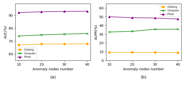
Figure 5: Impacts of anomaly nodes number with fixed noisy label ratio (50%) on two metrics w.r.t. AUC and AUPR.

IV-D Analysis of Labeled Anomaly Number (RQ3)

In this subsection, our main focus is to explore REGAD performance under different Anomaly label numbers. We set labeled anomaly nodes as {10, 20, 30, 40} respectively with a fixed noisy label ratio w.r.t. 50%. Under the AUC in Fig. 5(a), when labeled anomaly nodes increase, the performance of the three datasets improves. This is expected because a higher number of reliable anomaly labels provides more accurate supervised information. Even in extreme cases, such as with only 10 anomaly labels, REGAD achieves relatively good results. This indicates that rectifying some noisy ground truth labels and cutting edges can help mitigate noise in prediction collaboratively. The model exhibits a similar trend when evaluated using AUPR, except for the Photo dataset, where the performance decreases as labeled outliers increase. We speculate that increased labeled data can raise model complexity, particularly with many noisy labels, leading to overfitting of noisy-label nodes. Additionally, the cumulative effect of noise can hinder the ability of REGAD to extract useful information, resulting in decreased performance.

IV-E Sensitivity Analysis (RQ4)

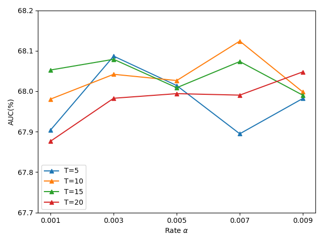
(a) $\alpha$ on Clothing

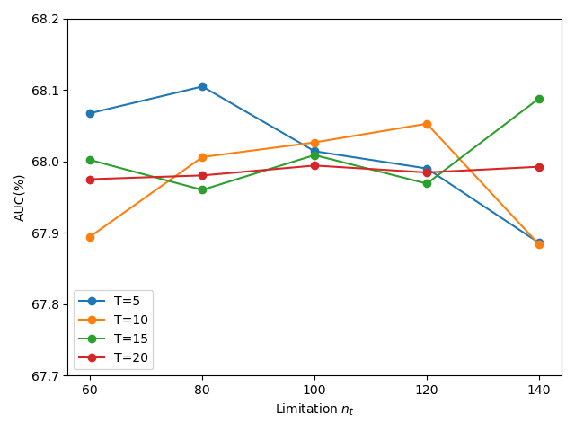
(b) $n_{t}$ on Clothing

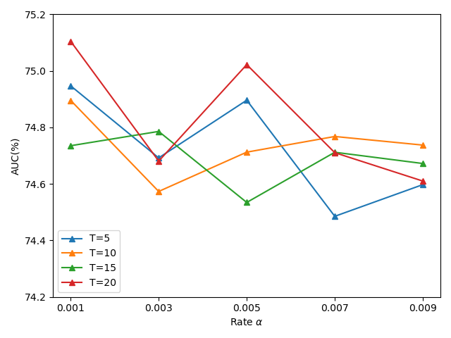
(c) $\alpha$ on Computer

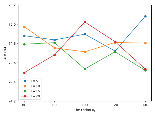
(d) $n_{t}$ on Computer

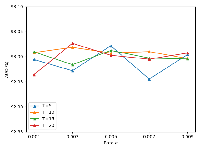
(e) $\alpha$ on Photo

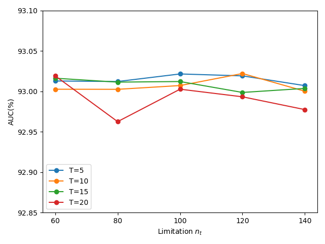
(f) $n_{t}$ on Photo

Figure 6: Sensitivity analysis of rate $\alpha$ and limitation $n_{t}$ on three datasets.

This section examines whether our model is sensitive to the three key hyper-parameters: (1) rate $\alpha$ determines rectified label rate; (2) limitation $n_{t}$ constrains edges chosen by each action. The results of three datasets are shown in Fig. 6 following the implementation setting (30 anomaly labels and 50% noisy labels). Furthermore, two parameters are set as {0.001, 0.003, 0.005, 0.007, 0.009}, {60,80,100,120,140} respectively. Specifically, in Fig. 6(a), Fig. 6(c), and Fig. 6(e), we can observe that REGAD is not very sensitive to these hyper-parameters, especially on the Photo dataset. For the $\alpha$, smaller values (e.g., 0.001-0.005) are generally recommended because $\alpha$ determines the proportion of labels directly modified based on the detector’s prediction. If the proportion is too high, it might introduce noise, requiring more actions to correct it, e.g., episode $T$=20. $n_{t}$ sets the maximum number of edges that can be chosen per action, allowing for a more gradual and controlled edge selection process in Fig. 6(b), Fig. 6(d), and Fig. 6(f). The value is recommended in the middle level (i.e., 80-100). Conversely, the limitation is widened to 140, and the performance falls sharply. This suggests our model’s stable and robust behavior, reaffirming its effectiveness across varied settings. In conclusion, findings underscore the reliability of REGAD in anomaly detection tasks.

IV-F Case Study (RQ5)

To further investigate how edge pruner functions effectively in REGAD, we analyze selected edges in actions of different episodes and epochs. This case study explores how the number of edges selected in each MDP varies across different episodes and epochs in Fig 7. We aim to understand how the pruner completes the graph construction process in several steps and whether the agent exhibits different strategies across episodes.

We observe some interesting phenomena. (1) The average cut edges have a small difference among epochs, indicating a stable performance within one epoch. (2) There is a significant variation of selected edges among different epochs. This variability is likely attributed to the process of policy optimization, where the model continuously explores different edge-pruning strategies. (3) Conversely, episodes within a single epoch tend to be more similar. The possible reason could be the model’s adaptation to newly learned patterns, which changes pruning decisions gradually. (4) The second action’s edges decrease noticeably across three datasets. This suggests that the agent can swiftly output edge-pruning actions with appropriate hyper-parameter settings, leading to a more efficient and effective MDP. In short, the listed examples reveal that REGAD refines graph structure to mitigate the influence of noisy labels for model learning and detecting anomaly nodes effectively.

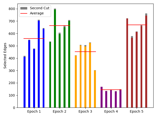
(a) Clothing dataset

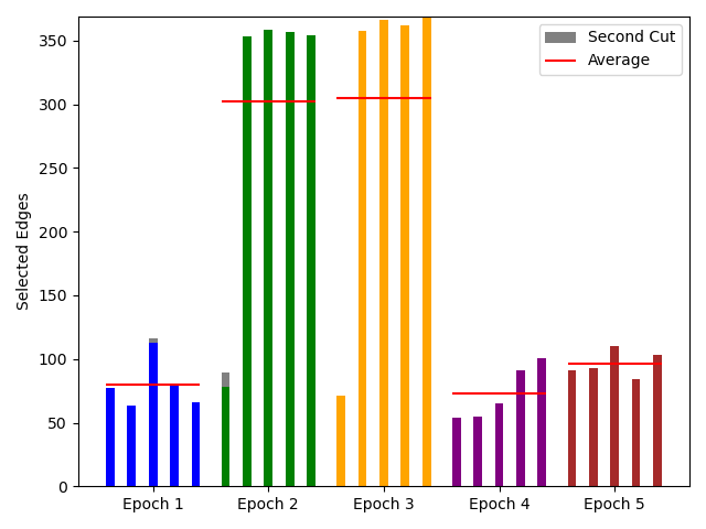
(b) Computer dataset

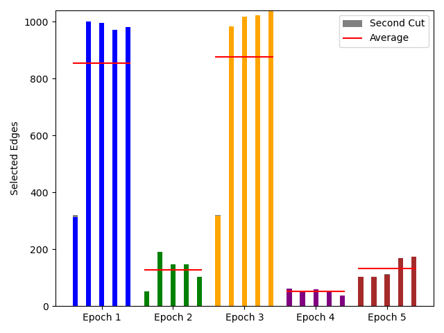
(c) Photo dataset

Figure 7: Example of selected edges 5 epochs in three datasets.

V Related work

V-A Graph Anomaly Detection

Graph anomaly detection (GAD) is a crucial task to identify graph objects that deviate from the main distribution [36, 37] with inherent connections and complex structures. Previous GAD methods roughly fall into three types: traditional, GNN-based, and hybrid methods.

Traditional methods [38] distinguish anomaly nodes from numerous nodes by learning feature patterns. Techniques including matrix factorization, KNN, and linear regression focus on evaluating similarity in the feature space. For example, [39] and [40] map normal nodes into a hyper-sphere, which filters out abnormal nodes outside that space. To achieve better detection performance, [20] and [18] converge on tackling the right-shift phenomenon of graph anomaly nodes. GNN-based methods [41, 42] utilize graph topology and manage neighborhood information, i.e., local node affinity [43]. A benchmark [44] illustrates that simple supervised ensembles with neighborhood aggregation also perform well on GAD. Unsupervised graph auto-encoder methods [28, 45] encode graphs and reconstruct graph structure by the decoder to detect anomalies. Some research leverages anomalous subgraphs [46] or duel channel GNN [13] to provide graph national causing abnormality and augment neighbors based on similarity. As for hybrid methods, approaches are applied in GNN-based methods such as meta-learning [15], contrastive learning [14, 4], and active learning [3]. This method’s biggest challenge is applying these deep-learning methods to instruct GAD. However, existing GAD methods often assume that clean and correct labels are available despite the expensive cost of confident annotations. Inspired by hybrid methods, this paper designs an effective detection model combined with reinforcement learning to address the challenge of noisy labels.

V-B Noisy Label Learning on Graph

The impact of noisy labels, including incomplete, inexact, and inaccurate labels in graphs, is relatively underexplored [47, 32, 35]. Graphs would render noisy information to truth labels and lead to poor detection performance. Current research endeavors meta-learning and augmentation to improve robustness. MetaGIN [48] obtains noise-reduced representations by interpolation and utilizes meta-learning to reduce label noise. Similarly, LPM [47] introduces meta-learning to optimize the label propagation, thereby reducing the negative effects of noisy information. RTGNN [31] and NRGNN [35] link unlabeled nodes with labeled nodes according to high similarity to augment graphs and predict pseudo labels for unlabeled nodes. Additionally, PIGNN [32] utilizes pair interactions, and D2PT [30] proposes dual channels of the initial graph to augment information to learn representations. However, the above methods are primarily designed for node classification tasks and may achieve sub-optimal performance for anomaly detection due to imbalanced distribution. Hence, we formulate the research problem of GAD with noisy labels that effectively leverage the available imperfect labels for effective anomaly detection.

V-C Graph Reinforcement Learning

Recent research has revolved around integrating Deep Reinforcement Learning (DRL) with GNN due to their complementary strengths in various tasks [49, 50], such as node classification with generalization. GraphMixup [51] and GraphSR [21] both employ reinforcement learning to augment minority classes by generating edges for unlabeled nodes, effectively addressing imbalanced data. Moreover, some research has explored the use of Reinforcement Learning for adversarial attacks in graph [52, 53] that employ generate virtual edges or detect attacked edges. However, designing effective reward functions remains challenging. Graph reinforcement learning is also utilized in tasks like explanation [23] and sparsification [54], identifying significant edges or prunes irrelevant ones. Furthermore, anomaly detection tasks based on the assumption of clean labels leverage RL to select and filter neighborhood information propagation in GNN [9, 55, 56], thereby simplifying anomaly node pattern learning. However, they consider all nodes as targets for information filtering, which poses a large search space for RL. These approaches are unsuitable for situations where noisy labels exist, especially in the case of imbalanced data. Since DRL has not yet been applied to address the issue of noisy labels, we tackle noisy label influence by selecting edges to reconstruct graph structure based on the policy-based method.

VI Conclusion

In this paper, we propose a policy-in-the-loop framework, REGAD, for the task of graph anomaly detection with noisy labels. We apply reinforcement learning to reconstruct graph structures, aiming to mitigate the negative impacts of noisy information by maximizing the AUC performance before and after reconstruction. Confident pseudo-labels are used as ground truth for suspicious labels to improve credibility. Experiments show that REGAD generally outperforms baseline methods on three datasets. REGAD demonstrates notable effectiveness, particularly with the edge pruner module on large datasets due to the smaller search space compared to typical models with reinforcement learning in the GAD task. Future work should focus on anomaly detection in sparse or complex graphs and selecting candidates from different base detectors by different standards.

References

- [1] Lizi Liao, Xiangnan He, Hanwang Zhang, and Tat-Seng Chua. Attributed Social Network Embedding. IEEE Transactions on Knowledge and Data Engineering, 30(12):2257–2270, December 2018.
- [2] Huachi Zhou, Shuang Zhou, Keyu Duan, Xiao Huang, Qiaoyu Tan, and Zailiang Yu. Interest driven graph structure learning for session-based recommendation. In Pacific-Asia Conference on Knowledge Discovery and Data Mining, pages 284–296. Springer, 2023.
- [3] Junnan Dong, Qinggang Zhang, Xiao Huang, Qiaoyu Tan, Daochen Zha, and Zhao Zihao. Active Ensemble Learning for Knowledge Graph Error Detection. In Proceedings of the Sixteenth ACM International Conference on Web Search and Data Mining, pages 877–885, Singapore, February 2023. ACM.
- [4] Qizhou Wang, Guansong Pang, Mahsa Salehi, Wray Buntine, and Christopher Leckie. Cross-Domain Graph Anomaly Detection via Anomaly-Aware Contrastive Alignment. In Proceedings of the AAAI Conference on Artificial Intelligence, pages 4676–4684, June 2023.
- [5] Yaqing Wang, Weifeng Yang, Fenglong Ma, Jin Xu, Bin Zhong, Qiang Deng, and Jing Gao. Weak Supervision for Fake News Detection via Reinforcement Learning. Proceedings of the AAAI Conference on Artificial Intelligence, 34(01):516–523, April 2020.
- [6] Jingyi Xie, Jiawei Liu, and Zheng-Jun Zha. Label Noise-Resistant Mean Teaching for Weakly Supervised Fake News Detection, June 2022.
- [7] Lu Cheng, Ruocheng Guo, Kai Shu, and Huan Liu. Causal Understanding of Fake News Dissemination on Social Media. In Proceedings of the 27th ACM SIGKDD Conference on Knowledge Discovery & Data Mining, KDD ’21, pages 148–157, New York, NY, USA, August 2021. Association for Computing Machinery.
- [8] Chuang Zhang, Qizhou Wang, Tengfei Liu, Xun Lu, Jin Hong, Bo Han, and Chen Gong. Fraud Detection under Multi-Sourced Extremely Noisy Annotations. In Proceedings of the 30th ACM International Conference on Information & Knowledge Management, ACM CIKM2021, pages 2497–2506, Virtual Event Queensland Australia, October 2021. ACM.
- [9] Yingtong Dou, Zhiwei Liu, Li Sun, Yutong Deng, Hao Peng, and Philip S. Yu. Enhancing Graph Neural Network-based Fraud Detectors against Camouflaged Fraudsters. In Proceedings of the 29th ACM International Conference on Information & Knowledge Management, CIKM2020, pages 315–324, Ireland, October 2020. ACM.
- [10] Chen Gao, Yu Zheng, Nian Li, Yinfeng Li, Yingrong Qin, Jinghua Piao, Yuhan Quan, Jianxin Chang, Depeng Jin, Xiangnan He, and Yong Li. A Survey of Graph Neural Networks for Recommender Systems: Challenges, Methods, and Directions. ACM Transactions on Recommender Systems, 1(1):1–51, March 2023.
- [11] Bo Han, Quanming Yao, Tongliang Liu, Gang Niu, Ivor W. Tsang, James T. Kwok, and Masashi Sugiyama. A Survey of Label-noise Representation Learning: Past, Present and Future, February 2021.
- [12] Yang Liu, Xiang Ao, Zidi Qin, Jianfeng Chi, Jinghua Feng, Hao Yang, and Qing He. Pick and Choose: A GNN-based Imbalanced Learning Approach for Fraud Detection. In Proceedings of the Web Conference 2021, WWW ’21, pages 3168–3177, New York, NY, USA, June 2021. Association for Computing Machinery.
- [13] Yuan Gao, Xiang Wang, Xiangnan He, Zhenguang Liu, Huamin Feng, and Yongdong Zhang. Addressing Heterophily in Graph Anomaly Detection: A Perspective of Graph Spectrum. In Proceedings of the ACM Web Conference 2023, pages 1528–1538, Austin TX USA, April 2023. ACM.
- [14] Jingcan Duan, Siwei Wang, Pei Zhang, En Zhu, Jingtao Hu, Hu Jin, Yue Liu, and Zhibin Dong. Graph Anomaly Detection via Multi-Scale Contrastive Learning Networks with Augmented View. In Proceedings of the AAAI Conference on Artificial Intelligence, volume 37, pages 7459–7467, June 2023.
- [15] Kaize Ding, Qinghai Zhou, Hanghang Tong, and Huan Liu. Few-shot Network Anomaly Detection via Cross-network Meta-learning. In Proceedings of the Web Conference 2021, WWW ’21, pages 2448–2456, New York, NY, USA, April 2021. Association for Computing Machinery.
- [16] Junnan Dong, Qinggang Zhang, Huachi Zhou, Daochen Zha, Pai Zheng, and Xiao Huang. Modality-Aware Integration with Large Language Models for Knowledge-based Visual Question Answering, March 2024.
- [17] Shengyuan Chen, Qinggang Zhang, Junnan Dong, Wen Hua, Qing Li, and Xiao Huang. Entity Alignment with Noisy Annotations from Large Language Models, May 2024.
- [18] Yuan Gao, Xiang Wang, Xiangnan He, Zhenguang Liu, Huamin Feng, and Yongdong Zhang. Alleviating Structural Distribution Shift in Graph Anomaly Detection. In Proceedings of the Sixteenth ACM International Conference on Web Search and Data Mining, pages 357–365, Singapore Singapore, February 2023. ACM.
- [19] Xuexiong Luo, Jia Wu, Amin Beheshti, Jian Yang, Xiankun Zhang, Yuan Wang, and Shan Xue. ComGA: Community-Aware Attributed Graph Anomaly Detection. In Proceedings of the Fifteenth ACM International Conference on Web Search and Data Mining, pages 657–665, Virtual Event AZ USA, February 2022. ACM.
- [20] Jianheng Tang, Jiajin Li, Ziqi Gao, and Jia Li. Rethinking Graph Neural Networks for Anomaly Detection. In Proceedings of the 39th International Conference on Machine Learning, pages 21076–21089. PMLR, June 2022.
- [21] Mengting Zhou and Zhiguo Gong. GraphSR: A Data Augmentation Algorithm for Imbalanced Node Classification. In AAAI. arXiv, February 2023.
- [22] Mrigank Raman, Aaron Chan, Siddhant Agarwal, Peifeng Wang, Hansen Wang, Sungchul Kim, Ryan Rossi, Handong Zhao, Nedim Lipka, and Xiang Ren. Learning to Deceive Knowledge Graph Augmented Models via Targeted Perturbation. In ICLR, ICLR2021. arXiv, May 2021.
- [23] Xiang Wang, Yingxin Wu, An Zhang, Fuli Feng, Xiangnan He, and Tat-Seng Chua. Reinforced Causal Explainer for Graph Neural Networks. IEEE Transactions on Pattern Analysis and Machine Intelligence, 45(2):2297–2309, February 2023.
- [24] Dawei Zhou, Jingrui He, Hongxia Yang, and Wei Fan. Sparc: Self-paced network representation for few-shot rare category characterization. In Proceedings of the 24th ACM SIGKDD International Conference on Knowledge Discovery & Data Mining, pages 2807–2816, 2018.
- [25] Shuang Zhou, Xiao Huang, Ninghao Liu, Huachi Zhou, Fu-Lai Chung, and Long-Kai Huang. Improving generalizability of graph anomaly detection models via data augmentation. IEEE Transactions on Knowledge and Data Engineering, 2023.
- [26] Kaize Ding, Jianling Wang, Jundong Li, Kai Shu, Chenghao Liu, and Huan Liu. Graph Prototypical Networks for Few-shot Learning on Attributed Networks. In Proceedings of the 29th ACM International Conference on Information & Knowledge Management, CIKM ’20, pages 295–304, New York, NY, USA, October 2020. Association for Computing Machinery.
- [27] Oleksandr Shchur, Maximilian Mumme, Aleksandar Bojchevski, and Stephan Günnemann. Pitfalls of Graph Neural Network Evaluation, June 2019.
- [28] Kaize Ding, Jundong LI, Rohit Bhanushali, and Huan Liu. Deep Anomaly Detection on Attributed Networks. In Proceedings of the 2019 SIAM International Conference on Data Mining, pages 594–602, Philadelphia, PA, May 2019. Society for Industrial and Applied Mathematics.
- [29] Lukas Ruff, Robert A. Vandermeulen, Nico Görnitz, Alexander Binder, Emmanuel Müller, Klaus-Robert Müller, and Marius Kloft. Deep Semi-Supervised Anomaly Detection. In International Conference on Learning Representations. arXiv, February 2020.
- [30] Yixin Liu, Kaize Ding, Jianling Wang, Vincent Lee, Huan Liu, and Shirui Pan. Learning Strong Graph Neural Networks with Weak Information. In Proceedings of the 29th ACM SIGKDD Conference on Knowledge Discovery and Data Mining, pages 1559–1571, August 2023.
- [31] Siyi Qian, Haochao Ying, Renjun Hu, Jingbo Zhou, Jintai Chen, Danny Z. Chen, and Jian Wu. Robust Training of Graph Neural Networks via Noise Governance. In Proceedings of the Sixteenth ACM International Conference on Web Search and Data Mining, WSDM ’23, pages 607–615, New York, NY, USA, February 2023. Association for Computing Machinery.
- [32] Xuefeng Du, Tian Bian, Yu Rong, Bo Han, Tongliang Liu, Tingyang Xu, Wenbing Huang, and Junzhou Huang. Noise-robust Graph Learning by Estimating and Leveraging Pairwise Interactions. Transactions on Machine Learning Research, pages 1–24, June 2021.
- [33] Shuang Zhou, Xiao Huang, Ninghao Liu, Qiaoyu Tan, and Fu-Lai Chung. Unseen anomaly detection on networks via multi-hypersphere learning. In Proceedings of the 2022 SIAM International Conference on Data Mining (SDM), pages 262–270. SIAM, 2022.
- [34] Yue Zhao, Guoqing Zheng, Subhabrata Mukherjee, Robert McCann, and Ahmed Awadallah. ADMoE: Anomaly Detection with Mixture-of-Experts from Noisy Labels. In AAAI2023, AAAI23. arXiv, November 2022.
- [35] Enyan Dai, Charu Aggarwal, and Suhang Wang. NRGNN: Learning a Label Noise-Resistant Graph Neural Network on Sparsely and Noisily Labeled Graphs. In Proceedings of the 27th ACM SIGKDD Conference on Knowledge Discovery & Data Mining, KDD ’21, pages 227–236, New York, NY, USA, August 2021. Association for Computing Machinery.
- [36] Minqi Jiang, Chaochuan Hou, Ao Zheng, Xiyang Hu, Songqiao Han, Hailiang Huang, Xiangnan He, Philip S. Yu, and Yue Zhao. Weakly Supervised Anomaly Detection: A Survey, February 2023.
- [37] Shuang Zhou. Graph anomaly detection with diverse supervision signals. 2024.
- [38] Xiaoxiao Ma, Jia Wu, Shan Xue, Jian Yang, Chuan Zhou, Quan Z. Sheng, Hui Xiong, and Leman Akoglu. A Comprehensive Survey on Graph Anomaly Detection with Deep Learning. IEEE Transactions on Knowledge and Data Engineering, 35(12):12012–12038, August 2021.
- [39] Xuhong Wang, Baihong Jin, Ying Du, Ping Cui, Yingshui Tan, and Yupu Yang. One-class graph neural networks for anomaly detection in attributed networks. Neural Computing and Applications, 33(18):12073–12085, September 2021.
- [40] Atsutoshi Kumagai, Tomoharu Iwata, and Yasuhiro Fujiwara. Semi-supervised Anomaly Detection on Attributed Graphs. In 2021 International Joint Conference on Neural Networks (IJCNN), pages 1–8, Shenzhen, China, July 2021. IEEE.
- [41] Kaize Ding, Jundong Li, and Huan Liu. Interactive Anomaly Detection on Attributed Networks. In Proceedings of the Twelfth ACM International Conference on Web Search and Data Mining, WSDM ’19, pages 357–365, New York, NY, USA, January 2019. Association for Computing Machinery.
- [42] Shuang Zhou, Qiaoyu Tan, Zhiming Xu, Xiao Huang, and Fu-lai Chung. Subtractive aggregation for attributed network anomaly detection. In Proceedings of the 30th ACM International Conference on Information & Knowledge Management, pages 3672–3676, 2021.
- [43] Hezhe Qiao and Guansong Pang. Truncated Affinity Maximization: One-class Homophily Modeling for Graph Anomaly Detection. In 37th Conference on Neural Information Processing Systems (NeurIPS 2023), 2023.
- [44] Jianheng Tang, Fengrui Hua, Ziqi Gao, Peilin Zhao, and Jia Li. GADBench: Revisiting and Benchmarking Supervised Graph Anomaly Detection. In 37th Conference on Neural Information Processing Systems (NeurIPS 2023), 2023.
- [45] Haoyi Fan, Fengbin Zhang, and Zuoyong Li. Anomalydae: Dual Autoencoder for Anomaly Detection on Attributed Networks. In ICASSP 2020 - 2020 IEEE International Conference on Acoustics, Speech and Signal Processing (ICASSP), pages 5685–5689, May 2020.
- [46] Yixin Liu, Kaize Ding, Qinghua Lu, Fuyi Li, Leo Yu Zhang, and Shirui Pan. Towards Self-Interpretable Graph-Level Anomaly Detection. In 37th Conference on Neural Information Processing Systems (NeurIPS 2023), 2023.
- [47] Jun Xia, Haitao Lin, Yongjie Xu, Lirong Wu, Zhangyang Gao, Siyuan Li, and Stan Z. Li. Towards Robust Graph Neural Networks against Label Noise. In Proceedings - ICLR 2021 Conference, ICLR2021, March 2021.
- [48] Kaize Ding, Jianling Wang, Jundong Li, James Caverlee, and Huan Liu. Robust Graph Meta-learning for Weakly-supervised Few-shot Node Classification, August 2022.
- [49] Mingshuo Nie, Dongming Chen, and Dongqi Wang. Reinforcement learning on graphs: A survey. IEEE Transactions on Emerging Topics in Computational Intelligence, January 2023.
- [50] Sai Munikoti, Deepesh Agarwal, Laya Das, Mahantesh Halappanavar, and Balasubramaniam Natarajan. Challenges and Opportunities in Deep Reinforcement Learning with Graph Neural Networks: A Comprehensive review of Algorithms and Applications, November 2022.
- [51] Lirong Wu, Jun Xia, Zhangyang Gao, Haitao Lin, Cheng Tan, and Stan Z. Li. GraphMixup: Improving Class-Imbalanced Node Classification by Reinforcement Mixup and Self-supervised Context Prediction. In Massih-Reza Amini, Stéphane Canu, Asja Fischer, Tias Guns, Petra Kralj Novak, and Grigorios Tsoumakas, editors, Machine Learning and Knowledge Discovery in Databases, Lecture Notes in Computer Science, pages 519–535, Cham, 2023. Springer Nature Switzerland.
- [52] Yiwei Sun, Suhang Wang, Xianfeng Tang, Tsung-Yu Hsieh, and Vasant Honavar. Adversarial Attacks on Graph Neural Networks via Node Injections: A Hierarchical Reinforcement Learning Approach. In Proceedings of The Web Conference 2020, WWW20, pages 673–683, Taipei Taiwan, April 2020. ACM.
- [53] Hanjun Dai, Hui Li, Tian Tian, Xin Huang, Lin Wang, Jun Zhu, and Le Song. Adversarial Attack on Graph Structured Data. In Proceedings of the 35th International Conference on Machine Learning, ICML2018, pages 1115–1124, July 2018.
- [54] Ryan Wickman, Xiaofei Zhang, and Weizi Li. A Generic Graph Sparsification Framework using Deep Reinforcement Learning. In 2022 IEEE International Conference on Data Mining (ICDM), ICDM2022, pages 1221–1226, November 2022.
- [55] Kaize Ding, Xuan Shan, and Huan Liu. Towards Anomaly-resistant Graph Neural Networks via Reinforcement Learning. In Proceedings of the 30th ACM International Conference on Information & Knowledge Management, CIKM ’21, pages 2979–2983, New York, NY, USA, October 2021. Association for Computing Machinery.
- [56] Mengda Huang, Yang Liu, Xiang Ao, Kuan Li, Jianfeng Chi, Jinghua Feng, Hao Yang, and Qing He. AUC-oriented Graph Neural Network for Fraud Detection. In Proceedings of the ACM Web Conference 2022, pages 1311–1321, Virtual Event, Lyon France, April 2022. ACM.