Abstract

We study the possibility of measuring T (time reversal) violation in a future long baseline neutrino oscillation experiment. By assuming a neutrino factory as a staging scenario of a muon collider at the J-PARC site, we find that the $\nu_{e}\to\nu_{\mu}$ oscillation probabilities can be measured with a good accuracy at the Hyper-Kamiokande detector. By comparing with the probability of the time-reversal process, $\nu_{\mu}\to\nu_{e}$, measured at the T2K/T2HK experiments, one can determine the CP phase $\delta$ in the neutrino mixing matrix if $|\sin(\delta)|$ is large enough. The determination of $\delta$ can be made with poor knowledge of the matter density of the earth as T violation is almost insensitive to the matter effects. The comparison of CP and T-violation measurements, à la the CPT theorem, provides us with a non-trivial check of the three neutrino paradigm based on the quantum field theory.

1 Introduction

The neutrino oscillation phenomena have provided us with the largest scale tests of the time evolution of physical states via quantum mechanics. The terrestrial experiments such as T2K [1] and NO$\nu$A [2] experiments are now operating to look for CP violating phenomena by using $O(100-1000)$ km size baselines. In future, such as within the time scale of ten years, Hyper-Kamiokande [3], JUNO [4] and DUNE [5] experiments are expected to uncover the oscillation parameters in the three neutrino scheme, such as the ordering of the neutrino masses and the size of the Dirac CP phase.

Once we know all of those, we can further ask interesting questions. Do neutrinos obey usual rules in the quantum mechanics? Do neutrinos have only weak interactions? Are there only three neutrino generations? It will be important to over-constrain the oscillation parameters to check if we really understand the lepton sector of the Standard Model, just as we have done to confirm the Kobayashi-Maskawa theory in the quark sector.

Of course, in the current situation, the discovery of CP violation in the neutrino sector itself will be the most important milestone. The standard method is to look for the difference in the $\nu_{\mu}\to\nu_{e}$ and $\bar{\nu}_{\mu}\to\bar{\nu}_{e}$ oscillations in the accelerator based long-baseline experiments [6]. Although observing the difference sounds a clear CP-violating signal, matter effects in the neutrino propagation in the earth make the analysis complicated as we need an anti-earth for the difference to be formally CP-odd. In other words, imperfect knowledge of the matter-density profile of the earth can fake the CP violation.

The importance of measuring T violation has been pointed out in Ref. [7, 8, 9]. Many physicists, say, in Ref [10, 11] considered the use of high intensity muon beams, so called neutrino factory [12]. The collimated $\nu_{e}$ flux from the muon decays in flight can be a good source for long baseline oscillation experiments. The observation of the $\nu_{e}\to\nu_{\mu}$ oscillation will be made possible in such experiments, and by comparing with $\nu_{\mu}\to\nu_{e}$, one can measure T violation. The virtue of T violation is that it is insensitive to the matter effects. Formally, the T violation is the difference between the oscillation probabilities of $\nu_{\mu}\to\nu_{e}$ and $\nu_{e}\to\nu_{\mu}$ while flipping the locations of source and the detector. By approximating the earth as a spherically symmetric object, the flipping would not change the probabilities, and thus one can perform the experiments by the same facility of the $\nu_{\mu}\to\nu_{e}$ measurements such as T2K and T2HK. It is also interesting to compare CP-violation measurements with T-violation ones. This is going to be a very non-trivial consistency check of the quantum mechanics of the three-neutrino paradigm.

Recently, neutrino-factory programs have been revived as a staging scenario of muon colliders (see for e.g., [13]). In Japan, there is a proposal to utilize the ultra slow muon technology [14] for muon cooling that is the essential part to realize a muon collider [15]. For example, one can use J-PARC as the proton driver to produce pions, and by catching almost all the pions as well as the muons from the pion decays, one can obtain $O(10^{14})$ cold positive muons per second. With this number, one can consider a high energy and high intensity $\mu^{+}e^{-}$ and $\mu^{+}\mu^{+}$ colliders, which are excellent Higgs boson factories. As one of the staging scenarios, one can consider a low energy $\mu^{+}$ beam such as $O(1)$ GeV for neutrino factory to shoot $\nu_{e}$ beams to Super/Hyper-Kamiokande. Indeed, the ultra slow muon technology has been used in the muon $g-2$/EDM experiment at J-PARC [16] to obtain a low-emittance and polarized muon beam which is to be accelerated up to about 200 MeV within the time scale of a few years.

In this paper, we study the possibility of measuring T violation in the long baseline experiments. As an example, we take the same baseline as the T2HK experiments, and assume the neutrino flux obtained from the number of muons mentioned above. We conduct $\chi^{2}$ analyses to evaluate the possibility of testing T violation.

This paper is organized as follows. In Section 2, we review neutrino oscillations in the three-flavor scheme, and discuss T and CP violation in neutrino oscillations. In Section 3, we conduct a statistical analysis to estimate the sensitivity of the long baseline experiment based on the $\nu_{e}$ beam from the neutrino factory to T violation defined as the probability difference. Section 4 is devoted to summary.

2 CP and T violation in neutrino oscillations

We explain here our notations used in this paper and derive formulae for CP and T violation in the oscillation probabilities. We present the energy dependencies of them and discuss the impacts of the matter effects.

We parametrize below the PMNS matrix which is a $3\times 3$ unitary matrix to relate the mass and flavor eigenstates in the lepton sector:

with the notation, $s_{ij}=\sin\theta_{ij}$ and $c_{ij}=\cos\theta_{ij}$. The time evolution of neutrinos is described by the following Schrödinger equation,

$$i\derivative{t}\matrixquantity(\nu_{e}(\bar{\nu}_{e})\\ \nu_{\mu}(\bar{\nu}_{\mu})\\ \nu_{\tau}(\bar{\nu}_{\tau})) =\mathcal{M}^{(\pm)}\matrixquantity(\nu_{e}(\bar{\nu}_{e})\\ \nu_{\mu}(\bar{\nu}_{\mu})\\ \nu_{\tau}(\bar{\nu}_{\tau})),$$ (1)

where we combined the equations for neutrinos ($\nu$) and anti-neutrinos ($\bar{\nu}$). The effective Hamiltonian in matter is given by

$$\mathcal{M}^{(\pm)}\equiv U^{(*)}\mathrm{diag}(0,\mathit{\Delta}E_{21},\mathit{\Delta}E_{31})U^{{\dagger}(T)}+\mathrm{diag}(\pm A,0,0).$$ (2)

where $\mathit{\Delta}E_{jk}\equiv\mathit{\Delta}m_{jk}^{2}/2E$ are the differences in the energy eigenvalues in vacua and $A=\sqrt{2}G_{F}n_{e}$ represents the matter effect. Here, the density of the electron in the earth, $n_{e}$, can be calculated from the matter density of the earth, $\rho$, which is in our analysis taken to be constant along the baseline for simplicity [17]. From this equation, we obtain expressions of the neutrino oscillation probabilities for a baseline length $L$ as

$$P(\nu_{\alpha}(\bar{\nu}_{\alpha})\to\nu_{\beta}(\bar{\nu}_{\beta}))=\delta_{\alpha\beta} -4\sum_{j>k}\mathrm{Re}\left[\tilde{U}^{(\pm)}_{\alpha j}\tilde{U}^{(\pm)*}_{\beta j}\tilde{U}^{(\pm)*}_{\alpha k}\tilde{U}^{(\pm)}_{\beta k}\right]\sin^{2}\left(\frac{\mathit{\Delta}\tilde{E}^{(\pm)}_{jk}L}{2}\right)$$

$$+2\sum_{j>k}\mathrm{Im}\left[\tilde{U}^{(\pm)}_{\alpha j}\tilde{U}^{(\pm)*}_{\beta j}\tilde{U}^{(\pm)*}_{\alpha k}\tilde{U}^{(\pm)}_{\beta k}\right]\sin\left(\mathit{\Delta}\tilde{E}^{(\pm)}_{jk}L\right)$$ (3)

where $\tilde{U}^{(\pm)}$ is the matrix diagonalizing $\mathcal{M}^{(\pm)}$ and $\tilde{E}^{(\pm)}_{jk}=\tilde{E}^{(\pm)}_{j}-\tilde{E}^{(\pm)}_{k}$, $\tilde{E}^{(\pm)}_{j}$ are eigenvalues of $\mathcal{M}^{(\pm)}$.

The CP violation in the neutrino oscillation can be defined as

$$P\quantity(\nu_{\alpha}\to\nu_{\beta})-P\quantity(\bar{\nu}_{\alpha}\to\bar{\nu}_{\beta})$$

$$=-4\sum_{j>k}\mathrm{Re}\left[\tilde{U}^{(+)}_{\alpha j}\tilde{U}^{(+)*}_{\beta j}\tilde{U}^{(+)*}_{\alpha k}\tilde{U}^{(+)}_{\beta k}\sin^{2}\left(\frac{\mathit{\Delta}\tilde{E}^{(+)}_{jk}L}{2}\right)-\tilde{U}^{(-)}_{\alpha j}\tilde{U}^{(-)*}_{\beta j}\tilde{U}^{(-)*}_{\alpha k}\tilde{U}^{(-)}_{\beta k}\sin^{2}\left(\frac{\mathit{\Delta}\tilde{E}^{(-)}_{jk}L}{2}\right)\right]$$

$$+2\sum_{j>k}\mathrm{Im}\left[\tilde{U}^{(+)}_{\alpha j}\tilde{U}^{(+)*}_{\beta j}\tilde{U}^{(+)*}_{\alpha k}\tilde{U}^{(+)}_{\beta k}\sin\left(\mathit{\Delta}\tilde{E}^{(+)}_{jk}L\right)-\tilde{U}^{(-)}_{\alpha j}\tilde{U}^{(-)*}_{\beta j}\tilde{U}^{(-)*}_{\alpha k}\tilde{U}^{(-)}_{\beta k}\sin\left(\mathit{\Delta}\tilde{E}^{(-)}_{jk}L\right)\right]$$ (4)

It is important to note that, even if the CP phase, $\delta$, is zero, this quantity does not necessarily vanish. This is due to the fact that CP transformation of matter should be anti-matter, and thus the quantity defined above is not quite CP-odd.

On the other hand, T violation can be defined as

$$P\quantity(\nu_{\alpha}\to\nu_{\beta})-P\quantity(\nu_{\beta}\to\nu_{\alpha}) =4\sum_{j>k}\mathrm{Im}\left[\tilde{U}^{(+)}_{\alpha j}\tilde{U}^{(+)*}_{\beta j}\tilde{U}^{(+)*}_{\alpha k}\tilde{U}^{(+)}_{\beta k}\right]\sin\left(\mathit{\Delta}\tilde{E}^{(+)}_{jk}L\right)$$

$$=4\tilde{J}^{(+)}\left[\sin\quantity(\mathit{\Delta}\tilde{E}^{(+)}_{12}L)+\sin\quantity(\mathit{\Delta}\tilde{E}^{(+)}_{23}L)+\sin\quantity(\mathit{\Delta}\tilde{E}^{(+)}_{31}L)\right]$$

$$=-16\tilde{J}^{(+)}\sin\quantity(\frac{\mathit{\Delta}\tilde{E}^{(+)}_{31}L}{}){2})\sin\quantity(\frac{\mathit{\Delta}\tilde{E}^{(+)}_{32}L}{}){2})\sin\quantity(\frac{\mathit{\Delta}\tilde{E}^{(+)}_{21}L}{}){2})$$ (5)

where $\tilde{J}^{(+)}\equiv\mathrm{Im}\left[\tilde{U}^{(+)}_{\alpha 1}\tilde{U}^{(+)*}_{\beta 1}\tilde{U}^{(+)*}_{\alpha 2}\tilde{U}^{(+)}_{\beta 2}\right]$ is the modified Jarlskog factor in matter [18, 19, 20]. It is known that this factor can be expressed in terms of the Jarlskog invariant in the vacuum, $J=s_{13}c_{13}^{2}s_{12}c_{12}s_{23}c_{23}\sin\delta$ [21, 22], as

$$\tilde{J}^{(\pm)}=\frac{\mathit{\Delta}E_{31}\mathit{\Delta}E_{32}\mathit{\Delta}E_{21}}{\mathit{\Delta}\tilde{E}^{(\pm)}_{31}\mathit{\Delta}\tilde{E}^{(\pm)}_{32}\mathit{\Delta}\tilde{E}^{(\pm)}_{21}}J.$$ (6)

T violation here is formally T-odd when we assume that the matter density is symmetric under the exchange of the neutrino source and the detector. Consequently, if $\delta$ is zero, the difference $P\quantity(\nu_{\alpha}\to\nu_{\beta})-P\quantity(\nu_{\beta}\to\nu_{\alpha})$ is also exactly zero. Therefore, when measuring $\delta$, T violation gives clearer signals [7].

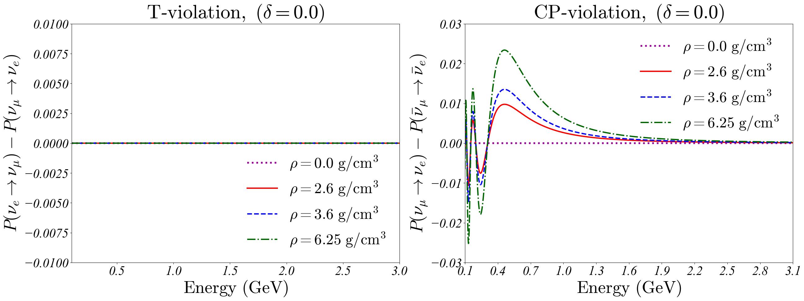
Figure 1: Energy dependence of T and CP violation for various choice of matter densities. The CP phase in the PMNS matrix is taken to be $\delta=0$. The purple dotted, red solid, blue dashed, and green dashdot lines correspond to $0.0~{}\rm{g/cm^{3}}$, $2.6~{}\rm{g/cm^{3}}$, $3.6~{}\rm{g/cm^{3}}$, $6.25~{}\rm{g/cm^{3}}$, respectively.

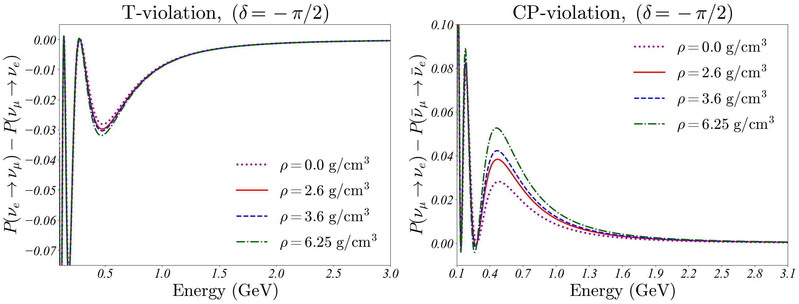
Figure 2: Energy dependence of T and CP violation for various choice of matter densities. The CP phase in the PMNS matrix is taken to be $\delta=-\pi/2$.

As a demonstration, we solve Eq. (1) for different matter densities, $\rho$, and show in Fig. 1 the energy dependence of the T and CP violation defined above for the case of $\delta=0$. It is clear that T violation vanishes while we see non-vanishing “CP violation,” which depend on the matter density $\rho$. This means, in order to establish the true CP violation, i.e., $\delta\neq 0$ nor $\pi$, via the measurements of the “CP violation,” we need good knowledge of matter profile in the earth. The same figure for $\delta=-\pi/2$ is shown in Fig. 2. We see a large dependence on the matter density in the case of CP violation, while T violation has essentially no difference. Although a little dependence shows up through the $\rho$ dependence in Eq. (6), one can see that complicated matter effects are largely removed in T violation measurements.

3 Statistical analysis

We discuss the statistical precisions of the CP and T violation measurement defined in the previous section. We assume a race-track type storage ring of the high-intensity muon beam at the J-PARC site with one of the straight section pointing towards the Hyper-Kamiokande detector. The decay of the beam muon produces a highly collimated neutrino beam and thus such a facility is referred-to as a neutrino factory [12]. Motivated by the discussion of muon collider experiments using the ultra slow muons ($\mu$TRISTAN), we assume a $\mu^{+}$ beam with a monochromatic energy at 1.5 GeV. The produced neutrinos are, therefore, $\bar{\nu}_{\mu}$ and $\nu_{e}$, with some energy distributions, which depends on the polarization of $\mu^{+}$. According to the estimates given in Ref. [15], the number of generated cold muons can be as large as $10^{14}$ per second even after considering all the efficiencies for muon stopping and laser ionizations. We expect that one can generate a few times $10^{21}$ per year in this type of facility. Since we assume a race-track type muon storage ring with two straight sections, we can make use of roughly 1/3 of muons whose decay products point to the far detector [23]. We expect that we are able to use $N_{\mu}=10^{21}/$year, and the total running time to be of the order of an year.

For the T-violation measurement, we use the $\nu_{e}$ beam to measure the oscillation probability $P(\nu_{e}\to\nu_{\mu})$ by comparing the number of $\nu_{e}$ produced at J-PARC and that of $\nu_{\mu}$ detected at Hyper-Kamiokande. The time-reversal probability, $P(\nu_{\mu}\to\nu_{e})$ is measured at the T2HK experiment by using the conventional beam from the pion ($\pi^{+}$) decays. We assume the same baseline for these two experiments. The CP violation, $P(\nu_{\mu}\to\nu_{e})-P(\bar{\nu}_{\mu}\to\bar{\nu}_{e})$ is also measured at the T2HK experiment.

For the measurement of $P(\nu_{e}\to\nu_{\mu})$, we need to distinguish $\nu_{\mu}$ from $\bar{\nu}_{\mu}$ at Hyper-Kamiokande as $\bar{\nu}_{\mu}$ is also produced by the decay of $\mu^{+}$. The water Cherenkov detector such as Hyper-Kamiokande can, in principle, identify the charge of the muons generated by the charged current process, $\nu_{\mu}n\to\mu^{-}p$ and $\bar{\nu}_{\mu}p\to\mu^{+}n$ by tagging the neutron in the final state, but the efficiencies of such signals are currently under studies [24, 25, 26]. We will discuss how we extract the oscillation probabilities under the $\bar{\nu}_{\mu}$ background later in this section.

3.1 Number of events at Hyper-Kamiokande

The neutrino flux from the neutrino factory can be estimated by the neutrino-energy ($E_{\nu}$) distribution of the (polarized) $\mu^{+}$ decay with a fixed energy $E_{\mu}$ [23]. By convoluting the $E_{\nu}$ distribution with the oscillation probabilities, $P^{\nu_{e}\to\nu_{\mu}}(E_{\nu})$, and the cross section of the neutrino-nucleon scattering, $\sigma_{\nu_{\mu}}(E_{\nu})$, one can obtain the event rate in each energy bin. The number of events is given by

$$N_{j}^{\nu_{e}\to\nu_{\mu}} =\int_{E_{j}}^{E_{j+1}}\frac{dE_{\nu}}{E_{\mu}}\times\frac{12N_{\mu}\cdot V\cdot n_{N}}{\pi L^{2}}\times\gamma^{2}\quantity(\frac{E_{\nu}}{E_{\mu}})^{2}\times\quantity[\quantity(1-\frac{E_{\nu}}{E_{\mu}})-P_{\mu}\quantity(1-\frac{E_{\nu}}{E_{\mu}})]$$

$$\times P^{\nu_{e}\to\nu_{\mu}}(E_{\nu})\times\sigma_{\nu_{\mu}}(E_{\nu}).$$ (7)

where $V$ is the detector volume, $n_{N}$ is the number density of the nucleon in water, and $L$ is the length of the baseline. The boost factor $\gamma$ is that for the muon, i.e., $\gamma=E_{\mu}/m_{\mu}$ with $m_{\mu}$ the muon mass. We assume a polarization of the anti-muon beam $P_{\mu}$ which is possible in the scheme of the ultra slow muon. The polarization will be important to obtain a larger $\nu_{e}$ flux in the forward region. Since we are going to perform combined analyses with the T2HK experiment, the far detector is assumed to be Hyper-Kamiokande and the baseline length is $L=295\ \mathrm{km}$. We show in Fig. 3 the number of events, $N_{j}^{\nu_{e}\to\nu_{\mu}}$ for a choice of the CP-phase $\delta=-\pi/2$ (red solid) and $\delta=0$ (red dashed) for $P_{\mu}=-1.0$, $-0.5$, $0.0$, and $+0.5$ for anti-muon. We also overlaid the number of background events, $N_{j}^{\bar{\nu}_{\mu}\to\bar{\nu}_{\mu}}$ (blue solid and dashed). Near the energy region $E_{\nu}\sim 0.5-0.7$ GeV, the background events are suppressed since that is the energy for the oscillation maximum for $L=295$ km. This is quite fortunate situation as the signal events (red) have a peak near such energies. We also see that the number of events are the largest for $P_{\mu}=-1.0$. At this stage, one can expect that the measurement of the $\nu_{e}\to\nu_{\mu}$ process will be possible with a neutrino factory at J-PARC with $N_{\mu}=10^{21}$/year. We use the cross section data for charged current quasielastic interactions from Ref. [27].

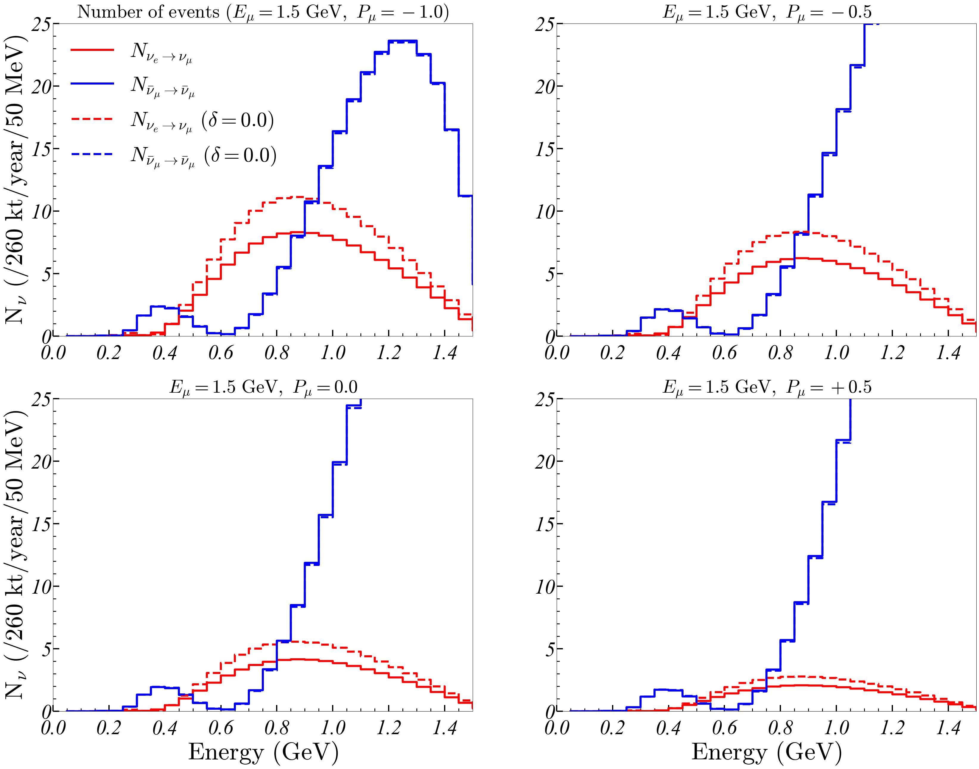
Figure 3: Neutrino flux measured at the far detector. The anti-muon beam energy is set to $1.5~{}\mathrm{GeV}$, and calculations are performed for four polarizations ($P_{\mu}=-1.0,\ -0.5,\ 0.0,\ +0.5$). The solid (dashed) lines depict the fluxes for $\delta=-\pi/2$ ($\delta=0.0$).

We also show in Fig. 4 the expected number of events for the CP-violation measurements, $N_{j}^{\nu_{\mu}\to\nu_{e}}$ and $N_{j}^{\bar{\nu}_{\mu}\to\bar{\nu}_{e}}$ in the T2HK experiment. We use the neutrino flux calculated in Ref. [3]. We see much larger event rates than the neutrino factory cases thanks to the large neutrino flux of the conventional beam.

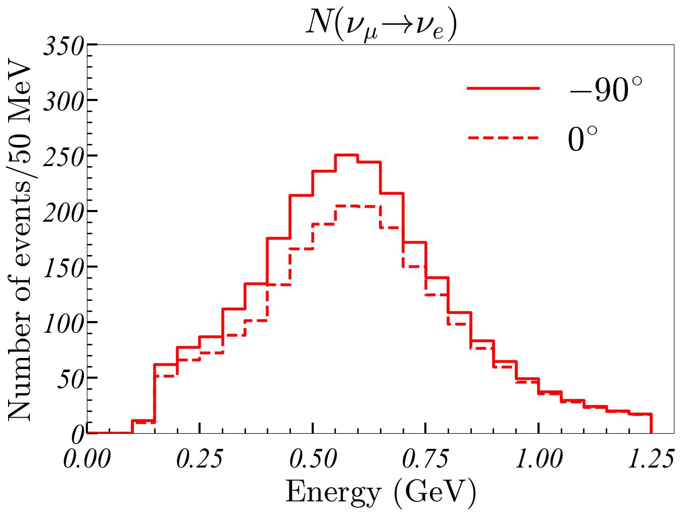
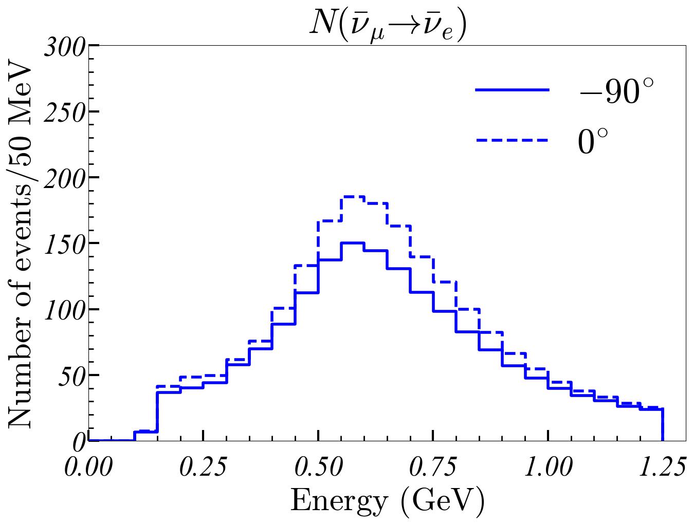
Figure 4: Number of events in the T2HK experiment. The left and right figures show the fluxes of $\nu_{\mu}\to\nu_{e}$ and $\bar{\nu}_{\mu}\to\bar{\nu}_{e}$ at the far detector, respectively. The solid (dash) lines correspond to $\delta=$$\ (\delta=$$)$. These expected number of events are taken from Ref. [3].

3.2 Background subtraction

As we see above, we have background events from $\bar{\nu}_{\mu}\to\bar{\nu}_{\mu}$ for the measurement of $N^{\nu_{e}\to\nu_{\mu}}$. The method of the neutron tagging can in principle distinguish $\nu_{\mu}$ from $\bar{\nu}_{\mu}$ but the detail efficiencies are not known at this stage. As a reference, the efficiency of the charge identification is about 70% at SK-Gd, and it is going to be better at Hyper-Kamiokande. In this study, we study the cases with various efficiencies of charge identification ($C_{\rm id}$), such as the most optimistic choice $C_{\rm id}=100\%$, middle $C_{\rm id}=70\%$, and the pessimistic one $C_{\rm id}=0\%$. For simplicity, we assume the efficiencies to be independent of the neutrino energy. We further assume that, by the time of the T2HK experiment to be being conducted, $C_{\rm id}$ is measured and known. In this situation, by simply subtracting the known $\bar{\nu}_{\mu}$ flux multiplied by the known misidentification rate, one can obtain the pure event rate $N^{\nu_{e}\to\nu_{\mu}}$.

In this method, the oscillation probability, $P(\nu_{e}\to\nu_{\mu})$, at each energy bin can be defined as

$$P(\nu_{e}\to\nu_{\mu})={1\over\kappa}\frac{\quantity(\kappa N_{\rm far}^{\nu_{e}\to\nu_{\mu}}+(1-\kappa)N_{\rm far}^{\bar{\nu}_{\mu}\to\bar{\nu}_{\mu}})-(1-\kappa)N_{\rm far}^{\bar{\nu}_{\mu}\to\bar{\nu}_{\mu}}\big{|}_{\rm T2HK}}{N_{\rm near}^{\nu_{e}\to\nu_{e}}},$$ (9)

and

$$\kappa \equiv\frac{1+C_{\rm id}}{2}.$$ (10)

Here, $N_{\rm near}$ and $N_{\rm far}$ denote the number of events at the source and at the detector, respectively, while $N_{\rm near}$ is corrected by the factor of the detector volume so that $N_{\rm far}/N_{\rm near}$ gives the probabilities. The factor $\kappa$ represents the probability to correctly identify $\nu_{\mu}$ for an actual $\nu_{\mu}$ event, while $1-\kappa$ is the misidentification probability. Therefore, the combination, $\kappa N_{\rm far}^{\nu_{e}\to\nu_{\mu}}+(1-\kappa)N_{\rm far}^{\bar{\nu}_{\mu}\to\bar{\nu}_{\mu}}$, is the actual number of events to be observed. On the other hand, $N_{\rm far}^{\bar{\nu}_{\mu}\to\bar{\nu}_{\mu}}\big{|}_{\rm T2HK}$ is the expected number of background events calculated based on the knowledge of $P(\bar{\nu}_{\mu}\to\bar{\nu}_{\mu})$ measured at the T2HK experiment.

For $C_{\rm id}=0$, i.e., $\kappa=0.5$, it is not sensible to perform the charge identification analysis since it is just the same as the random choices of the events, while we lose a half of the signal events by the selection. In the following analysis, when we take $C_{\rm id}=0$, we just do not perform the charge identification analysis and simply add the background events, and subtract the estimated amount by using the T2HK data, i.e., we take $\kappa=1$ and $1-\kappa=1$ in Eq. (9).

3.3 Statistical uncertainties

Combining $P(\nu_{e}\to\nu_{\mu})$ defined in Eq. (9) with the oscillation probability $P(\nu_{\mu}\to\nu_{e})$ measured at the T2HK experiment, one can now obtain the T-violation in Eq. (5) for each energy bin labeled by $j$ such as

$$P_{j}^{\rm TV}=P_{j}(\nu_{e}-\nu_{\mu})-P_{j}(\nu_{\mu}-\nu_{e})\big{|}_{\rm T2HK},$$ (11)

where the first term is defined in Eq. (9) and the latter term is the time reversal probability measured at the T2HK experiment. We discuss here the $\chi^{2}$ analysis to estimate the expected accuracy of the measurements.

In defining $\chi^{2}$, we take the CP phase $\delta$ as well as the matter density $\rho$ as the input parameters, and discuss how well we can measure $\delta$. Although the matter density of the earth, $\rho$, may be inferred by some other methods, we simply take the attitude that we do not know the actual value. By doing so, one can demonstrate how $\rho$ affects the measurement of $\delta$ and how T violation is insensitive to the matter profile.

For the rest of oscillation parameters, we take the following reference values, which correspond to the arithmetic average of the best fit points in Ref. [28] from three groups. In this study, we consider only the case of NO (Normal Ordering) for illustration.

$\mathit{\Delta}m_{21}^{2}/10^{-5}\ \mathrm{eV}$	$\mathit{\Delta}m_{31}^{2}/10^{-3}\ \mathrm{eV}$	$\theta_{12}$	$\theta_{13}$	$\theta_{23}$
$7.43$	$2.432$	$33.9\mathrm{°}$	$8.49\mathrm{°}$	$48.1\mathrm{°}$

Table 1: The reference values of oscillation parameters for the normal mass ordering.

When we take the true values for the input parameters as $\delta_{0}$ and $\rho_{0}$, $\chi^{2}$ for the T-violation measurement as a function of postulated values of $\delta=\delta^{\rm test}$ and $\rho=\rho^{\rm test}$ is defined as

$$\chi^{2}_{\rm TV}(\delta^{\rm test},\rho^{\rm test}) \equiv\sum_{j}\frac{\quantity[P^{\rm TV}_{j}\quantity(\delta_{0},\ \rho_{0})-P^{\rm TV}_{j}\quantity(\delta^{\rm test},\ \rho^{\rm test})]^{2}}{\quantity(\mathit{\Delta}P^{T\rm V}_{j})^{2}}$$ (14)

where $j$ runs over energy bins. Although we use the probability difference $P^{\rm TV}_{j}$ as the observable in this definition, the actual measurements are of course based on counting of $(\kappa N_{\rm far}^{\nu_{e}\to\nu_{\mu}}+(1-\kappa)N_{\rm far}^{\bar{\nu}_{\mu}\to\bar{\nu}_{\mu}})_{j}$ at the neutrino factory to Hyper-Kamiokande experiment and $(N_{\rm far}^{\bar{\nu}_{\mu}\to\bar{\nu}_{\mu}})_{j}\big{|}_{\rm T2HK}$ as well as $(N_{\rm far}^{\nu_{\mu}\to\nu_{e}})_{j}\big{|}_{\rm T2HK}$ at the T2HK experiment as it is clear in the defining equation in Eqs. (9) and (11).

Accordingly, the statistical error $\mathit{\Delta}P^{\rm TV}_{j}$ is given by

$$\quantity(\mathit{\Delta}P^{\rm TV}_{j})^{2} =\quantity(\mathit{\Delta}P_{j}^{\nu_{e}\to\nu_{\mu}})^{2}+\quantity(\mathit{\Delta}P_{j}^{\nu_{\mu}\to\nu_{e}})^{2}$$

$$=(P_{j}^{\nu_{e}\to\nu_{\mu}})^{2}\quantity{{\quantity(\frac{\mathit{\Delta}\quantity(\kappa N^{\nu_{e}\to\nu_{\mu}}_{\rm far}+(1-\kappa)N^{\bar{\nu}_{\mu}\to\bar{\nu}_{\mu}}_{\rm far})}{\kappa N^{\nu_{e}\to\nu_{\mu}}_{\rm far}})_{j}^{2}}+\quantity(\frac{\mathit{\Delta}N^{\nu_{e}\to\nu_{e}}_{\rm near}}{N^{\nu_{e}\to\nu_{e}}_{\rm near}})_{j}^{2}}$$

$$+(P_{j}^{\nu_{\mu}\to\nu_{e}})^{2}\quantity{\quantity(\frac{\mathit{\Delta}N^{\nu_{\mu}\to\nu_{e}}_{\rm far}}{N^{\nu_{\mu}\to\nu_{e}}_{\rm far}})^{2}_{j}+\quantity(\frac{\mathit{\Delta}N^{\nu_{\mu}\to\nu_{\mu}}_{\rm near}}{N^{\nu_{\mu}\to\nu_{\mu}}_{\rm near}})_{j}^{2}}$$

$$=(P_{j}^{\nu_{e}\to\nu_{\mu}})^{2}\quantity{{\quantity(\frac{\sqrt{\quantity(\kappa N^{\nu_{e}\to\nu_{\mu}}_{\rm far}+(1-\kappa)N^{\bar{\nu}_{\mu}\to\bar{\nu}_{\mu}}_{\rm far})}}{\kappa N^{\nu_{e}\to\nu_{\mu}}_{\rm far}})_{j}^{2}}+\quantity(\frac{\sqrt{N^{\nu_{e}\to\nu_{e}}_{\rm near}}}{N^{\nu_{e}\to\nu_{e}}_{\rm near}})_{j}^{2}}$$

$$+(P_{j}^{\nu_{\mu}\to\nu_{e}})^{2}\quantity{\quantity(\frac{\sqrt{N^{\nu_{\mu}\to\nu_{e}}_{\rm far}}}{N^{\nu_{\mu}\to\nu_{e}}_{\rm far}})^{2}_{j}+\quantity(\frac{\sqrt{N^{\nu_{\mu}\to\nu_{\mu}}_{\rm near}}}{N^{\nu_{\mu}\to\nu_{\mu}}_{\rm near}})_{j}^{2}}$$

$$\sim(P_{j}^{\nu_{e}\to\nu_{\mu}})^{2}{\quantity(\frac{\sqrt{\quantity(\kappa N^{\nu_{e}\to\nu_{\mu}}_{\rm far}+(1-\kappa)N^{\bar{\nu}_{\mu}\to\bar{\nu}_{\mu}}_{\rm far})}}{\kappa N^{\nu_{e}\to\nu_{\mu}}_{\rm far}})_{j}^{2}}+(P_{j}^{\nu_{\mu}\to\nu_{e}})^{2}\quantity(\frac{\sqrt{N^{\nu_{\mu}\to\nu_{e}}_{\rm far}}}{N^{\nu_{\mu}\to\nu_{e}}_{\rm far}})^{2}_{j}$$ (15)

Here, we assume that the number of events to obey the Gaussian distribution, and the variances of each observables are simply added to obtain the total uncertainty as each measurement is supposed to be independent. While we use the same notation $N_{\rm near}$ as in Eq. (9), $N_{\rm near}$ in Eq. (9) is actually different from $N_{\rm near}$ in Eq. (15). In Eq. (15), $N_{\rm near}$ is the value before applying corrections for distance and detector volume. This is because the applied corrections are known, and the number of events observed is before the corrections are applied. Therefore, the uncorrected number of events should be used for error evaluation. In any case, however, since $N_{\rm near}$ in Eq. (15) is much larger than $N_{\rm far}$, the contribution of this part is negligible, and the final expression does not contain $N_{\rm near}$.

By using the above estimated errors in each energy bin, we present the expected accuracy of the T-violation measurements in Fig. 5 ($\delta_{0}=-\pi/2$, $\rho_{0}$ = 2.6 g/cm³) and in Fig. 6 ($\delta_{0}=0.0$, $\rho_{0}$ = 2.6 g/cm³). We take the bin size to be 50 MeV, and take the polarization factor $P_{\mu}$ to be $-1.0$, $-0.5$, and $0.0$ (from left to right). The efficiency of the charge identification, $C_{\rm id}$ is taken to be $1.0$, $0.7$ and $0.0$ (from top to bottom).

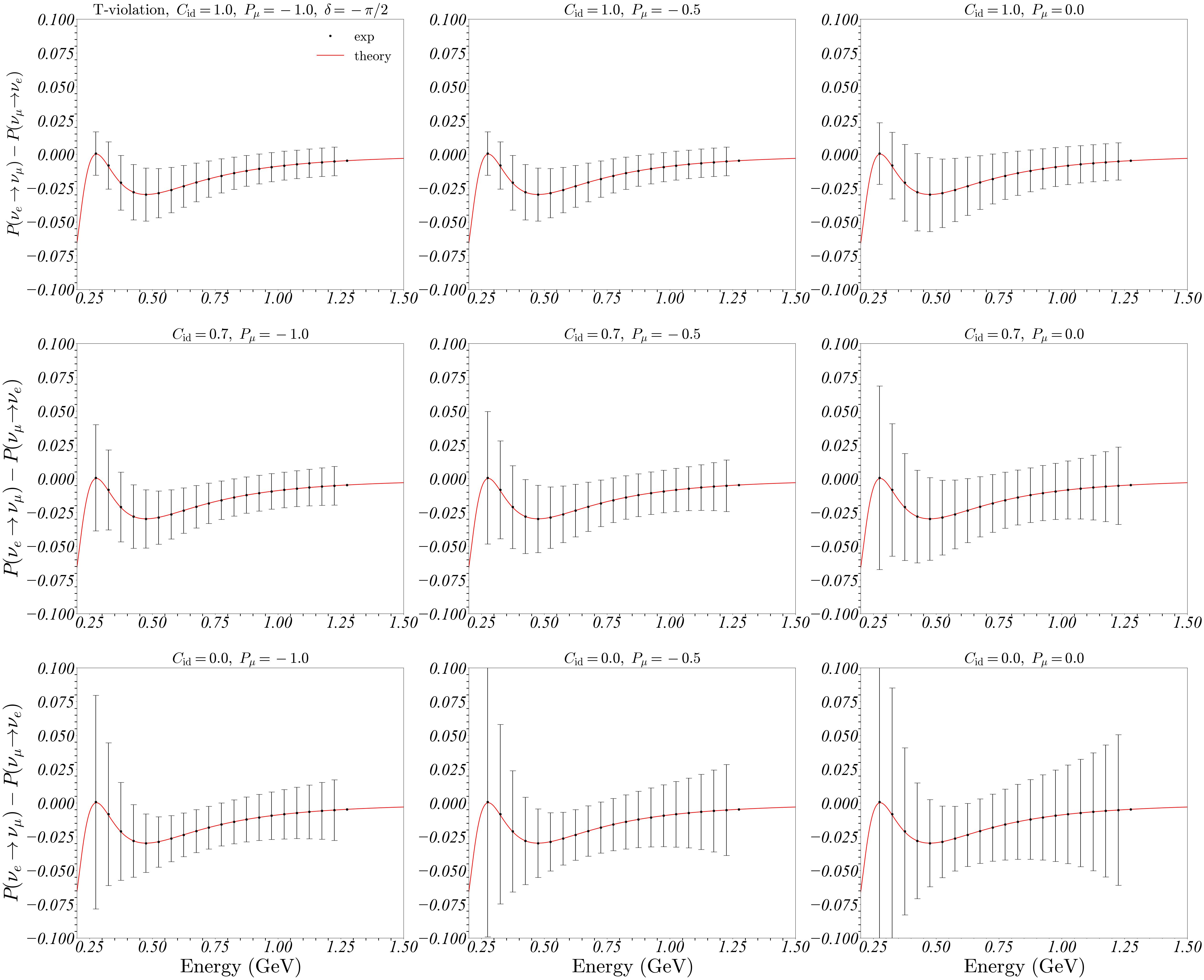
Figure 5: Reconstructed T violation from the expected neutrino flux with errors. The CP phase $\delta$ is set to be $-\pi/2$. From top to bottom, the graphs show the cases with the charge identification $C_{\rm id}=1.0,\ 0.7$, and $0.0$, and from left to right, show the cases with the anti-muon polarization $P_{\mu}=-1.0,\ -0.5$, and $0.0$.

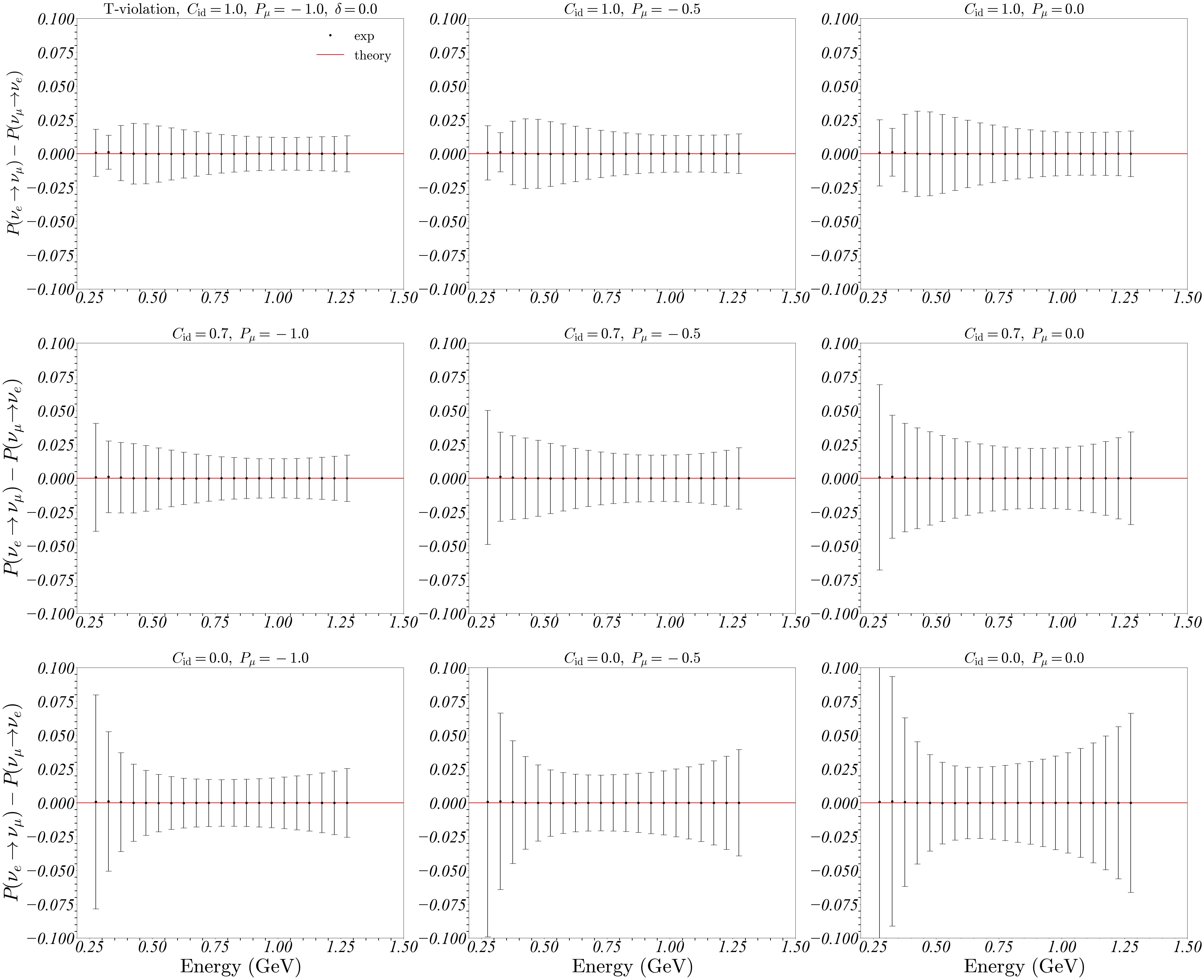
Figure 6: Reconstructed T violation from the expected neutrino flux with errors.The CP phase $\delta$ is set to be $0.0$.

One can see that the T violation is maximized near $E_{\nu}\sim 500$ MeV where the background is suppressed by the neutrino oscillation. This feature helps to give good sensitivity to T violation. Also, even for zero efficiency of the charge identification, $C_{\rm id}=0.0$, the sensitivity is not much worse than the case of the perfect identification $C_{\rm id}=1.0$ as we will see more explicitly later.

3.4 Parameter determination

In Fig. 7, we show the contour plots of $\chi^{2}_{\rm TV}(\delta^{\rm test},\rho^{\rm test})$. The shaded regions correspond to $1\sigma$, $2\sigma$, and $3\sigma$ allowed regions. We set true values as $\delta_{0}=-\pi/2$ and $\rho_{0}=2.6\ \mathrm{g/cm^{3}}$. Again, we take $P_{\mu}=-1.0$, $-0.5$, and $0.0$ from left to right, and $C_{\rm id}=1.0$, $0.7$, and $0.0$ from top to bottom. The results are almost unchanged for different choices of $C_{\rm id}$. This is quite important since the T-violation measurement can be performed without having a good identification strategy between $\nu_{\mu}$ and $\bar{\nu}_{\mu}$. Independent of $C_{\rm id}$, CP (or T) conserving point, $\delta=0$ and $\pi$ can be excluded at the level of 3$\sigma$ even for the unpolarized muon beam. For the best case, $C_{\rm id}=1.0$ and $P_{\mu}=-1.0$, the CP angle $\delta$ is determined with an accuracy of about $\pm$$$.

It is clear from the figure that $\chi^{2}_{\rm TV}$ depend on $\rho^{\rm test}$ only very slightly. This behavior is the obvious consequence of the time reversal symmetry of the earth. As we know that $\chi^{2}_{\rm TV}$ only depends on one of the parameters, $\delta$, we define the confidence level as that for a single degree of freedom, i.e., $\chi^{2}=1$ as 1$\sigma$. For completeness, we show in Fig. 8 the values of $\chi^{2}_{\rm TV}$ near the minima for choices of $\rho^{\rm test}$ as $0.0$ g/cm³, $2.6$ g/cm³, $3.6$ g/cm³, and $6.25$ g/cm³ while fixing the true value to be $\rho_{0}=2.6$ g/cm³.

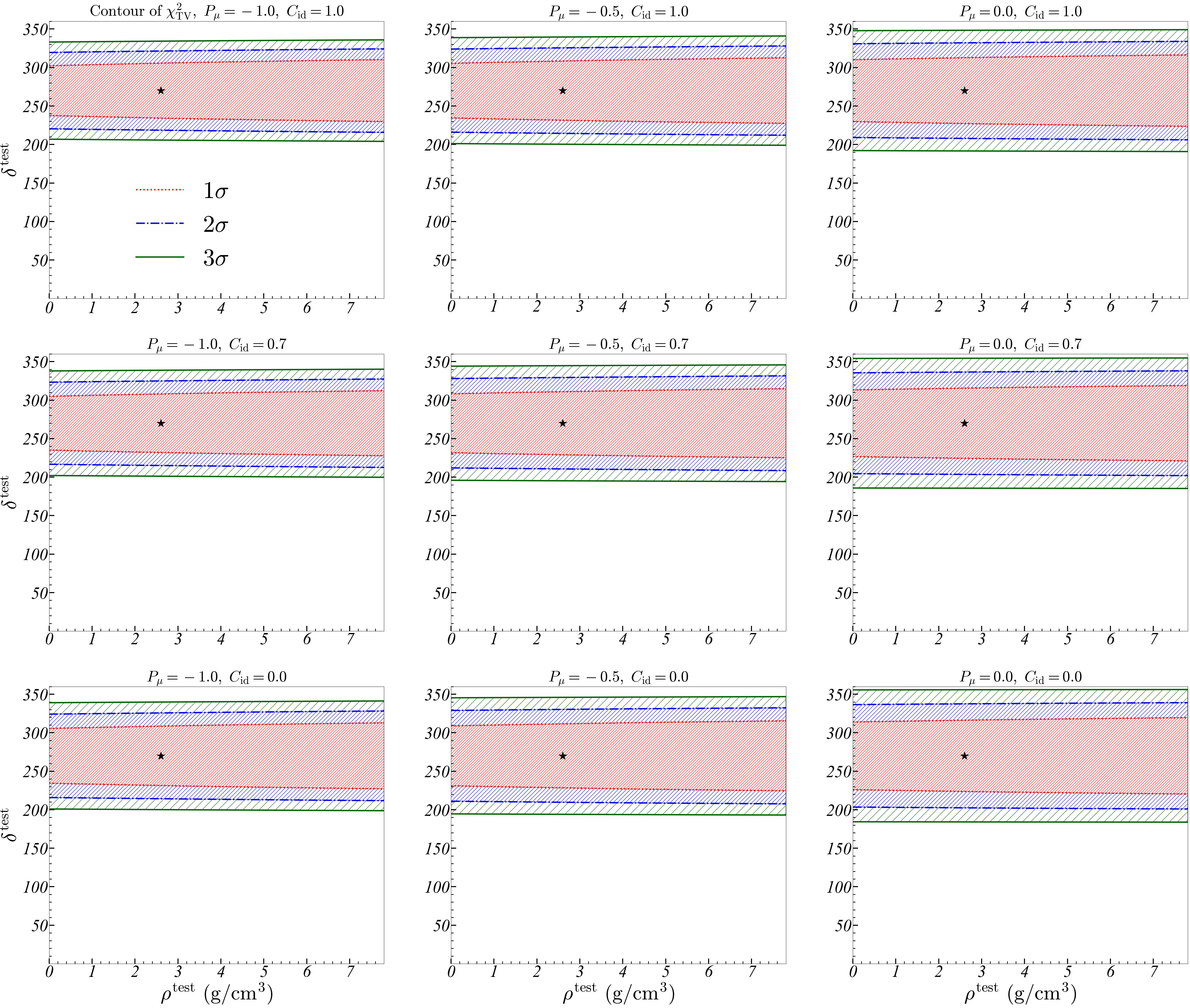
Figure 7: The contour of $\chi^{2}_{\rm TV}$ is defined in Eq. (14). The shaded regions represent $1\sigma$, $2\sigma$, and $3\sigma$ confidence interval, respectively, from inside to outside. From top to bottom, the figures show the cases with $C_{\rm id}=1.0,\ 0.7,\ 0.0$. From left to right, the figures show the cases with the anti-muon polarization $P_{\mu}=-1.0,\ -0.5,\ 0.0$. The stars in these figures represent the true input value ($\delta_{0}=-\pi/2,\ \rho_{0}=2.6\ \mathrm{g/cm^{3}}$).

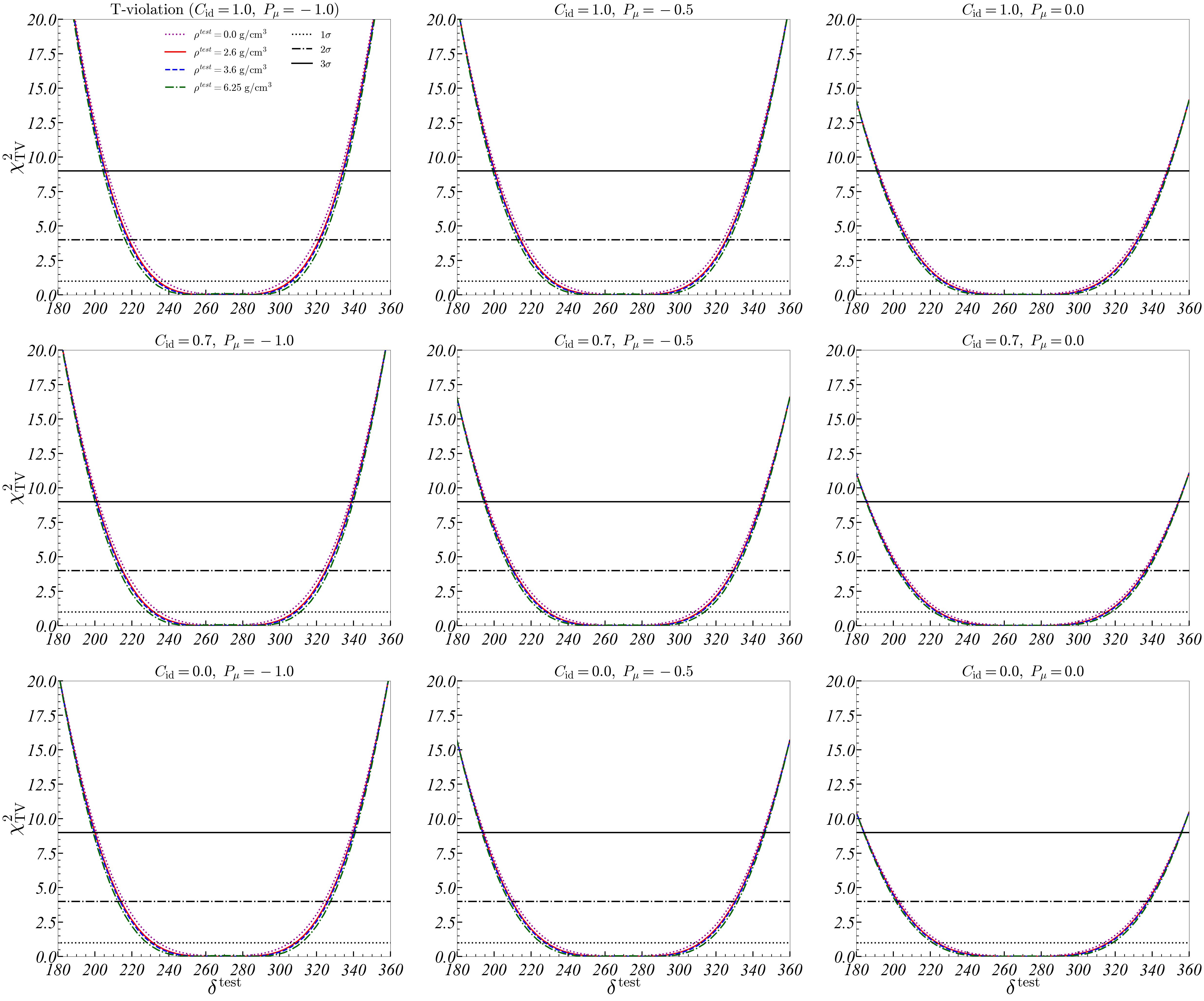
Figure 8: The values of $\chi^{2}_{\rm TV}$ in the region near $\delta=-\pi/2$. The purple dotted, red solid, blue dashed, and green dashdot lines represent $0.0~{}\mathrm{g/cm^{3}}$, $2.6~{}\mathrm{g/cm^{3}}$, $3.6~{}\mathrm{g/cm^{3}}$, and $6.25~{}\mathrm{g/cm^{3}}$, respectively. From top to bottom, the figures show the cases with $C_{\rm id}=1.0,\ 0.7,\ 0.0$. From left to right, the figures show the cases with anti-muon polarization $P_{\mu}=-1.0,\ -0.5,\ 0.0$. Three horizontal lines ($1\sigma$ dot, $2\sigma$ dashdot, $3\sigma$) are values of $\chi^{2}$ for 1 d.o.f. The true input values are set to be $\delta_{0}=-\pi/2$ and $\rho_{0}=2.6\ \mathrm{g/cm^{3}}$.

3.5 $\chi^{2}$ analysis of CP violation at T2HK

In contrast to the T-violation measurement, CP violation suffers from the uncertainties in the matter profile of the earth. We consider CP violation,

$$P^{\rm CP}_{j}=P_{j}(\nu_{\mu}\to\nu_{e})\big{|}_{\rm T2HK}-P_{j}(\bar{\nu}_{\mu}\to\bar{\nu}_{e})\big{|}_{\rm T2HK},$$ (16)

and we define $\chi^{2}_{\rm CP}(\delta^{\rm test},\rho^{\rm test})$ in a similar way as T violation. We show the contour of the confidence interval in Fig. 9.

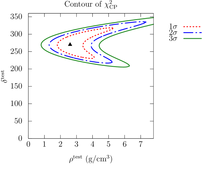
Figure 9: The contour of $\chi^{2}_{\rm CP}$. The red dot, blue dashdot, and green solid lines represent $1\sigma$, $2\sigma$, and $3\sigma$ confidence interval, respectively. The triangle symbol represent the true input value ($\delta_{0}=-\pi/2,\ \rho_{0}=2.6\ \mathrm{g/cm^{3}}$).

We see a non-trivial dependence of the allowed region on $\rho^{\rm test}$, and it is clear that a good knowledge of the matter density profile will be necessary for this measurement. The measurement of T violation will be an important additional information for the measurement of the CP angle $\delta$.

3.6 Discussion: possible CPT test?

Although we do not try in this paper, one would be able to perform a similar analysis for CPT violation,

$$P_{j}^{\rm CPT}=P_{j}(\nu_{e}\to\nu_{\mu})-P_{j}(\bar{\nu}_{\mu}\to\bar{\nu}_{e})\big{|}_{\rm T2HK}=P_{j}^{\rm TV}+P_{j}^{\rm CP}.$$ (17)

Under our assumptions, this quantity would not measure anything as it should be trivially vanishing up to matter effects. Nevertheless, this will provide us with a quite important test of our underlying assumptions such as the three-neutrino scheme as well as quantum field theory.

Indeed, the neutrino mass is the smallest mass scale of the Standard Model, and its nature is totally unknown. Among many scenarios, there have been proposals of explaining the neutrino masses via small violation of the Lorentz invariance, for example, in Refs. [29, 30]. The analysis of this kind will be a quite important fundamental test of symmetry in physical laws of the Universe.

4 Summary

Motivated by the recent discussions of the intense muon beam for muon colliders, we studied the possibility of measuring T violation, $P(\nu_{e}\to\nu_{\mu})-P(\nu_{\mu}-\nu_{e})$ by assuming the baseline from J-PARC to Hyper-Kamiokande. We take a scenario that a $\mu^{+}$ beam will be available at J-PARC as proposed in Ref. [15], so that a large flux of $\nu_{e}$ will be pointing towards Hyper-Kamiokande. By combining with the measurement at the T2HK experiment which uses the conventional $\nu_{\mu}$ beam, the T violation can be defined. The T violation, the probability difference above, is a quantity that does not suffer from the uncertainty of matter density of the earth.

Under reasonable assumptions on the muon intensity, the results show that the observation of T violation is possible if $|\sin\delta|$ is large enough. For the case of maximum CP violation, i.e., $\delta=-\pi/2$, one can exclude the CP invariant theory $\delta=0$ or $\pi$ at more than $3\sigma$ level. There are two important parameters in the experimental set-up, which are the beam polarization of muons and the efficiency of the charge identification to distinguish $\nu_{\mu}$ from $\bar{\nu}_{\mu}$ at Hyper-Kamiokande. There is a fortunate fact that the background $\bar{\nu}_{\mu}$ events from the muon decays are suppressed at the most important energy range for T violation by setting the muon beam energy to give the oscillation maximum. Even with no ability of distinguish $\nu_{\mu}$ and $\bar{\nu}_{\mu}$ events, the sensitivities do not change significantly. Rather, the beam polarization to increase the forward $\nu_{e}$ will be more important at the actual experiment.

We considered $\chi^{2}$ for CP violation and compared it with that for T violation. For CP violation, $\chi^{2}_{\rm CP}$ depends significantly on both $\delta$ and $\rho$, whereas for T violation, $\chi^{2}_{\rm TV}$ is almost independent on $\rho$. This means T violation would not suffer from the uncertainties in the matter density profile of the earth, and give a clearer signal.

Testing T violation in the lepton sector has not been conducted yet, so it remains as an important task in particle physics. In this study, we demonstrated the feasibility for the measurement, while we considered only the statistical error. A more complete analysis will be necessary to establish the feasibility. Once it is measured, it is going to be a very nontrivial test of the three neutrino paradigm or possibly of the CPT theorem which is one of the most fundamental features in the quantum field theory.

References

- [1] T2K, K. Abe et al., “Improved constraints on neutrino mixing from the T2K experiment with protons on target,” Phys. Rev. D 103 no. 11, (2021) 112008, arXiv:2101.03779 [hep-ex].
- [2] NOvA, M. A. Acero et al., “Improved measurement of neutrino oscillation parameters by the NOvA experiment,” Phys. Rev. D 106 no. 3, (2022) 032004, arXiv:2108.08219 [hep-ex].
- [3] Hyper-Kamiokande, K. Abe et al., “Hyper-Kamiokande Design Report,” arXiv:1805.04163 [physics.ins-det].
- [4] JUNO, F. An et al., “Neutrino Physics with JUNO,” J. Phys. G 43 no. 3, (2016) 030401, arXiv:1507.05613 [physics.ins-det].
- [5] DUNE, R. Acciarri et al., “Long-Baseline Neutrino Facility (LBNF) and Deep Underground Neutrino Experiment (DUNE): Conceptual Design Report, Volume 2: The Physics Program for DUNE at LBNF,” arXiv:1512.06148 [physics.ins-det].
- [6] K2K, M. H. Ahn et al., “Measurement of Neutrino Oscillation by the K2K Experiment,” Phys. Rev. D 74 (2006) 072003, arXiv:hep-ex/0606032.
- [7] J. Arafune and J. Sato, “CP and T violation test in neutrino oscillation,” Phys. Rev. D 55 (1997) 1653–1658, arXiv:hep-ph/9607437.
- [8] J. Arafune, M. Koike, and J. Sato, “CP violation and matter effect in long baseline neutrino oscillation experiments,” Phys. Rev. D 56 (1997) 3093–3099, arXiv:hep-ph/9703351. [Erratum: Phys.Rev.D 60, 119905 (1999)].
- [9] M. Koike and J. Sato, “T violation search with very long baseline neutrino oscillation experiments,” Phys. Rev. D 62 (2000) 073006, arXiv:hep-ph/9911258.
- [10] M. Koike, T. Ota, and J. Sato, “Ambiguities of theoretical parameters and CP/T violation in neutrino factories,” Phys. Rev. D 65 (2002) 053015, arXiv:hep-ph/0011387.
- [11] J. Pinney and O. Yasuda, “Correlations of errors in measurements of CP violation at neutrino factories,” Phys. Rev. D 64 (2001) 093008, arXiv:hep-ph/0105087.
- [12] S. Geer, “Neutrino beams from muon storage rings: Characteristics and physics potential,” Phys. Rev. D 57 (1998) 6989–6997, arXiv:hep-ph/9712290. [Erratum: Phys.Rev.D 59, 039903 (1999)].
- [13] MAP, D. M. Kaplan, “A Staged Muon-Based Neutrino and Collider Physics Program,” in CERN Council Open Symposium on European Strategy for Particle Physics. 7, 2012. arXiv:1212.4214 [physics.acc-ph].
- [14] Y. Kondo, “Re-Acceleration of Ultra Cold Muon in J-PARC Muon Facility,” 9th International Particle Accelerator Conference 6 (2018) .
- [15] Y. Hamada, R. Kitano, R. Matsudo, H. Takaura, and M. Yoshida, “TRISTAN,” PTEP 2022 no. 5, (2022) 053B02, arXiv:2201.06664 [hep-ph].
- [16] M. Abe et al., “A New Approach for Measuring the Muon Anomalous Magnetic Moment and Electric Dipole Moment,” PTEP 2019 no. 5, (2019) 053C02, arXiv:1901.03047 [physics.ins-det].
- [17] A. M. Dziewonski and D. L. Anderson, “Preliminary reference earth model,” Phys. Earth Planet. Interiors 25 (1981) 297–356.
- [18] P. F. Harrison and W. G. Scott, “CP and T violation in neutrino oscillations and invariance of Jarlskog’s determinant to matter effects,” Phys. Lett. B 476 (2000) 349–355, arXiv:hep-ph/9912435.
- [19] V. A. Naumov, “Three neutrino oscillations in matter and topological phases,” Sov. Phys. JETP 74 (1992) 1–8.
- [20] V. A. Naumov, “Three neutrino oscillations in matter, CP violation and topological phases,” Int. J. Mod. Phys. D 1 (1992) 379–399.
- [21] C. Jarlskog, “A Basis Independent Formulation of the Connection Between Quark Mass Matrices, CP Violation and Experiment,” Z. Phys. C 29 (1985) 491–497.
- [22] C. Jarlskog, “Commutator of the Quark Mass Matrices in the Standard Electroweak Model and a Measure of Maximal CP Nonconservation,” Phys. Rev. Lett. 55 (1985) 1039.
- [23] V. D. Barger, S. Geer, and K. Whisnant, “Long baseline neutrino physics with a muon storage ring neutrino source,” Phys. Rev. D 61 (2000) 053004, arXiv:hep-ph/9906487.
- [24] J. F. Beacom and M. R. Vagins, “GADZOOKS! Anti-neutrino spectroscopy with large water Cherenkov detectors,” Phys. Rev. Lett. 93 (2004) 171101, arXiv:hep-ph/0309300.
- [25] Super-Kamiokande, M. Harada et al., “Search for Astrophysical Electron Antineutrinos in Super-Kamiokande with 0.01% Gadolinium-loaded Water,” Astrophys. J. Lett. 951 no. 2, (2023) L27, arXiv:2305.05135 [astro-ph.HE].
- [26] R. Akutsu, “A Study of Neutrons Associated with Neutrino and Antineutrino Interactions on the Water Target at the T2K Far Detector,” Ph.D. thesis, University of Tokyo (2019) .
- [27] J. A. Formaggio and G. P. Zeller, “From eV to EeV: Neutrino Cross Sections Across Energy Scales,” Rev. Mod. Phys. 84 (2012) 1307–1341, arXiv:1305.7513 [hep-ex].
- [28] Particle Data Group, R. L. Workman et al., “Review of Particle Physics,” PTEP 2022 (2022) 083C01.
- [29] S. R. Coleman and S. L. Glashow, “High-energy tests of Lorentz invariance,” Phys. Rev. D 59 (1999) 116008, arXiv:hep-ph/9812418.
- [30] A. G. Cohen and S. L. Glashow, “Very special relativity,” Phys. Rev. Lett. 97 (2006) 021601, arXiv:hep-ph/0601236.