Pattern formation by advection-diffusion
in new economic geography

Abstract

A new economic geography model is proposed in which the migration of mobile workers is proximate and perturbed by non-economic factors. The model consists of a tractable core-periphery model assuming a quasi-linear log utility function of consumers and an advection-diffusion equation governing the time evolution of a population distribution. The stability of a spatially homogeneous stationary solution and the large time behavior of solutions to the model on a one-dimensional periodic space are investigated. When the spatially homogeneous stationary solution is unstable, solutions starting around it are found to eventually form spatial patterns with several urban areas in which mobile workers agglomerate.

Keywords:  advection-diffusion; core-periphery model; economic agglomeration; new economic geography; partial differential equation; pattern formation; self-organization; transport costs

JEL classification: R12, R40, C62, C63, C68

1 Introduction

In basic models of new economic geography (NEG), the replicator dynamics of population is often employed. That is, for a geographic space denoted by $\Omega$, the time evolution of a population distribution $\lambda$ on $\Omega$ is assumed to be

$$\frac{\partial\lambda}{\partial t}(t,x)=v\left[\omega(t,x)-\tilde{\omega}(t)\right]\lambda(t,x),\hskip 8.53581ptv>0$$ (1)

for time $t\geq 0$ and $x\in\Omega$. Here, $\omega$ and $\tilde{\omega}$ stand for real wages, and a spatially average realwage, respectively. The equation (1) states that the population migrates from where real wages are below average to where they are above average. In this formulation, it is assumed that the population can perceive the global spatial distribution of real wages and can migrate without any barriers, no matter how great the distance.

However, there are obviously cases where this may not be appropriate in the real world. We know that population often migrates only proximally, and migration would be subject to random perturbations due to non-economic factors. Based on this idea, Mossay (2003) has proposed a pioneering model in which the migration process of population is expressed by the partial differential equation

$$\frac{\partial\lambda}{\partial t}(t,x)+\frac{\partial}{\partial x}\left(\lambda(t,x)\frac{\partial\omega}{\partial x}(t,x)\right)=d\frac{\partial^{2}\lambda}{\partial x^{2}}(t,x),\hskip 8.53581ptd>0$$ (2)

in one-dimensional periodic space. The stability of a spatially homogeneous stationary solution to the model has been discussed in Mossay (2003). Then, the next natural question is what spatial patterns emerge from such a partial differential equation model. However, obtaining a time-evolving solution to this model is difficult. Specifically, since the Mossay model is based on the original Core-Periphery (CP) model proposed by Krugman (1991), one must solve a nonlinear fixed point problem for the population distribution $\lambda$ at each time $t\geq 0$ to obtain a market equilibrium solution for computing the realwage $\omega$. This may lead to difficulties in elucidating the behavior of time-evolving solutions of the Mossay model, even numerically.

In this paper, instaed of the CP model by Krugman (1991), we use a more computationally tractable model which is originally devised by Pflüger (2004) and extended to one on a continuous space by Ohtake (2023a) to avoid difficulties in computing market equilibrium solutions. It is found that if a spatially homogeneous stationary solution is unstable, then a solution starting around it eventually forms several urban areas in which population agglomerates. In the case that the spatially homogenous stationary solution is unstable, the number of the urban areas tends to decrease with decreasing transport costs or with increasing preference for variety.

2 The model

2.1 Settings

The economy consists of two sectors: manufacturing and agriculture. The manufacturing is under monopolistic competition and the agriculture is under perfect competition. In the manufacturing, one firm produces one variety of an infinite number of varieties of differentiated goods. In the agriculture, a single variety of goods are produced. When goods are transported between regions, the manufactured goods incur transport costs but the agricultural goods do not. For the transport costs, the so-called iceberg transport technology is assumed. That is, goods melt away during transportation, depending on the distance over which they are transported. There are two types of workers: mobile workers who can migrate through space and immobile workers who cannot. In the manufacturing sector, the mobile workers are used as a fixed input and the immobile workers as a marginal input. In the agricultural sector, one unit of goods is produced by one unit of the immobile workers.

2.2 Model equations

We handle the following system of integral-differential equations

$$\left\{\begin{aligned} &G(t,x)=\left[\frac{1}{F}\int_{\Omega}\lambda(t,y)T(x,y)^{1-\sigma}dy\right]^{\frac{1}{1-\sigma}},\\ &w(t,x)=\frac{\mu}{\sigma F}\int_{\Omega}\left(\phi(y)+\lambda(t,y)\right)G(t,y)^{\sigma-1}T(x,y)^{1-\sigma}dy,\\ &\omega(t,x)=w(t,x)-\mu\ln G(t,x),\\ &\frac{\partial\lambda}{\partial t}(t,x)+a\nabla\cdot\left(\lambda(t,x)\nabla\omega(t,x)\right)=d\Delta\lambda(t,x)\end{aligned}\right.$$ (3)

for $(t,x)\in[0,\infty)\times\Omega$ with an initial condition $\lambda(0,x)=\lambda_{0}(x)$. Here, $\Omega$ is a bounded subset in the $n$-dimensional Euclidean space with $n\geq 1$. The given function $\phi\geq 0$ which satisfies

$$\int_{\Omega}\phi(x)dx=\Phi>0$$

denotes the population density of immobile workers. The unknown function $\lambda\geq 0$ which satisfies

$$\int_{\Omega}\lambda(t,x)dx=\Lambda>0,~{}\forall t\geq 0$$ (4)

denotes the population density of mobile workers. Other unknown functions $w$, $G$, and $\omega$ denote the nominal wage of mobile workers, the price index of manufactured goods, and the real wage of mobile workers, respectively. The iceberg transport technology is expressed by the two-variable function $T$, that is, $T(x,y)\geq 1$ units of a variety of manufactured goods must be shipped to deliver one unit of the variety from $x\in\Omega$ to $y\in\Omega$.

The model equation consists of the first three equations giving a market equilibrium and the fourth equation describing the migration of mobile workers. The second term on the left-hand side of the fourth equation describes the migration along a real wage gradient, i.e., advection, and the right-hand side of the equation describes the random movement of mobile workers independent of the gradient, i.e., diffusion. See Appendix (Subsection 6.1) for the derivation of this advection-dissusion equation.

The parameters included in the model are as follows. The degree to which each consumer favors manufactured goods is $\mu\in[0,1)$. The elasticity of substitution between any two varieties of manufactured goods is $\sigma>1$. The closer $\sigma$ is to $1$, the stronger the preference for variety of consumers is. The size of the fixed input for the production of manufactured goods is $F>0$. The strength of advection and diffusion are expressed by the advection coefficient $a\geq 0$ and the diffusion coefficient $d\geq 0$, respectively.

2.3 Racetrack economy

In the following, we consider a so-called racetrack economy, that is, a model on the one-dimensional circumference of radius $\rho>0$ denoted by $S$. For this purpose, we consider the model (3) with the periodic boundary condition on the interval $[-\rho\pi,\rho\pi]\subset\mathbb{R}$, and a point $x\in S$ is identified with a real number $x\in[-\rho\pi,\rho\pi]$. Therefore, the integration of a periodic function $h$ over $S$ is calculated by

$$\int_{S}h(x)dx=\int_{-\rho\pi}^{\rho\pi}h(x)dx$$

By transforming the variable by

$$x=\rho r$$ (5)

with an angle $r\in[-\pi,\pi]$, we see that

$$\int_{S}h(x)dx=\int_{-\pi}^{\pi}h(\rho r)\rho dr.$$ (6)

The fourth equation in (3) is then

$$\frac{\partial\lambda}{\partial t}(t,\rho r)+\frac{a}{\rho^{2}}\frac{\partial}{\partial r}\left(\lambda(t,\rho r)\frac{\partial\omega}{\partial r}(t,\rho r)\right)=\frac{d}{\rho^{2}}\frac{\partial^{2}\lambda}{\partial r^{2}}(t,\rho r).$$ (7)

We specify a function representing the iceberg transport cost as

$$T(x,y)=e^{\tau D(x,y)}$$ (8)

with $\tau\geq 0$. Here, $D(x,y)$ stands for the shorter distance between $x\in S$ and $y\in S$ along $S$. If $x=\rho r$ and $y=\rho s$ with $r\in[-\pi,\pi]$ and $s\in[-\pi,\pi]$, then

$$D\left(x,y\right)(=D\left(\rho r,\rho s\right))=\rho\min\left\{|r-s|,2\pi-|r-s|\right\}.$$

Then, it is convinient to define a constant $\alpha$ as

$$\alpha:=(\sigma-1)\tau.$$ (9)

Thus, the racetrack economy we consider is

$$\left\{\begin{aligned} &G(t,\rho r)=\left[\frac{1}{F}\int_{-\pi}^{\pi}\lambda(t,\rho s)e^{-\alpha D(\rho r,\rho s)}\rho ds\right]^{\frac{1}{1-\sigma}},\\ &w(t,\rho r)=\frac{\mu}{\sigma F}\int_{-\pi}^{\pi}\left(\phi(\rho s)+\lambda(t,\rho s)\right)G(t,\rho s)^{\sigma-1}e^{-\alpha D(\rho r,\rho s)}\rho ds,\\ &\omega(t,\rho r)=w(t,\rho r)-\mu\ln G(t,\rho r),\\ &\frac{\partial\lambda}{\partial t}(t,\rho r)+\frac{a}{\rho^{2}}\frac{\partial}{\partial r}\left(\lambda(t,\rho r)\frac{\partial\omega}{\partial r}(t,\rho r)\right)=\frac{d}{\rho^{2}}\frac{\partial^{2}\lambda}{\partial{r}^{2}}(t,\rho r)\end{aligned}\right.$$ (10)

for $(t,r)\in[0,\infty)\times[-\pi,\pi]$ with an initial condition $\lambda(0,\rho r)=\lambda_{0}(\rho r)$.

3 Stationary solution

3.1 Homogeneous stationary solution

We consider a homogeneous stationary solution where the mobile and immobile populations are uniformly distributed on $S$. Same as Ohtake (2023a), by substituting the homogeneous population density of immobile workers $\overline{\phi}$ and that of mobile workers $\overline{\lambda}$

$$\overline{\phi}=\frac{\Phi}{2\pi\rho},$$ (11)

$$\overline{\lambda}=\frac{\Lambda}{2\pi\rho}$$ (12)

into the first and second equations of (10), we have a homogeneous nominal wage $\overline{w}$ and price index $\overline{G}$ as

$$\overline{w}=\frac{\mu\left(\overline{\phi}+\overline{\lambda}\right)}{\sigma\overline{\lambda}},$$ (13)

$$\overline{G}=\left[\frac{2\overline{\lambda}\left(1-e^{-\alpha\rho\pi}\right)}{F\alpha}\right]^{\frac{1}{1-\sigma}},$$ (14)

respectively. Then, from the third equation of (3), it is obvious that the real wage is also homogeneous as

$$\overline{\omega}=\overline{w}-\mu\ln\overline{G}.$$ (15)

3.2 Stability of the stationary solution

3.2.1 Linearized equations

Let $\varDelta\lambda$, $\varDelta w$, $\varDelta G$, and $\varDelta\omega$ be small perturbations added to the homogeneous stationary states (12), (13), (14), and (15), respectively. Note that

$$\int_{S}\varDelta\lambda(t,x)dx=0,~{}\forall t\geq 0$$ (16)

must hold because of (4). Substituting $\lambda=\overline{\lambda}+\varDelta\lambda$, $w=\overline{w}+\varDelta w$, $G=\overline{G}+\varDelta G$, and $\omega=\overline{\omega}+\varDelta\omega$ into (10) , and leaving only the first-order terms with respect to the small perturbations, we obtain the following linearized equations.

$$\left\{\begin{aligned} &\varDelta w(t,\rho r)\\ &=\frac{\mu(\sigma-1)(\overline{\phi}+\overline{\lambda})\overline{G}^{\sigma-2}}{F\sigma}\int_{-\pi}^{\pi}\varDelta G(t,\rho s)e^{-\alpha D(\rho r,\rho s)}\rho ds\\ &\hskip 71.13188pt+\frac{\mu\overline{G}^{\sigma-1}}{F\sigma}\int_{-\pi}^{\pi}\varDelta\lambda(t,\rho s)e^{-\alpha D(\rho r,\rho s)}\rho ds,\\ &\varDelta G(t,\rho r)=-\frac{\overline{G}^{\sigma}}{(\sigma-1)F}\int_{-\pi}^{\pi}\varDelta\lambda(t,\rho s)e^{-\alpha D(\rho r,\rho s)}\rho ds,\\ &\varDelta\omega(t,\rho r)=\varDelta w(t,\rho r)-\frac{\mu}{\overline{G}}\varDelta G(t,\rho r),\\ &\frac{\partial\varDelta\lambda}{\partial t}(t,\rho r)+\frac{a\overline{\lambda}}{\rho^{2}}\frac{\partial^{2}\varDelta\omega}{{\partial r}^{2}}(t,\rho r)=\frac{d}{\rho^{2}}\frac{\partial^{2}\varDelta\lambda}{{\partial r}^{2}}(t,\rho r)\end{aligned}\right.$$ (17)

for $[0,\infty)\times[-\pi,\pi]$. Let us define the Fourier series of a small perturbation $\varDelta h$ by

$$\varDelta h(t,\rho r)=\frac{1}{2\pi}\sum_{k=0,\pm 1,\pm 2,\cdots}\hat{h}_{k}(t)e^{ikr},$$ (18)

where the Fourier coefficient is defined by

$$\hat{h}_{k}(t)=\int_{-\pi}^{\pi}\varDelta h(t,\rho r)e^{-ikr}dr.$$

In (18), we refer to $k$ and $e^{ikr}$ as a spatial frequency and a $k$-th mode, respectively. By expanding the small perturbations of equations (17) into the Fourier series, we obtain the equations for the Fourier coefficients

$$\left\{\begin{aligned} &\hat{w}_{k}=\frac{\mu(\sigma-1)(\overline{\phi}+\overline{\lambda})}{\sigma\overline{\lambda}\overline{G}}Z_{k}\hat{G}_{k}+\frac{\mu}{\sigma\overline{\lambda}}Z_{k}\hat{\lambda}_{k},\\ &\hat{G}_{k}=-\frac{\overline{G}}{(\sigma-1)\overline{\lambda}}Z_{k}\hat{\lambda}_{k},\\ &\hat{\omega}_{k}=\hat{w}_{k}-\frac{\mu}{\overline{G}}\hat{G}_{k},\\ &\frac{d\hat{\lambda}_{k}}{dt}-\frac{a\overline{\lambda}k^{2}}{\rho^{2}}\hat{\omega}_{k}=-\frac{dk^{2}}{\rho^{2}}\hat{\lambda}_{k}\end{aligned}\right.$$ (19)

for each $k=\pm 1,\pm 2,\cdots$. We do not have to consider the case $k=0$ because $\hat{\lambda}_{0}=0$ due to (16). The variable $Z_{k}$ in (19) is defined by

$$Z_{k}:=\frac{\alpha^{2}\rho^{2}\left(1-(-1)^{k}e^{-\alpha\rho\pi}\right)}{\left(k^{2}+\alpha^{2}\rho^{2}\right)\left(1-e^{-\alpha\rho\pi}\right)}.$$

It is known that $Z_{k}$ is monotonically increasing with respect to $\alpha\rho\geq 0$ and $\lim_{\alpha\rho\to 0}Z_{k}=0$ and $\lim_{\alpha\rho\to\infty}Z_{k}=1$ hold. By solving (19), we have

$$\frac{d\hat{\lambda}_{k}}{dt}=\Gamma_{k}\hat{\lambda}_{k},$$ (20)

where

$$\Gamma_{k}:=\frac{k^{2}}{\rho^{2}}\left[a\mu Z_{k}\left(-\frac{\overline{\phi}+\overline{\lambda}}{\sigma\overline{\lambda}}Z_{k}+\frac{2\sigma-1}{\sigma(\sigma-1)}\right)-d\right]$$ (21)

It is easy toverify that $\Gamma_{k}=\Gamma_{-k}$ from $Z_{k}=Z_{-k}$. From (20), if $\Gamma_{k}<0$, then the amplitude of the $k$-th mode decays to $0$ with time, and let us call the mode a stabilized mode. Meanwhile, if $\Gamma_{k}>0$, then the amplitude of the $k$-th mode grows with time, and let us call the mode a destabilized mode. It is easy from (21) to see that if the diffusion coefficient $d>0$ is sufficiently large, then the $k$-th mode becomes stabilized. This is intuitive because diffusion must oppose agglomeration.

Figure 1 shows how $\Gamma_{k}$ depends on the control parameters $\tau$ and $\sigma$. Other parameters are fixed to $\mu=0.6$, $a=0.5$, $d=0.005$, $F=1$, $\Lambda=1$, $\Phi=10$, and $\rho=1$. Subfigure 1(a) describes $\Gamma_{k}$ as a function of $\tau$ under $\sigma=5$ for frequencies $k=1,2,\cdots,5$. For each $k$, there exist two critical points $\tau_{1}<\tau_{2}$ at which $\Gamma_{k}=0$. For $\tau\in(\tau_{1},\tau_{2})$, $\Gamma_{k}>0$. For $\tau\in(0,\tau_{1})$ and $\tau\in(\tau_{2},\infty)$, $\Gamma_{k}<0$. Subfigure 1(b) describes $\Gamma_{k}$ as a function of $\sigma$ under $\tau=0.5$ for frequencies $k=1,2,\cdots,5$. For each $k$, except for $k=1$ and $3$, there exist two critical points $\sigma_{1}<\sigma_{2}$ at which $\Gamma_{k}=0$. For $\sigma\in(\sigma_{1},\sigma_{2})$, $\Gamma_{k}>0$. For $\sigma\in(0,\sigma_{1})$ and $\sigma\in(\sigma_{2},\infty)$, $\Gamma_{k}<0$. For $k=1$ and $3$, there only exists $\sigma_{2}$ such that $\Gamma_{k}>0$ for $\sigma\in(1,\sigma_{2})$ and $\Gamma_{k}<0$ for $\sigma\in(\sigma_{2},\infty)$.

In each case, the upper critical points ($\tau_{2}$ and $\sigma_{2}$) are the symmetry breaking points when each parameter becomes smaller. It can be seen that the values of the upper critical points increase as the absolute value of a frequency increases. This indicates that higher frequency modes, which have large $|k|$, get destabilized before lower frequency modes, which have small $|k|$, as the transport costs decrease or the preference for variety strengthens.

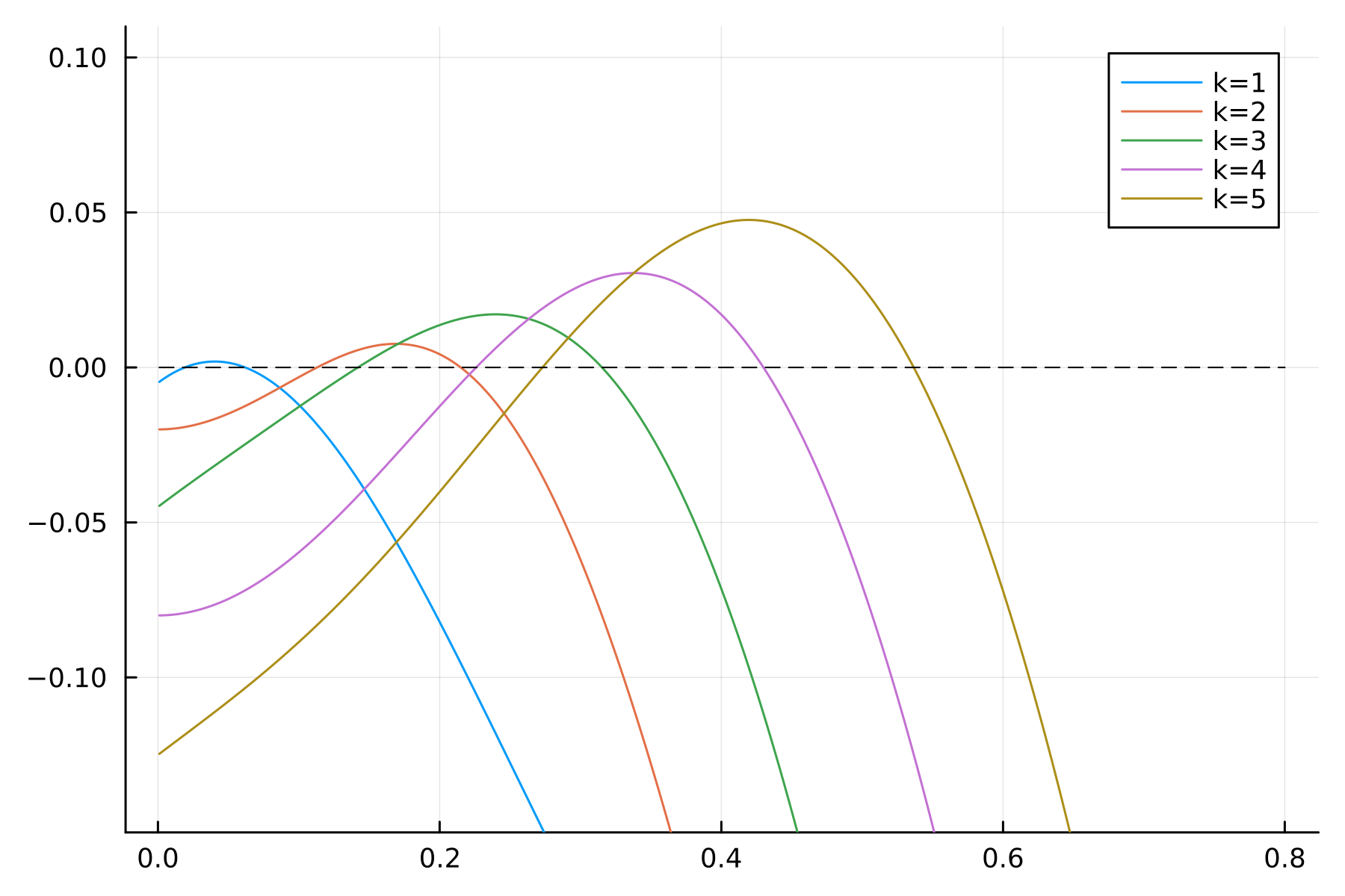
(a) $\Gamma_{k}$ as a function of $\tau$

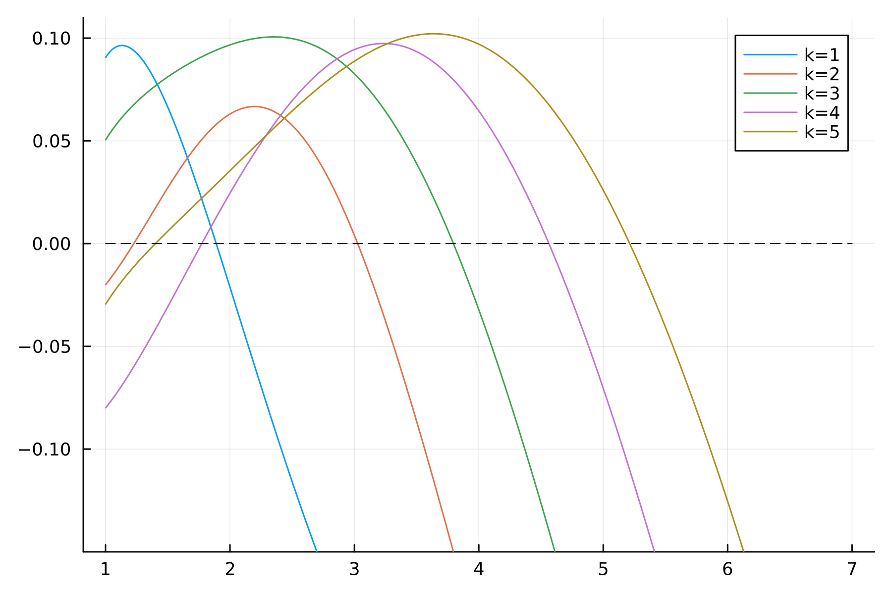
(b) $\Gamma_{k}$ as a function of $\sigma$

Figure 1: Graphs of $\Gamma_{k}$

4 Numerical simulations

4.1 Numerical scheme

The time variable $t\in[0,\infty)$ is discretized by a small fragment $\varDelta t$ as $t_{n}=n\varDelta t$ for $n=0,1,2,\cdots$. The space variable $r\in[-\pi,\pi)$ is descretized with $N$ equally spaced nodes denoted by $r_{i}=-\pi+(i-1)\varDelta r$ for $i=1,2,\cdots,N$ where $\varDelta r=2\pi/N$. A function $h$ on $[0,\infty)\times S$ is approximated by a vector $h^{n}=[h_{1}^{n},h_{2}^{n},\cdots,h_{N}^{n}]\in\mathbb{R}^{N}$ each of which element corresponds to an approximated value of $h(t_{n},\rho r_{i})$. We often have to mention elements such as $h_{N+1}^{n}$ and $h_{0}^{n}$. In that case, the periodicity naturally leads to $h_{N+1}^{n}:=h^{n}_{1}$ and $h_{0}^{n}:=h_{N}^{n}$. The integration of $h$ on $S$ is approximated as

$$\int_{-\pi}^{\pi}h(t_{n},\rho r)\rho dr\fallingdotseq\sum_{i=1}^{N}h_{i}^{n}\rho\varDelta r,$$

which is equivalent to the approximation by using the trapezoidal rule in the periodic condition.

By defining a flux $f$ as

$$f(t,\rho r):=\lambda(t,\rho r)\frac{\partial\omega}{\partial r}(t,\rho r),$$ (22)

we see that (7) becomes

$$\frac{\partial\lambda}{\partial t}(t,\rho r)+\frac{a}{\rho^{2}}\frac{\partial f}{\partial r}(t,\rho r)=\frac{d}{\rho^{2}}\frac{\partial^{2}\lambda}{\partial r^{2}}(t,\rho r).$$

We approximate the time derivative by the forward-difference method as

$$\frac{\partial\lambda}{\partial t}(t^{n},\rho r_{j})\fallingdotseq\frac{\lambda^{n+1}_{j}-\lambda^{n}_{j}}{\varDelta t}.$$ (23)

The diffusion term is approximated by the well-known formula

$$\frac{\partial^{2}\lambda}{\partial r^{2}}(t,\rho r)\fallingdotseq\frac{\lambda^{n}_{j+1}-2\lambda^{n}_{j}+\lambda^{n}_{j-1}}{\varDelta r^{2}}.$$ (24)

To approximate the second term on the left-hand side, we follow a finite-volume method used in numerical fluid dynamics. First, let us introduce the virtual nodes $r_{j-\frac{1}{2}}\in(r_{j-1},r_{j})$ and $r_{j+\frac{1}{2}}\in(r_{j},r_{j+1})$, and consider the values $\tilde{f}^{n}_{j-\frac{1}{2}}$ and $\tilde{f}^{n}_{j+\frac{1}{2}}$ of a numerical flux there. How to give these values is discussed soon below. Anyway, using the numerical flux, we approximate

$$\frac{\partial f}{\partial r}(t_{n},r_{j})\fallingdotseq\frac{\tilde{f}_{j+\frac{1}{2}}^{n}-\tilde{f}_{j-\frac{1}{2}}^{n}}{\varDelta r}.$$ (25)

By using (23), (24), and (25), we see that (7) is approximated as

$$\frac{\lambda^{n+1}_{j}-\lambda^{n}_{j}}{\varDelta t}+\frac{a}{\rho^{2}}\frac{\tilde{f}_{j+\frac{1}{2}}^{n}-\tilde{f}_{j-\frac{1}{2}}^{n}}{\varDelta r}=\frac{d}{\rho^{2}}\frac{\lambda^{n}_{j+1}-2\lambda^{n}_{j}+\lambda^{n}_{j-1}}{\varDelta r^{2}},$$ (26)

which is equivalent to the explicit form

$$\lambda^{n+1}_{j}=\lambda^{n}_{j}-\frac{a}{\rho^{2}}\frac{\varDelta t}{\varDelta r}\left(\tilde{f}_{j+\frac{1}{2}}^{n}-\tilde{f}_{j-\frac{1}{2}}^{n}\right)+\frac{d}{\rho^{2}}\frac{\varDelta t}{\varDelta r^{2}}\left(\lambda^{n}_{j+1}-2\lambda^{n}_{j}+\lambda^{n}_{j-1}\right).$$ (27)

Let us consider the numerical flux. If mobile workers flow into the virtual interval $[r_{j-\frac{1}{2}},r_{j+\frac{1}{2}}]$ through the boundary $j-\frac{1}{2}$, i.e., $\omega_{j-1}<\omega_{j}$, then we approximate the flux (22) by

$$\tilde{f}_{j-\frac{1}{2}}^{n}=\lambda^{n}_{j-1}\frac{\omega^{n}_{j}-\omega^{n}_{j-1}}{\varDelta r}>0.$$

Conversely, if mobile workers flow out of the interval through the boundary at $j-\frac{1}{2}$, i.e., $\omega_{j-1}>\omega_{j}$, then we approximate the flux by

$$\tilde{f}_{j-\frac{1}{2}}^{n}=\lambda^{n}_{j}\frac{\omega^{n}_{j}-\omega^{n}_{j-1}}{\varDelta r}<0.$$

A similar consideration applies to the inflow and outflow of mobile workers at the boundary $j+\frac{1}{2}$. These ideas can be summarized as follows.

$$\left\{\begin{aligned} &\text{if}~{}~{}\omega^{n}_{j}-\omega^{n}_{j-1}>0\Rightarrow\tilde{f}_{j-\frac{1}{2}}^{n}=\lambda^{n}_{j-1}\frac{\omega^{n}_{j}-\omega^{n}_{j-1}}{\varDelta r},\\ &\text{if}~{}~{}\omega^{n}_{j}-\omega^{n}_{j-1}<0\Rightarrow\tilde{f}_{j-\frac{1}{2}}^{n}=\lambda^{n}_{j}\frac{\omega^{n}_{j}-\omega^{n}_{j-1}}{\varDelta r}.\end{aligned}\right.$$

Similarly,

$$\left\{\begin{aligned} &\text{if}~{}~{}\omega^{n}_{j+1}-\omega^{n}_{j}>0\Rightarrow\tilde{f}_{j+\frac{1}{2}}^{n}=\lambda^{n}_{j}\frac{\omega^{n}_{j+1}-\omega^{n}_{j}}{\varDelta r},\\ &\text{if}~{}~{}\omega^{n}_{j+1}-\omega^{n}_{j}<0\Rightarrow\tilde{f}_{j+\frac{1}{2}}^{n}=\lambda^{n}_{j+1}\frac{\omega^{n}_{j+1}-\omega^{n}_{j}}{\varDelta r}.\end{aligned}\right.$$

4.2 Numerical results

Basic settings of the simulation is as follows. The parameters are set to $\mu=0.6$, $c=0.5$, $d=0.005$, $F=1$, $\Lambda=1$, $\Phi=10$, and $\rho=1$. An initial distribution of the population $\lambda^{0}$ is given by adding a randomly generated small perturbation $\varDelta\lambda^{0}$ to the homogeneous state as

$$\lambda^{0}=\overline{\lambda}+\varDelta\lambda^{0}.$$

Since (16), the initial perturbation must satisfy

$$\int_{S}\varDelta\lambda(0,x)dx\fallingdotseq\sum_{j=1}^{N}\varDelta\lambda^{0}_{j}\rho\varDelta r=0.$$

Starting from an initial value $\lambda^{0}$, an approximated population density $\lambda^{n}$ for $n=1,2,3,\cdots$ are computed one after the other according to the explicit numerical scheme (27). The computation is performed until $\left\|\lambda^{n+1}-\lambda^{n}\right\|_{\infty}<10^{-10}$, where $\|\cdot\|_{\infty}$ is the maximum norm. As the result, we obtain a numerical stationary state that consists of a numerical stationary solution denoted by $\lambda^{*}$ and the corresponding real wage $\omega^{*}$.

The following figures show numerical stationary states thus obtained under various values of the control parameters. In each figure, we observe that the mobile population forms several clusters, which might be called urban areas. It can alaso be observed that the urban areas enjoy higher real wages than non-urban areas. Figures 2 - 6 show stationary states when $\sigma=5$ is fixed and $\tau$ is varied from $0.05$, $0.15$, $0.25$, $0.35$, and $0.37$. It can be seen that as the transport costs decrease, the number of urban areas decreases. Figures 7 - 11 show stationary states when $\tau=0.5$ is fixed and $\sigma$ is varied from $1.3$, $2.4$, $3.0$, $3.5$, and $4.0$. It can be seen that the number of urban areas decreases as the preference for variety becomes stronger.

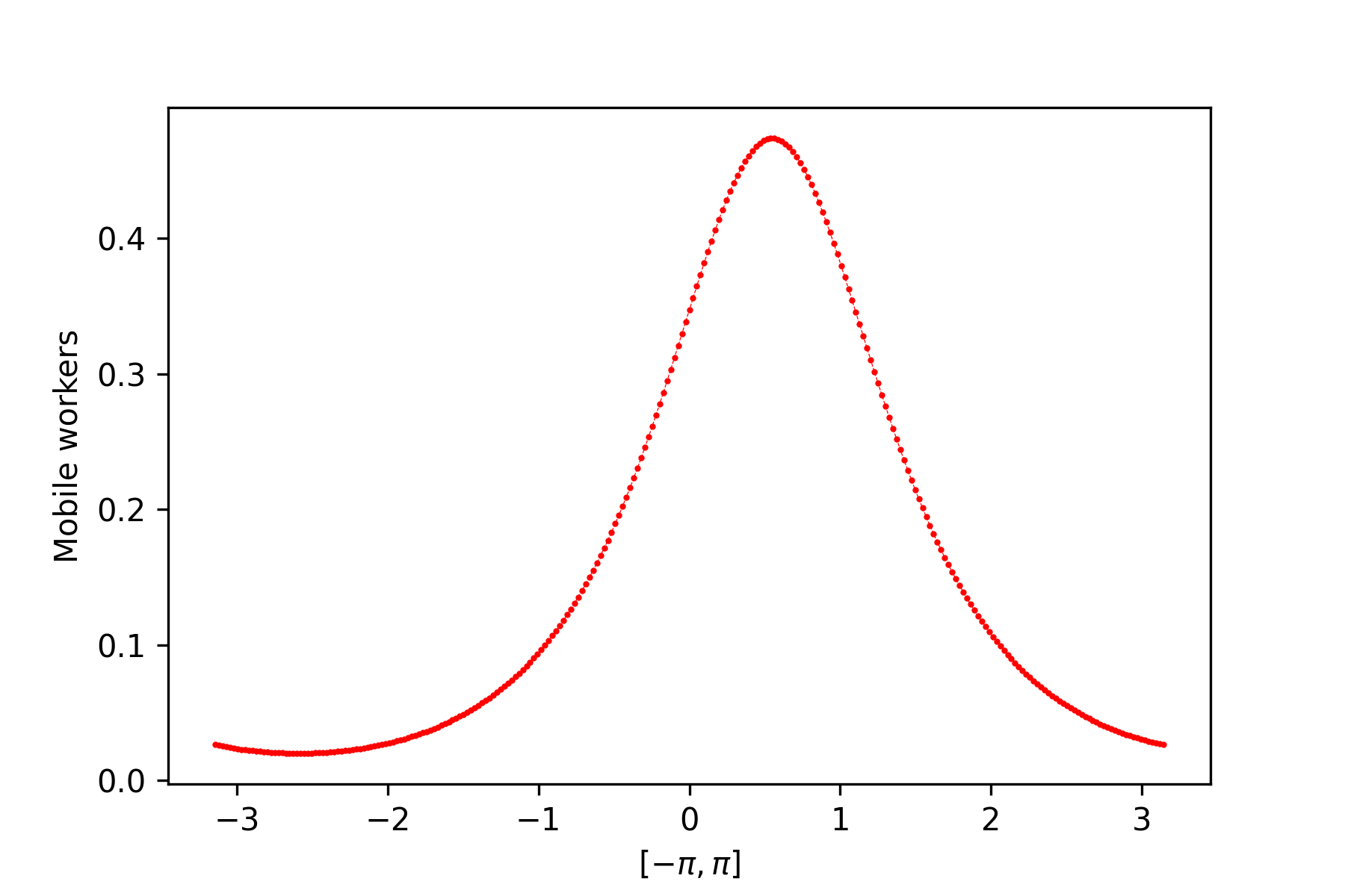
(a) Mobile population density $\lambda^{*}$

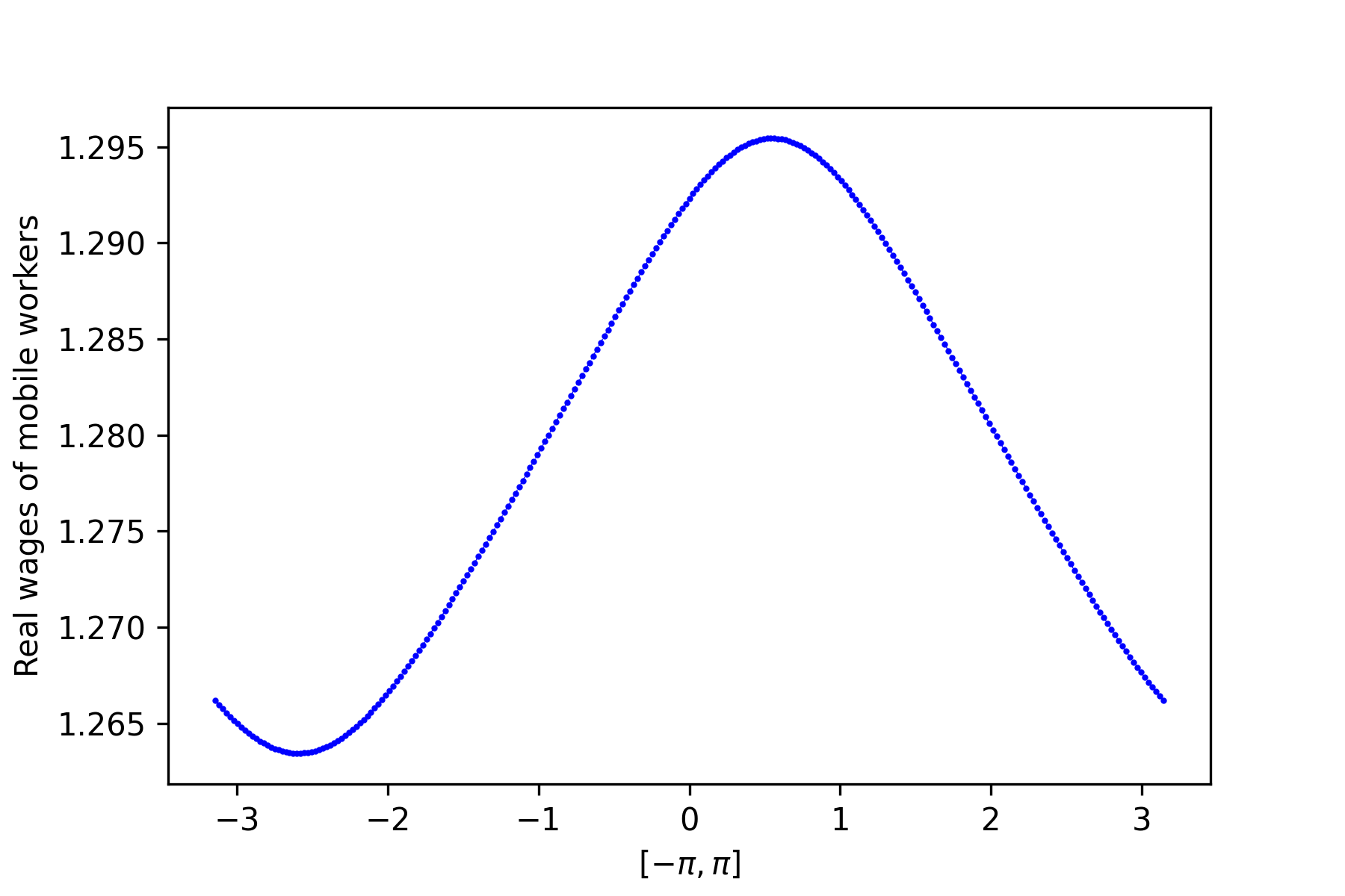
(b) Real wage $\omega^{*}$

Figure 2: Stationary state for $(\sigma,\tau)=(5.0,0.05)$

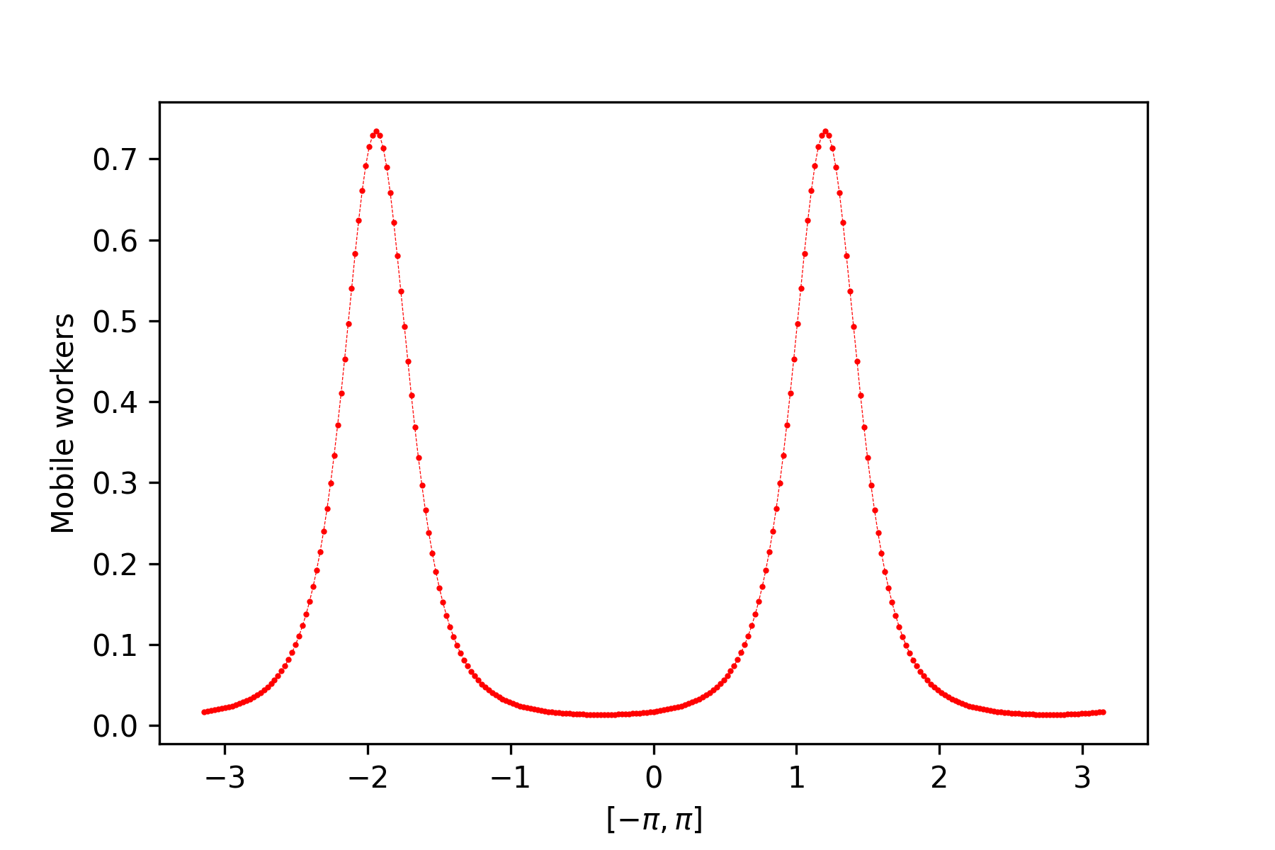
(a) Mobile population density $\lambda^{*}$

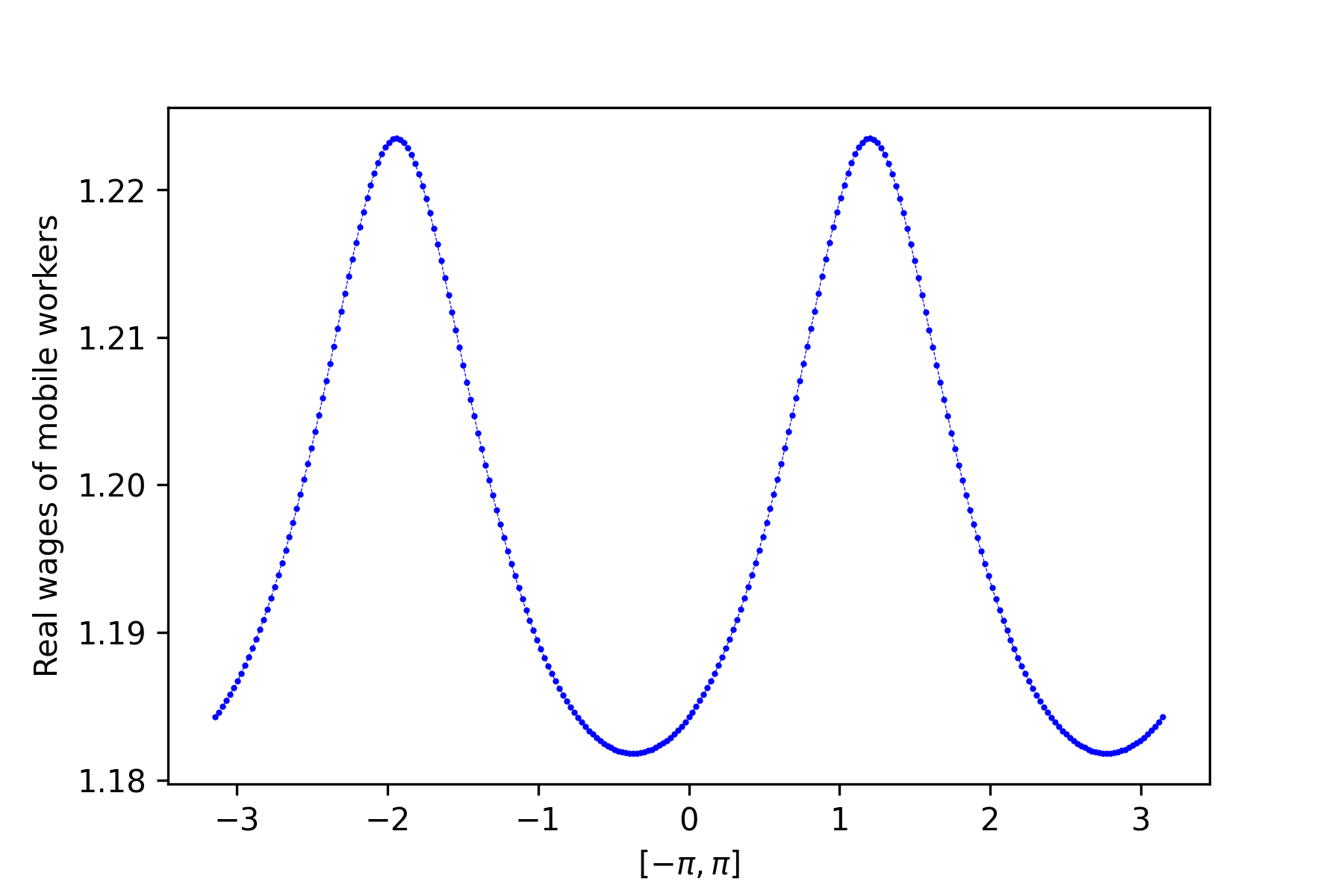
(b) Real wage $\omega^{*}$

Figure 3: Stationary state for $(\sigma,\tau)=(5.0,0.15)$

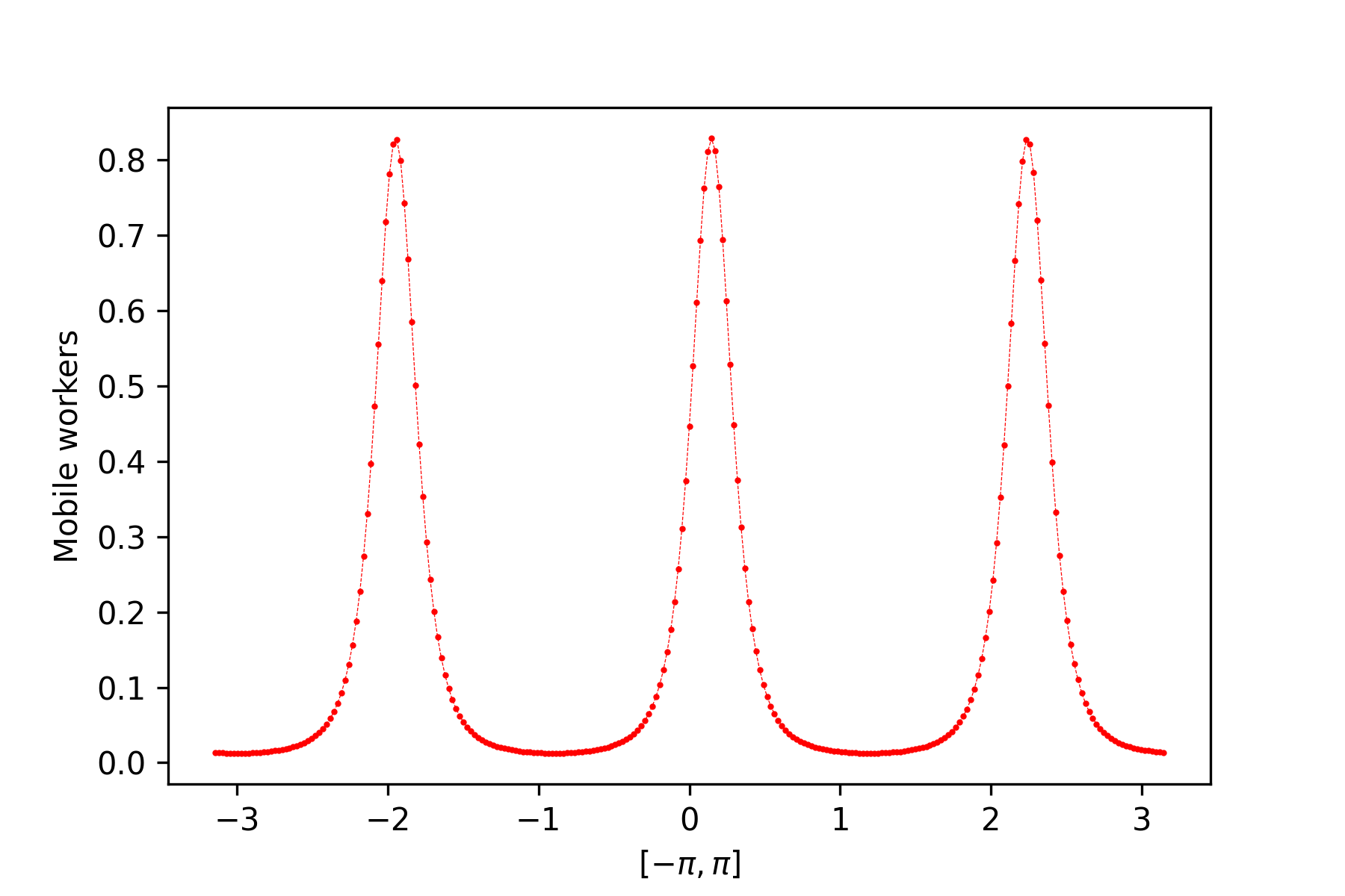
(a) Mobile population density $\lambda^{*}$

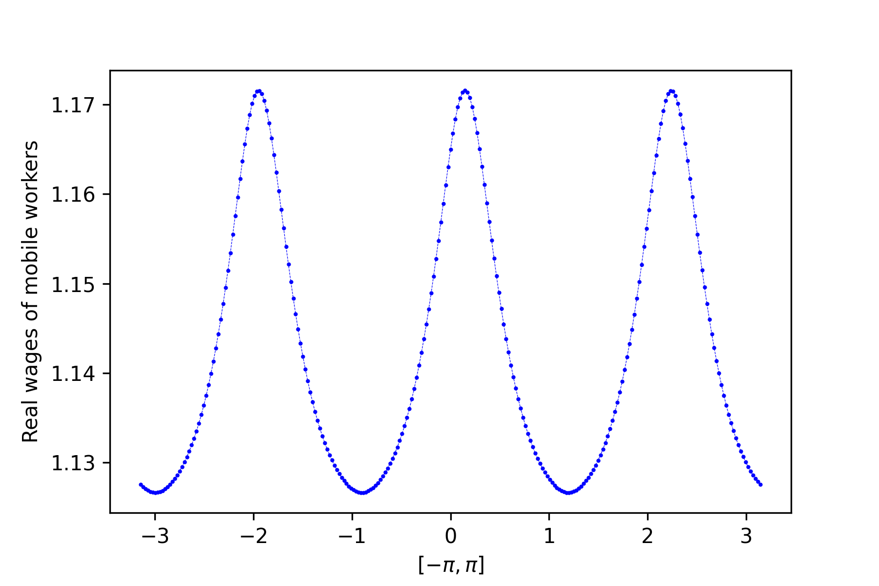
(b) Real wage $\omega^{*}$

Figure 4: Stationary state for $(\sigma,\tau)=(5.0,0.25)$

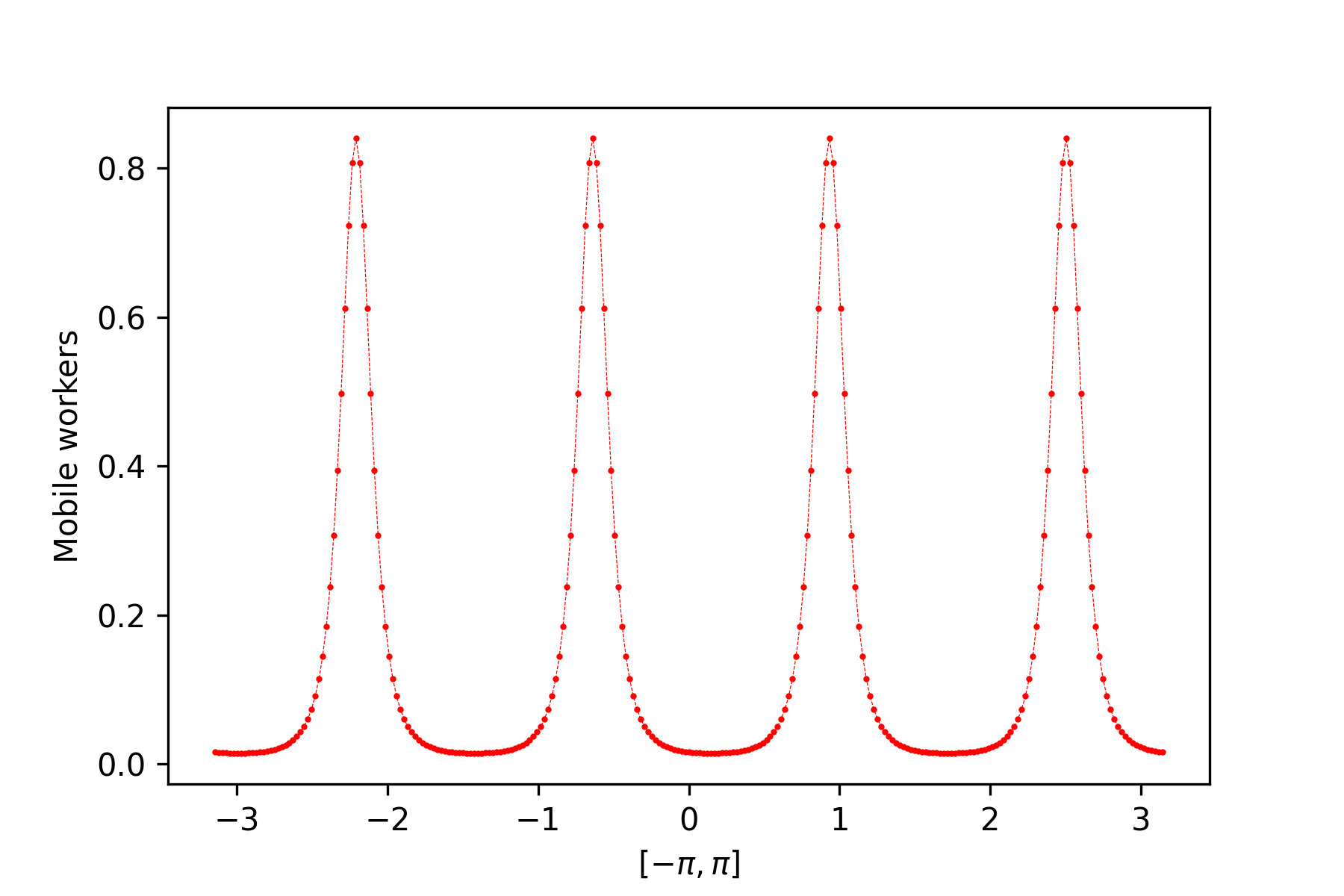
(a) Mobile population density $\lambda^{*}$

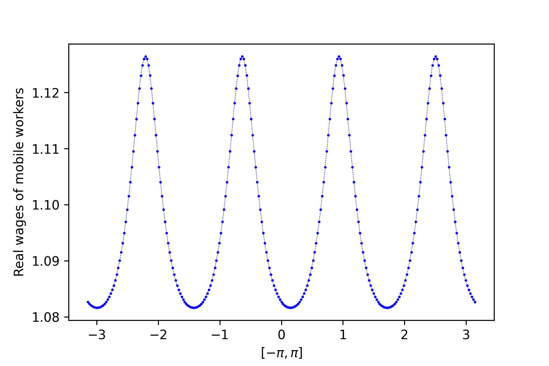
(b) Real wage $\omega^{*}$

Figure 5: Stationary state for $(\sigma,\tau)=(5.0,0.35)$

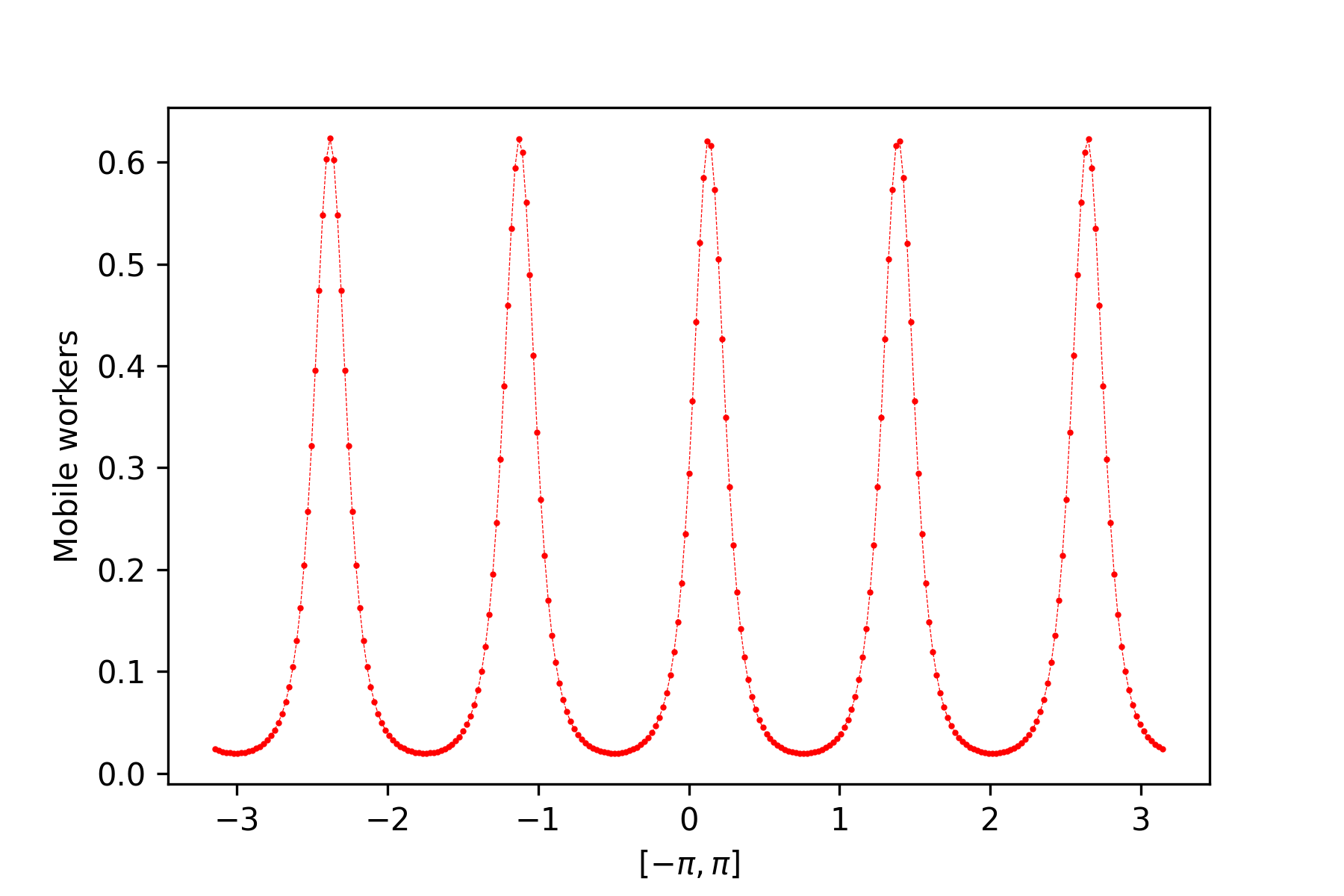
(a) Mobile population density $\lambda^{*}$

(b) Real wage $\omega^{*}$

Figure 6: Stationary state for $(\sigma,\tau)=(5.0,0.37)$

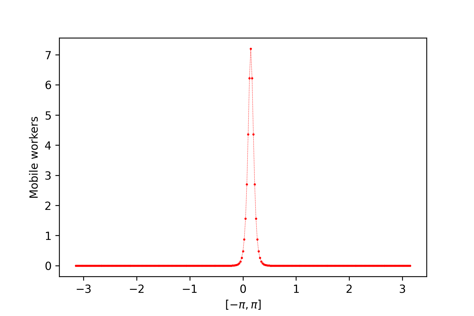
(a) Mobile population density $\lambda^{*}$

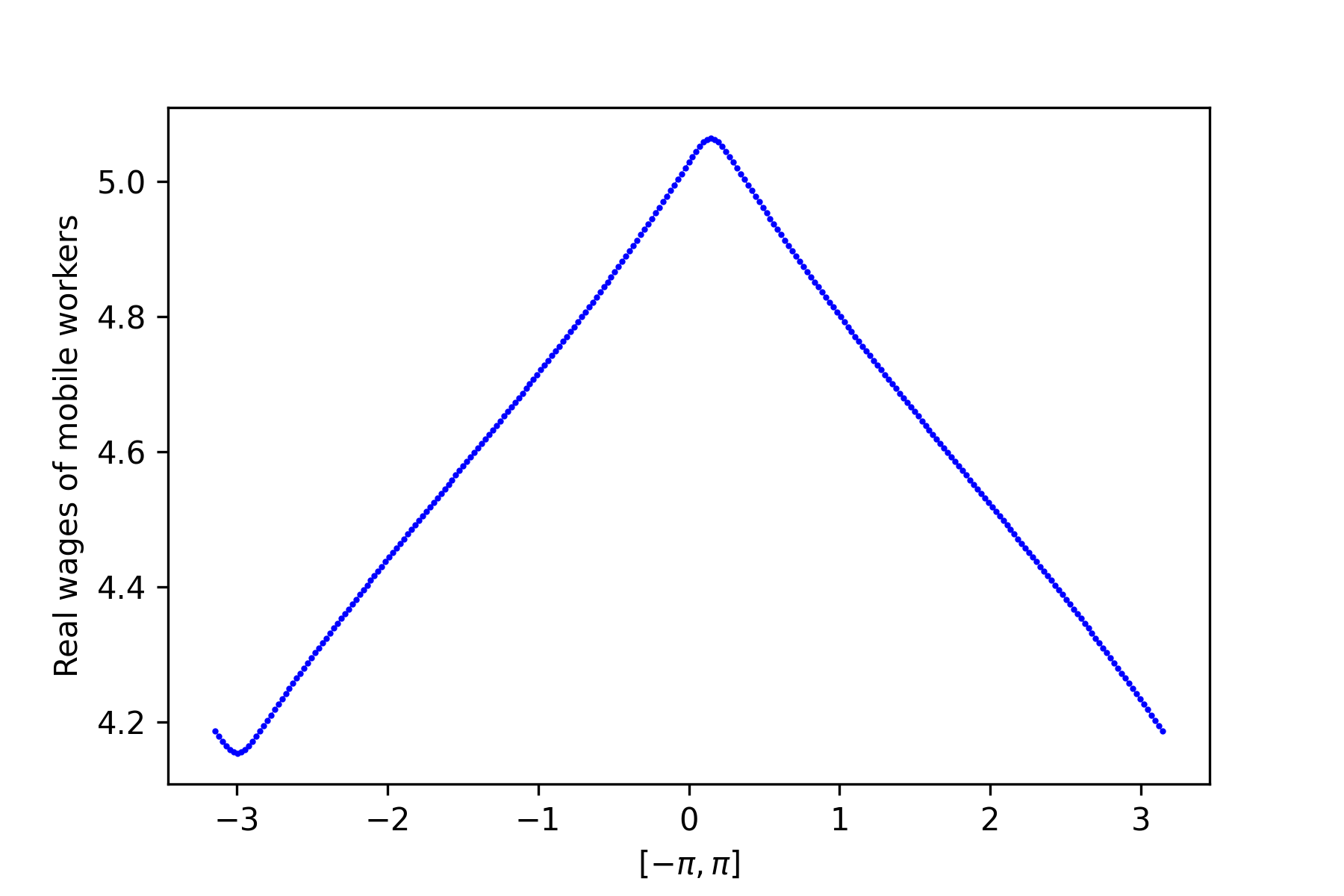
(b) Real wage $\omega^{*}$

Figure 7: Stationary state for $(\sigma,\tau)=(1.3,0.5)$

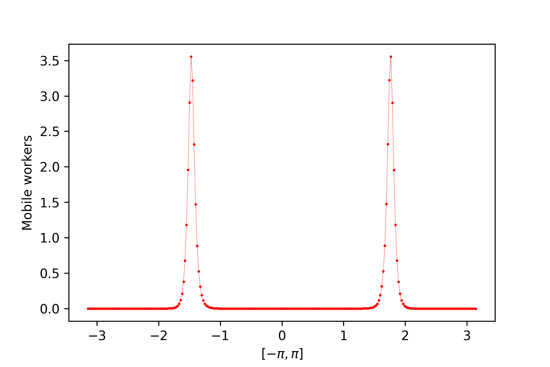
(a) Mobile population density $\lambda^{*}$

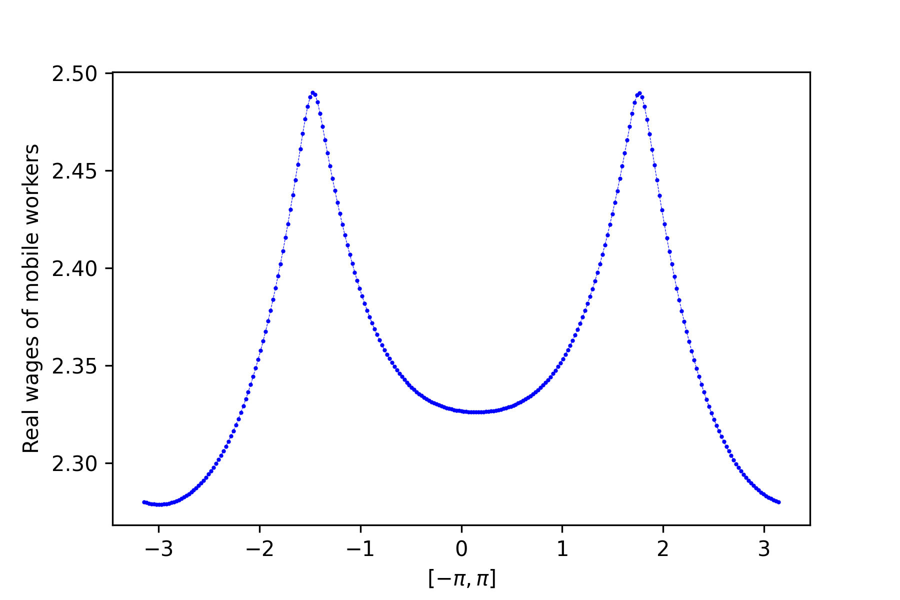
(b) Real wage $\omega^{*}$

Figure 8: Stationary state for $(\sigma,\tau)=(2.4,0.5)$

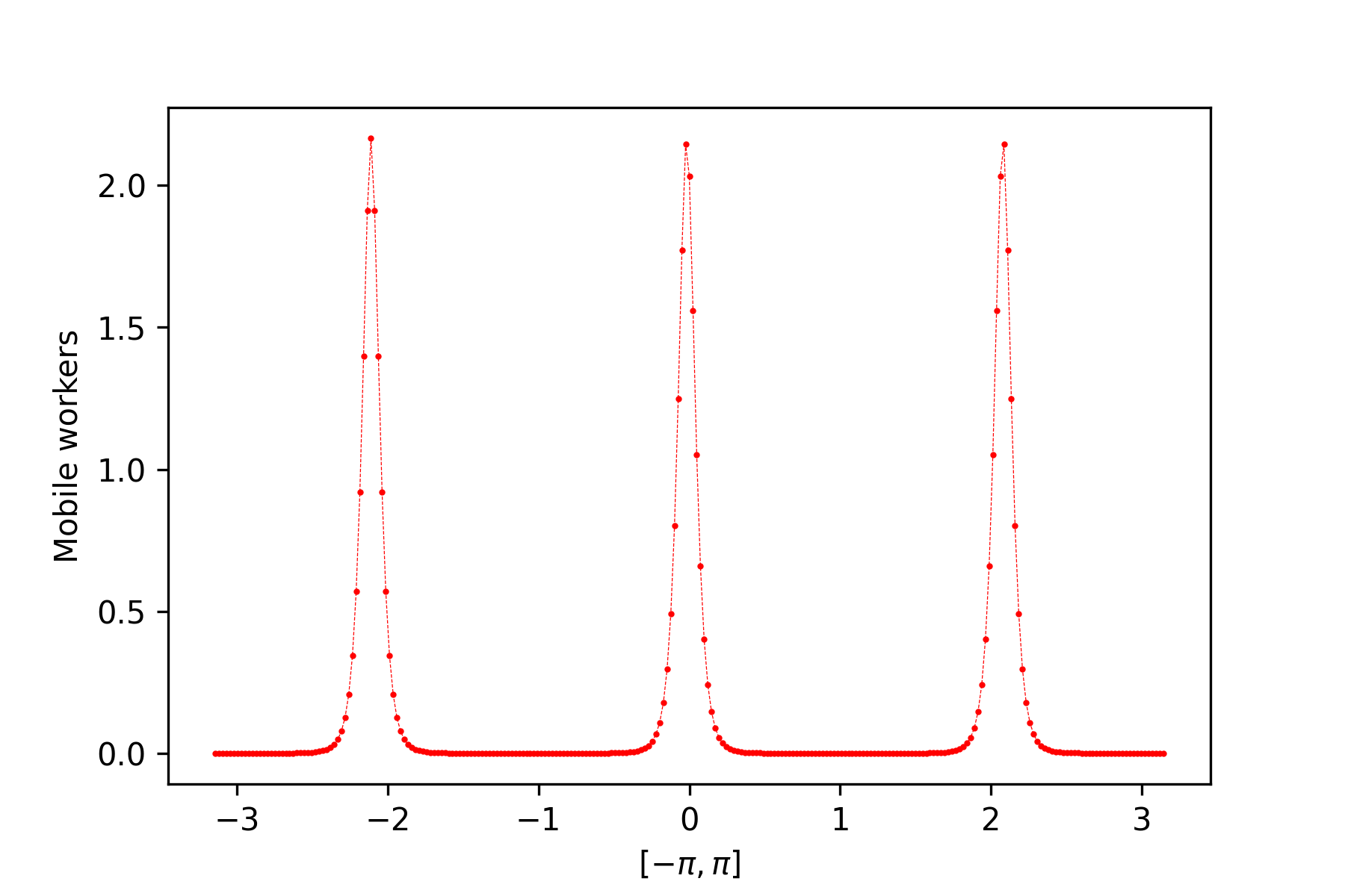
(a) Mobile population density $\lambda^{*}$

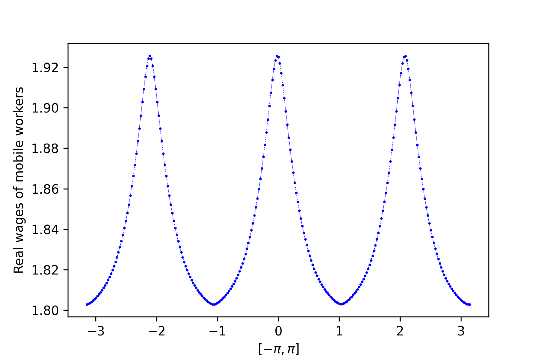
(b) Real wage $\omega^{*}$

Figure 9: Stationary state for $(\sigma,\tau)=(3.0,0.5)$

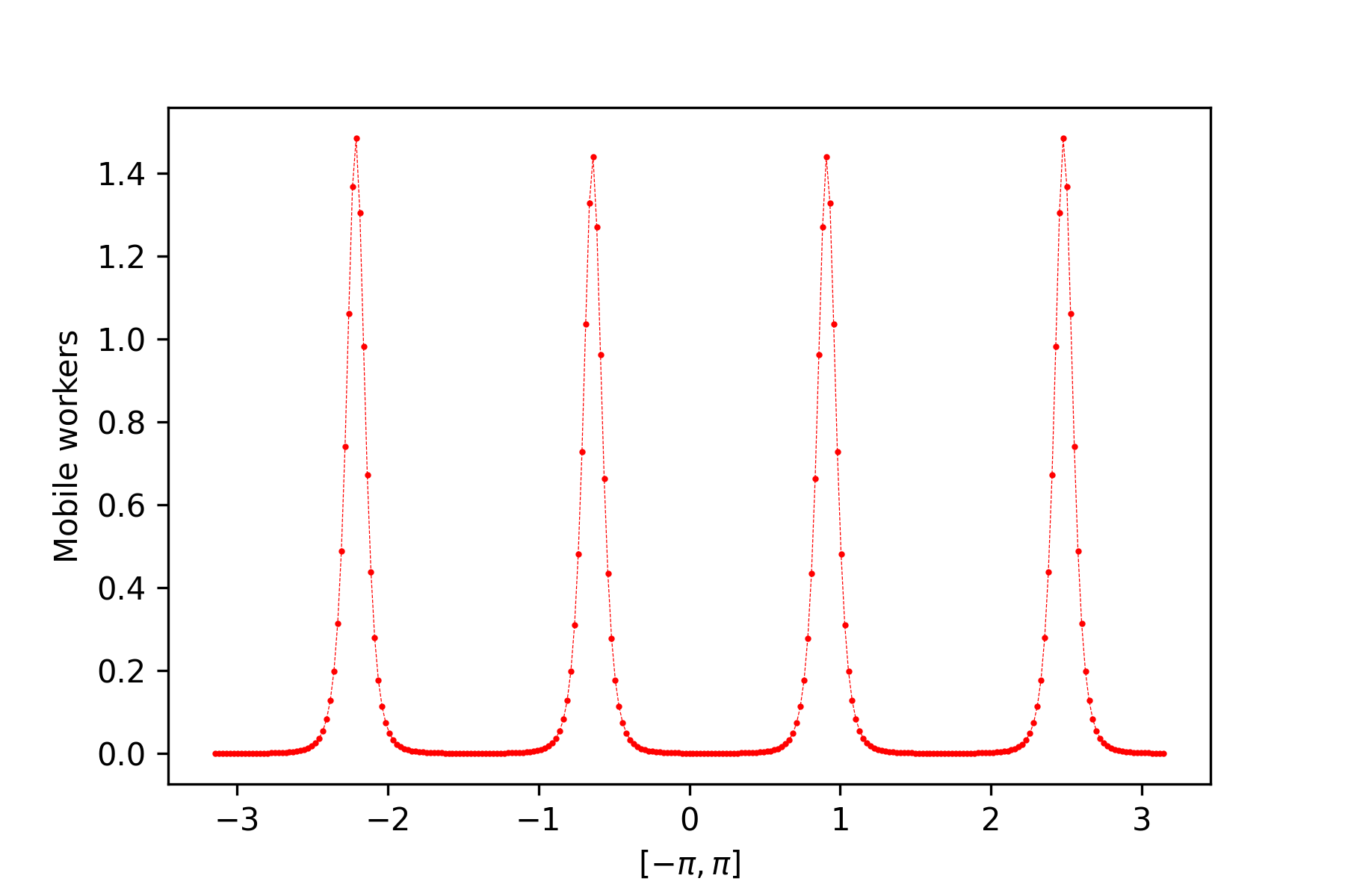
(a) Mobile population density $\lambda^{*}$

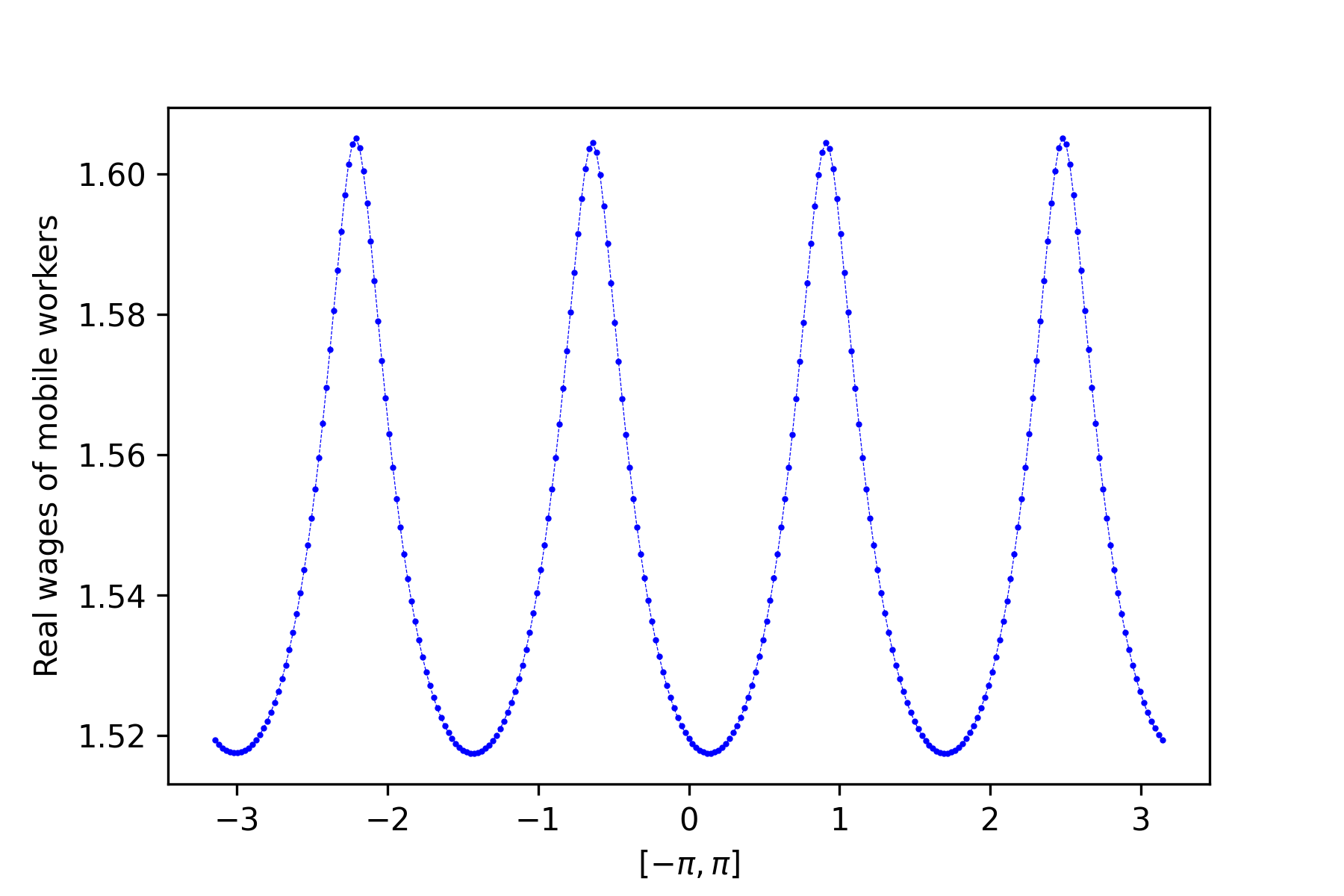
(b) Real wage $\omega^{*}$

Figure 10: Stationary state for $(\sigma,\tau)=(3.5,0.5)$

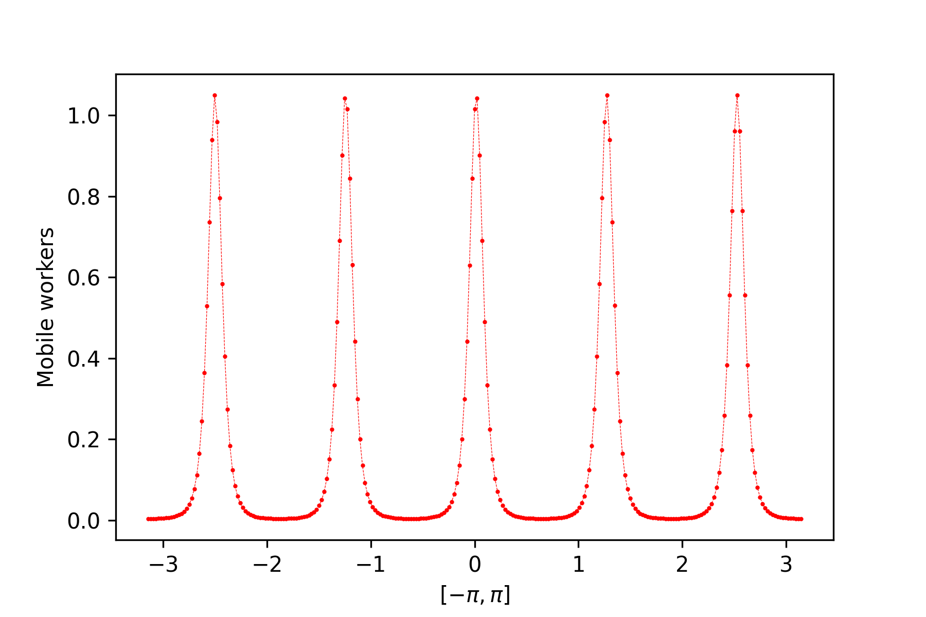
(a) Mobile population density $\lambda^{*}$

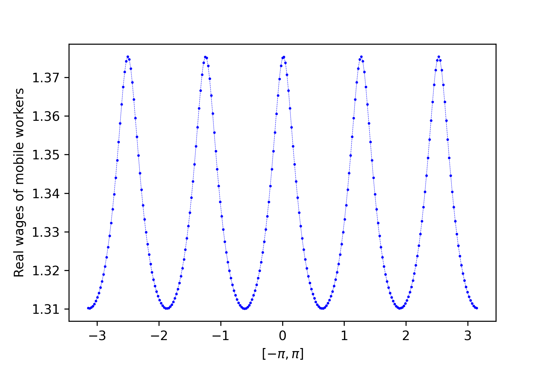
(b) Real wage $\omega^{*}$

Figure 11: Stationary state for $(\sigma,\tau)=(4.0,0.5)$

5 Concluding remarks

In this paper, we propose a NEG model in which population migration is given by a partial differential equation, consider it on a one-dimensional periodic space, analyze the stability of its homogeneous stationary solution, and numerically simulate its asymptotic behavior.

The stability of the homogeneous stationary solution is investigated by adding small perturbations and decomposing them into Fourier series. As the transport costs become lower or the preference for variety becomes stronger, a mode with a higher frequency is found to get destabilized first. In other words, modes with lower frequencies do not get destabilized until the transport costs are sufficiently lowered or the preference for variety becomes sufficiently strong.

From the numerical simulation, it is observed that such destabilized solutions eventually converge to distributions having several urban areas. The number of the urban areas thus formed decreases with the decreasing transport costs or with the strengthening preference for variety.

Modeling population migration in terms of advection, which means that population can only migrate within a small neighborhood, and diffusion, which means that population migrate for non-economic motives as well, is useful when considering real world economy. The model and the method of computing its solution proposed in this paper would provide a theoretical tool for studying regional economic phenomena involving advection and diffusion.

6 Appendix

6.1 Derivation of the advection-diffusion model

Let $\mathbb{J}:(t,x)\in[0,\infty)\times\Omega\to\mathbb{J}(t,x)\in\mathbb{R}^{n}$ be an $n$-dimensional vector field, where $n\in\mathbb{N}$, representing the velocity of the migration of mobile workers. By using the well-known method relying on the divergence theorem, we obtain the following conservation equation

$$\frac{\partial\lambda}{\partial t}(t,x)+\nabla\cdot\mathbb{J}(t,x)=0,$$ (28)

where $\nabla\cdot\mathbb{J}(t,x)$ denotes the divergence of the vector $\mathbb{J}(t,x)$ with respect to the space variable $x$.

Various models can be derived by linking this vector field $\mathbb{J}$ to the migration behavior of mobile workers. The following procedure is similar to that used in Murray (2002, Section 11.4) to derive a reaction-diffusion-chemotaxis equation. Let mobile workers migrate in the direction of increasing real wages in space. Additionally, the size of migrating population is assumed to be proportional to the size of the mobile population at the departure region. As a result, we have a vector field $\mathbb{J}_{\text{adv}}$ such that

$$\mathbb{J}_{\text{adv}}(t,x)=a\lambda(t,x)\nabla\omega(t,x),~{}a>0,$$

where $\nabla\omega(t,x)$ is the gradient of $\omega(t,x)\in\mathbb{R}^{n}$ with respect to $x$. Meanwhile, mobile workers escape from a more populated region to a less populated area. This can be expressed as a vector field $\mathbb{J}_{\text{diff}}$ such that

$$\mathbb{J}_{\text{diff}}(t,x)=-d\nabla\lambda(t,x),~{}d>0,$$

where $\nabla\lambda(t,x)\in\mathbb{R}^{n}$ is the gradient of $\lambda(t,x)$ with respect to $x$. Putting $\mathbb{J}$ in (28) as $\mathbb{J}=\mathbb{J}_{\text{adv}}+\mathbb{J}_{\text{diff}}$, we have

$$\frac{\partial\lambda}{\partial t}(t,x)+a\nabla\cdot\left(\lambda(t,x)\nabla\omega(t,x)\right)=d\Delta\lambda(t,x),$$

where $\Delta$ stands for the Laplace operator with respect to $x$.

6.2 The variable $Z_{k}$

A careful calculation shows that

$$\int_{-\pi}^{\pi}e^{iks}e^{-\alpha D(\rho r,\rho s)}\rho ds=\frac{2\alpha\rho^{2}\left(1-(-1)^{k}e^{-\alpha\rho\pi}\right)}{k^{2}+\alpha^{2}\rho^{2}}e^{ikr}.$$ (29)

It is easy from (14) and (29) to see that

$$\overline{G}^{\sigma-1}\int_{-\pi}^{\pi}e^{iks}e^{-\alpha D(\rho r,\rho s)}\rho ds=\frac{F}{\overline{\lambda}}Z_{k}e^{ikr}.$$

References

- (1)
- Bezanson et al. (2017) Bezanson, Jeff, Alan Edelman, Stefan Karpinski, and Viral B Shah, “Julia: A fresh approach to numerical computing,” SIAM review, 2017, 59 (1), 65–98.
- Fujita et al. (1999) Fujita, M., P. Krugman, and A. Venables, The Spatial Economy: Cities, Regions, and International Trade, MIT Press, 1999.
- Krugman (1991) Krugman, P., “Increasing returns and economic geography,” J. Polit. Econ., 1991, 99 (3), 483–499.
- Mossay (2003) Mossay, P., “Increasing returns and heterogeneity in a spatial economy,” Reg. Sci. Urban Econ., 2003, 33 (4), 419–444.
- Murray (2002) Murray, J. D., Mathematical Biology I: An Introduction, Springer, 2002.
- Ohtake (2023a) Ohtake, K., “A continuous space model of new economic geography with a quasi-linear log utility function,” Netw. Spat. Econ., 2023, 23 (4), 905–930.
- Ohtake (2023b) , “City formation by dual migration of firms and workers,” arXiv preprint arXiv:2311.05292, 2023.
- Ohtake (2024) , “Continuous space core-periphery model with transport costs in differentiated agriculture,” arXiv preprint arXiv:2206.01040, 2024.
- Ohtake and Yagi (2018) and A. Yagi, “Asymptotic behavior of solutions to racetrack model in spatial economy,” Sci. Math. Jpn., 2018, 81 (1), 65–95.
- Pflüger (2004) Pflüger, M., “A simple, analytically solvable, Chamberlinian agglomeration model,” Reg. Sci. Uuban econ., 2004, 34 (5), 565–573.
- Samuelson (1952) Samuelson, P. A., “The transfer problem and transport costs: the terms of trade when impediments are absent,” Econ. J., 1952, 62 (246), 278–304.
- Strang (2007) Strang, G., Computational Science and Engineering, Wellesley-Cambridge Press, 2007.
- Tabata et al. (2013) Tabata, M., N. Eshima, Y. Sakai, and I. Takagi, “An extension of Krugman’s coreâperiphery model to the case of a continuous domain: existence and uniqueness of solutions of a system of nonlinear integral equations in spatial economics,” Nonlinear Anal. Real World Appl., 2013, 14 (6), 2116–2132.