Particle and wave dynamics of nonlocal solitons in external potentials

Abstract

We study nonlocal bright solitons subject to external spatially nonuniform potentials. If the potential is slowly varying on the soliton scale, we derive analytical soliton solutions behaving like Newtonian particles. If the potential has the form of an attractive delta-like point defect, we identify different dynamical regimes, defined by the relative strength of the nonlocality and the point defect. In these regimes, the soliton can be trapped at the defect’s location, via a nonlinear resonance with a defect mode – which is found analytically– reflected by or transmitted through the defect, featuring a wave behavior. Our analytical predictions are corroborated by results of direct numerical simulations.

This work explores the dynamics of nonlocal bright solitons in slowly varying and point defect external potentials. Analytical and numerical methods confirm soliton behavior similar to Newtonian motion, including parabolic trajectories and harmonic oscillations in linear and parabolic potentials, respectively.

The asymptotic regimes based on defect strength relative to nonlocal nonlinearity are identified. Solitons exhibit wave dynamics (reflection/transmission) when defects dominate, form defect modes when defect and nonlinearity are balanced, and exhibit behavior similar to the local NLS equation when nonlinearity dominates.

Our methodology offers a rather universal perspective on the particle-wave duality of nonlocal solitons and is able to capture the analytical soliton solutions of the relative problem.

1 Introduction

We consider the following one-dimensional (1D) normalized nonlocal nonlinear Schrödinger equation for the complex field $u(x,t)$:

$$iu_{t}+\frac{1}{2}u_{xx}+nu=V(x)u,$$ (1)

where subscripts denote partial derivatives, $V(x)$ is a real external potential, and the function $n(x,t)$ is given by:

$$n(x,t)=\int_{-\infty}^{+\infty}R(x-x^{\prime})|u(x^{\prime},t)|^{2}dx^{\prime}.$$ (2)

Here, the kernel $R(x)$ is a real function, which describes the nonlocal response of the medium; notice that if the response function is singular, i.e., $R(x)=\delta(x)$ (with $\delta(x)$ being the Dirac $\delta$ function) then Eq. (1)reduces to the local nonlinear Schrödinger (NLS) equations, or Gross-Pitaevskii (in the context of Bose-Einstein condensates (BECs) [1]) equation. We assume that Eqs. (1)-(2) are supplemented with homogeneous boundary conditions at infinity, and consider localized in space solutions, i.e., solitons.

The above model may find applications in the dynamics of optical beams in nonlocal nonlinear media. In such a case, $u(x,t)$ represents the complex electric field envelope, $t$ denotes the propagation distance, while the function $n(x,t)$ may play the role of: (a) the nonlinear change of the refractive index (that depends on the light intensity $I=|u|^{2}$) in thermal media [2, 3], (b) the relative electron temperature perturbation in plasmas [4, 5], and (c) the perturbation of the optical director angle from its static value, due to the presence of the light field, in nematic liquid crystals [6, 7]. The considered nonlocal NLS model is also relevant to the physics of quasi-1D dipolar BECs [8], with $u(x,t)$ representing the macroscopic wavefunction, and $V(x)$ being the external trapping potential. The latter, may also be relevant to optics, with $V(x)$ typically accounting for the spatial modulation of the linear part of the refractive index [9].

There exist various studies on the dynamics of solitons in external potentials. A central result in this context is that, for potentials slowly-varying on the soliton scale, the soliton center $x_{0}$ features a particle-like nature, obeying the following Newtonian equation of motion:

$$\frac{d^{2}x_{0}}{dt^{2}}=-\frac{dV(x_{0})}{dx_{0}},$$ (3)

which is consistent with the Ehrenfest theorem of quantum mechanics [10]. In the case of a parabolic potential, $V(x)=(1/2)\Omega^{2}x^{2}$, Eq. (3) implies that the soliton performs a harmonic oscillation of frequency $\Omega$. This result was first found for solitons of the local NLS [11, 12] (see also Refs. [13, 14] and the review [15] for BECs), and later was also shown in the case of nonlocal solitons for the case of thermal media [16], for liquid crystals [6, 7], and generalized to the case of topological defects [17]. Notice that one of the first explored type of spatial solitons in liquid crystals was actually propagating in an external potential written by the applied voltage [18]. Newtonian equations of motion, similar to (3), were also derived for solitons in trapped dipolar BECs by means of a variational approximation [19]. Furthermore, more recently, the use of external potentials in nonlocal NLS systems have been proposed as a means to control and manipulate nonlinear waves [20, 21, 22].

On the other hand, soliton dynamics have also been studied in the case where the soliton’s spatial width is much smaller than the characteristic spatial scale of the external potential [23]. The most prominent and relevant example in such settings corresponds to the case where the potential takes the form of a point impurity (or defect) of strength $\epsilon$, namely $V(x)=-\epsilon\delta(x)$. Pertinent soliton-impurity collisions where first studied in the context of the local NLS equation in various works —see, e.g., Refs. [11, 24, 25, 26]— and later for the nonlocal setting of dipolar BECs [19]. It was shown that, if the point impurity is attractive ($\epsilon>0$), and if the soliton velocity is small while $\epsilon$ is sufficiently large, then solitons can be trapped at the impurity location; i.e., a nonlinear resonance of the soliton with a defect mode (the nonlinear analogue of the bound state occurring in the linear Schrödinger equation [10]) takes place. This trapping, can also be accompanied by the splitting of the incoming soliton into a reflected and a transmitted part. Hence, in this case, where the potential has the form of a point impurity, the soliton follows a wave behavior upon its interaction with the impurity. Generally, the soliton may behave either as particles or as waves in external potentials, thus featuring a particle-wave duality (see discussion in Refs. [11, 27]), depending on the relative widths of the soliton and the external potential. This behavior was observed also experimentally in nonlocal media, namely in lead glasses featuring a thermal nonlinearity [16] and in nematic liquid crystals across boundaries [28].

Here, in the framework of Eq. (1), we consider bright sech²-shaped nonlocal solitons (see Ref. [29] for this type of solitons), and study their particle and wave dynamics. We introduce an analytical approach, combined with asymptotic and numerical techniques, which complements previous work in the contexts of both local and nonlocal NLS models; for the latter, different settings and methods have been considered [6, 7, 16, 17, 19, 28]. Exploiting the existence of exact analytical soliton solutions of the nonlocal NLS (1) for a specific form of $R(x)$, we present results which, although qualitatively similar to existing ones, refer to a wide class of nonlocal systems, including thermal media, plasmas and nematic liquid crystals, as mentioned above. Thus, our work offers a novel, quite general methodology and provides a rather universal picture for the nonlocal solitons’ particle-wave duality. A brief description of our findings and the organization of our presentation is as follows.

First, in Sec. II we revisit the derivation of the nonlocal soliton solutions of Eq. (1) for $V(x)=0$. Then, we study soliton dynamics in the presence of the potential $V(x)$ and investigate, in particular, the following cases:

• $V(x)$ is varying slowly on the soliton scale (Sec. III),

• the spatial scale of $V(x)$ is much smaller than that of the soliton; for the latter case, we specifically assume that $V(x)=-\epsilon\delta(x)$ (Sec. IV).

To study case (i), we devise an analytical methodology, relying on the use of the hydrodynamic form of the model and an approach resembling the adiabatic perturbation theory for solitons [30, 31], to derive approximate soliton solutions in the presence of $V(x)$. We show that these solitons behave as particles, following Newtonian dynamics, with the evolution of their center obeying Eq. (3). For case (ii), we identify three different asymptotic regimes, pertinent to the nonlocality and the external potential scale competition: in particular, these regimes are defined by the relative strength of the defect and the nonlocality parameter $d$. Then, for each of them, we investigate soliton-defect interactions, and find the following:

• If the defect dominates nonlinearity, the soliton features wave dynamics, being reflected by or transmitted through the defect, closely following dynamics governed by the linear Schrödinger equation (see Refs. [24, 19] for the local and nonlocal NLS setting, respectively).

• If the roles of the defect and the nonlinearity are of equal importance, we analytically determine a defect mode solution, and using numerical simulations, we find that the soliton-defect collision may lead to either complete trapping of the soliton by the defect or partial reflection and transmission, accompanied by partial trapping of the soliton.

• If the nonlinearity dominates the effect of the impurity, we find that, similarly to the case of the local NLS, fast solitons are transmitted through the defect, while slow solitons are captured in the vicinity of the defect, and perform long-lived oscillations.

Finally, in Sec.V we summarize our findings and discuss directions for future work.

2 Nonlocal bright solitons

We now focus on a specific form of the nonlocality, such that the kernel $R(x)$ is a real, positive definite, localized and symmetric function, obeying the normalization condition $\int_{-\infty}^{+\infty}R(x)dx=1$. We consider in particular the following form of the kernel, which is relevant to the evolution of an electromagnetic beam in a nonlocal nonlinear medium [2, 3, 4, 5, 6, 7] (see also [32, 33, 34] and references therein):

$$R(x)=\frac{1}{2d}\exp\left(-\frac{|x|}{d}\right).$$ (4)

Here, $d>0$ is a spatial scale accounting for the degree of nonlocality (for $d\rightarrow 0$ the function $R(x)$ becomes singular, and Eq. (1) reduces to the NLS with a local nonlinearity). In this case, using Fourier transforms, it can be shown (see, e.g., Ref. [35]) that Eq. (1) can be expressed as the following system of partial differential equations (PDEs):

$$iu_{t}+\frac{1}{2}u_{xx}+nu=V(x)u,$$ (5)

$$d^{2}n_{xx}-n+|u|^{2}=0.$$ (6)

We consider at first the case where the potential is absent, i.e., $V(x)=0$, with our aim being in discussing the possible form of solitons solutions that can be supported by Eqs. (5)-(6). Such nonlocal solitons can typically be found in approximate form (see, e.g., Refs. [36, 37]), featuring a shape that depends on the degree of nonlocality, namely ranging from a sech-profile (in the local case, with $d\rightarrow 0$) to a Gaussian profile (in the highly nonlocal case, with $d\rightarrow\infty$). Nevertheless, for a fixed and finite value of the nonlocality parameter $d$ (which, as will be seen, controls the soliton amplitude —and power), exact analytical sech²-shaped soliton solutions of Eqs. (5)-(6) are possible —see Ref. [29] and references therein.

Let us now revisit the derivation of the aforementioned exact soliton solutions which, for simplicity, will first be derived in a stationary form. We introduce the ansatz:

$$u=u_{0}(x)\exp[i\omega_{0}(t+\sigma_{0})],\quad n=n_{0}(x),$$ (7)

where $u_{0}(x)$ is an unknown real function, $\omega_{0}$ is the unknown frequency of the solution, while $\sigma_{0}$ is an arbitrary real parameter representing the initial phase of the soliton. Substituting Eqs. (7) into Eqs. (5)-(6) (for $V(x)=0$), we arrive at the following system of ordinary differential equations (ODEs):

$$u_{0}^{\prime\prime}-2\omega_{0}u_{0}+2u_{0}n_{0}=0,$$ (8)

$$d^{2}n_{0}^{\prime\prime}-n_{0}+u_{0}^{2}=0,$$ (9)

with primes denoting differentiation with respect to $x$. Then, observing that if:

$$n_{0}=\frac{1}{\sqrt{2}d}u_{0},\quad{\rm and}\quad\omega_{0}=\frac{1}{2d^{2}},$$ (10)

then the system (8)-(9) reduces to a single ODE:

$$u_{0}^{\prime\prime}-2\omega_{0}u_{0}+\sqrt{\frac{2}{d}}u_{0}^{2}=0.$$ (11)

Then, the exact solution $u_{0}(x)=\frac{3}{2\sqrt{2}d}{\rm sech}^{2}\left(\frac{x-x_{0}}{2d}\right)$ of the latter (with $x_{0}$ being the initial location, or the center of the pulse), gives rise to the following nonlocal bright soliton solutions of Eqs. (5)-(6):

$$u(x,t) = \frac{3}{2\sqrt{2}d}{\rm sech}^{2}\left[\frac{1}{2d}(x-x_{0})\right]e^{i\omega_{0}(t+\sigma_{0})},$$ (12)

$$n(x,t) = \frac{3}{4d^{2}}{\rm sech}^{2}\left[\frac{1}{2d}(x-x_{0})\right].$$ (13)

Apart from stationary solutions, traveling soliton solutions exist as well, and can be constructed by means of a Galilean boost. Indeed, it is straightforward to see that if $u_{s}(x,t)$, $n_{s}(x,t)$ is a stationary solution of Eqs. (5)-(6) for $V(x)=0$, then a traveling wave solution of these equations is of the form:

$$u(x,t) = u_{s}(x-kt,t)\exp\left[i\left(kx-\frac{1}{2}k^{2}t\right)\right],$$ (14)

$$n(x,t) = n_{s}(x-kt,t),$$ (15)

where $k$ is a free parameter characterizing the velocity, wavenumber and frequency of the traveling solution. Hence, using Eqs. (14)-(15) and Eqs. (12)-(13), we find that the traveling soliton solutions of Eqs. (5)-(6), for $V(x)=0$, are:

$$\!\!\!\!\!\!\!u(x,t) = \frac{3}{2\sqrt{2}d}{\rm sech}^{2}\left[\frac{1}{2d}(x-kt-x_{0})\right]e^{i\phi(x,t))},$$ (16)

$$\!\!\!\!\!\!\!\phi(x,t) = kx-\frac{1}{2}\left(k^{2}-\frac{1}{d^{2}}\right)t+\sigma_{0},$$ (17)

$$\!\!\!\!\!\!\!n(x,t) = \frac{3}{4d^{2}}{\rm sech}^{2}\left[\frac{1}{2d}(x-kt-x_{0})\right].$$ (18)

3 Solitons in slowly-varying potentials

We now consider the full problem where the potential is present, and consider at first the case of slowly-varying potentials. In particular, we will study the case where the soliton width, characterized by the nonlocality parameter $d$ [see Eqs. (16)-(18)] is such that:

$$d\ll W,$$ (19)

where $W$ is the characteristic scale of the inhomogeneity of $V(x)$. We wish to show that, in this case, the problem admits a bright soliton solution, of a form similar to that given in Eqs. (16)-(18), but with the soliton’s center, wavenumber and phase being functions of time; the explicit form of these functions, together with the soliton shape, will be determined below in a self-consistent manner. Notice that our approach is reminiscent to the adiabatic approximation in the perturbation theory for solitons [30, 31], which is commonly used in problems involving perturbed NLS models.

To proceed, we separate the real and imaginary parts in Eq. (5) using the ansatz $u(x,t)=f(x,t)\exp[i\theta(x,t)]$, where $f(x,t)$ and $\theta(x,t)$ are real functions. This way, we obtain from Eqs. (5)-(6) the following system of PDEs:

$$\left(f^{2}\right)_{t}+\left(f^{2}\theta_{x}\right)_{x}=0,$$ (20)

$$f_{xx}-\left[2\theta_{t}+\theta_{x}^{2}+2V(x)\right]f+2nf=0,$$ (21)

$$d^{2}n_{xx}-n+f^{2}=0.$$ (22)

Notice that, in fact, Eqs. (20) and (21) constitute the hydrodynamic form of Eq. (5), with (20) being the continuity equation (conservation of mass) and (21) having the form of an Euler equation (conservation of momentum). Next, to further simplify the above system, we assume that the functions $f$ and $\theta$ are of the form:

$$f=f(\xi),\quad\xi\equiv x-X_{0}(t),\quad\theta=K(t)x-\varphi_{0}(t),$$ (23)

where $X_{0}(t)$ represents the location of the maximum of the function $f$, while $K(t)$ and $\varphi_{0}(t)$ denote, respectively, the wavenumber and time-dependent phase of the solution; all the above are unknown functions, to be determined. Then, substituting Eq. (23) into Eqs. (20)-(22), we find the following. First, Eq. (20) leads to the result:

$$K(t)=\dot{X}_{0},$$ (24)

with overdot denoting differentiation with respect to $t$. Second, Eq. (21) becomes:

$$f_{\xi\xi}-2\Omega_{0}f+2nf=0,$$ (25)

where the function $\Omega_{0}(x,t)$ is given by:

$$\Omega_{0}(x,t)=-\dot{\varphi}_{0}+\ddot{X_{0}}x+\frac{1}{2}\dot{X}_{0}^{2}+V(x).$$ (26)

We now observe that the system of Eqs. (25) and (22) has a form similar to that of Eqs. (8)-(9), but with the important difference that Eq. (25) features the coefficient $\Omega_{0}$ which depends both on space $x$ and time $t$. This fact indicates that, under certain conditions, soliton solutions similar to those given in Eqs. (16)-(18) may also be supported by Eqs. (25) and (22), i.e., even in the presence of the external potential.

To identify such conditions, first we notice that the spatial dependence of this coefficient may be suppressed upon assuming that the potential $V(x)$ varies slowly over the width of the density of the solution. To see this, we Taylor expand the potential around $X_{0}$, namely:

$$V(x)=V(X_{0})+\frac{dV}{dX_{0}}(x-X_{0})+\frac{1}{2}\frac{d^{2}V}{dX_{0}^{2}}(x-X_{0})^{2}+\cdots,$$

where $dV/dX_{0}=dV/dx\big{|}_{x=X_{0}}$ and so on. Then, for a slowly varying potential [see Eq. (19)], we may keep in the Taylor expansion solely the linear terms in $(x-X_{0})$. Substitution of these terms into Eq. (26) leads to the following expression of $\Omega_{0}$:

$$\Omega_{0}(x,t)=-\dot{\varphi}_{0}+\left[\ddot{X_{0}}+\frac{dV}{dX_{0}}\right]x+\left[\frac{1}{2}\dot{X}_{0}^{2}+V(X_{0})\right]-X_{0}\frac{dV}{dX_{0}}.$$ (27)

It is now straightforward to see that as long as $\Omega_{0}$ depends only on time, the soliton center evolves according to the Newtonian equation of motion:

$$\ddot{X_{0}}=-\frac{dV}{dX_{0}},$$ (28)

a result which is identical to the one corresponding to the local NLS [see Eq. (3)]. Thus, in the nonlocal problem under consideration, we again obtain a result consistent with the Ehrenfest theorem. Notice that the quantity in the second square bracket in the right-hand side of Eq. (27) represents the total energy $E_{0}$ of the pertinent dynamical system, namely:

$$E_{0}=\frac{1}{2}\dot{X}_{0}^{2}+V(X_{0})=\frac{1}{2}\dot{X}_{0}^{2}(0)+V(X_{0}(0)),$$ (29)

which remains constant for all $t$, taking a value determined by the initial velocity $\dot{X}_{0}(0)$ and initial location $X_{0}(0)$ of the solution.

According to the above, we arrive at the following expression for $\Omega_{0}=\Omega_{0}(t)$ in Eq. (25):

$$\Omega_{0}=-\dot{\varphi}_{0}+E_{0}-X_{0}\frac{dV}{dX_{0}},$$ (30)

and impose the requirement $\Omega_{0}(t)={\rm const.}$ This is in accordance to the line of the analysis of the previous Section [for Eqs. (8) and (9)], and leads to conditions rendering Eqs. (25) and (22) identical. Obviously, these conditions are similar to the ones in Eq. (10), namely:

$$n=\frac{1}{\sqrt{2}d}f,\quad{\rm and}\quad\Omega_{0}=\frac{1}{2d^{2}},$$ (31)

where the second of the above equations can be used to determine the unknown function $\varphi_{0}(t)$. The latter, is given by:

$$\varphi_{0}(t)=\left(E_{0}-\frac{1}{2d^{2}}\right)t+\int_{0}^{t}X_{0}(s)\frac{dV}{dX_{0}}ds.$$ (32)

To this end, summarizing the above results, we can arrive at the following expressions for the nonlocal bright solitons in external potentials:

$$\!\!\!\!\!\!\!u(x,t) = \frac{3}{2\sqrt{2}d}{\rm sech}^{2}\left[\frac{1}{2d}\left(x-X_{0}(t)\right)\right]e^{i\varphi(x,t))},$$ (33)

$$\!\!\!\!\!\!\!\varphi(x,t) = \dot{X}_{0}(t)x-\varphi_{0}(t),$$ (34)

$$\!\!\!\!\!\!\!n(x,t) = \frac{3}{4d^{2}}{\rm sech}^{2}\left[\frac{1}{2d}\left(x-X_{0}(t)\right)\right],$$ (35)

where the soliton center $X_{0}(t)$ obeys the Newtonian equation of motion (28), and $\varphi_{0}(t)$ is given by Eq. (32).

We proceed by presenting results of direct numerical simulations. In particular, we evolve Eqs. (5)-(6) using Eqs. (33)-(35) for $t=0$ as initial conditions, considering two different types of the external potential: a linear and a parabolic one, and compare the numerical results with our analytical predictions.

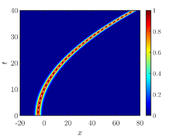
Figure 1: Contour plot showing the evolution of the modulus $|u(x,t)|$ of a nonlocal bright soliton in the presence of the linear (gravitational-type) potential [Eq. (36)]. The dashed line depicts the soliton trajectory [Eq. (37)]. Parameter values are $a=-1$, $b=0$, $X_{0}(0)=-5$, and $d=1$.

We start by noting the following. While the expressions (33)-(35) for the soliton profiles are approximate, and are valid for arbitrary potentials varying slowly over the soliton scale, they become exact in the case of linear (gravitational-type) potentials, of the form:

$$V(x)=ax+b,$$ (36)

where $a,b\in\mathbb{R}$. In this case, a soliton subject to such a potential features an accelerating motion: indeed, the soliton center is given by:

$$X_{0}(t)=-\frac{1}{2}at^{2}+X_{0}(0),$$ (37)

and the evolution of the soliton, as obtained from the numerical integration of Eqs. (5)-(6), is depicted in Fig. 1 for parameter values $a=-1$, $b=0$, $d=1$ and $X_{0}(0)=-5$. In this figure, shown is the contour plot of the soliton modulus, $|u(x,t)|$ in the $xt$-plane, with the dashed line depicting the analytical prediction of Eq. (37). Observe that the soliton follows the analytically predicted dynamics, in excellent agreement with the numerical finding.

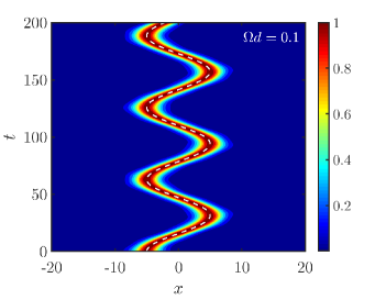
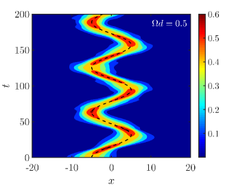
Figure 2: Contour plots showing the evolution of the modulus $|u(x,t)|$ of a nonlocal bright soliton in the presence of the parabolic potential of Eq. (38). The dashed lines depict the soliton trajectory given in Eq. (39). Parameter values are $\Omega=0.1$, $X_{0}(0)=-5$, $\psi_{0}=0$, while $d=1$ or $d=5$ for the left and right panels, respectively.

We now consider the case where the potential has the form of a parabolic trap, with a trap strength $\Omega$, namely:

$$V(x)=\frac{1}{2}\Omega^{2}x^{2}.$$ (38)

In this case, since the characteristic spatial scale of the potential is $W\sim\Omega^{-1}$, the requirement of Eq. (19) is fulfilled for $\Omega d\ll 1$. Hence, as predicted, in this case the solitons perform harmonic oscillations of frequency $\Omega$, with the soliton center being given by:

$$X_{0}(t)=A_{0}\cos(\Omega t+\psi_{0}),$$ (39)

where the amplitude of the oscillation $A_{0}$ and the initial phase $\psi_{0}$ are determined by the initial conditions. This scenario is confirmed by our numerical result shown in the left panel of Fig. 2, where we have used $\Omega=0.1$ and $d=1$ and, hence, $\Omega d=0.1$ (other parameter values are $X_{0}(0)=-5$ and $\psi_{0}=0$). As seen in this figure, not only the trajectory of the soliton center follows the form of Eq. (39) –see dashed line– but also the functional form of the entire soliton structure evolves adiabatically.

On the other hand, if the requirement of Eq. (19) is violated, as, e.g., in the case example with $\Omega=0.1$ and $d=5$ (and thus $\Omega d=0.5$), then our approach ceases to be accurate. In particular, as shown in the right panel of Fig. 2, the soliton is deformed while evolving in the trap: it features a periodic increase (decrease) in its width (amplitude), accompanied by emission of weak radiation, whenever its motion changes direction, and reorganizes its shape in the vicinity of the trap center. Nevertheless, the soliton still performs an oscillatory motion, with the frequency of the oscillation being equal to $\Omega$ (see dashed line in the figure). Notice that other cases with $\Omega d\sim 1$ were studied too (results not shown here); in such cases, a qualitatively similar behavior was found, but with the soliton featuring a stronger deformation, and emitting stronger radiation.

4 Solitons and point defects

In the previous Section, we analyzed the case where the soliton width $d$ is much smaller than the characteristic scale $W$ of the potential [Eq. (19)]. Here, we will consider the case:

$$d\gg W,$$ (40)

with the most prominent example being the scenario of a point-like impurity, or defect, where the external potential has the form of a delta function:

$$V(x)=-\epsilon\delta(x).$$ (41)

Here, $\epsilon>0$ is a free parameter representing the strength of the defect. Notice that the minus sign corresponds to the case of an attractive impurity which, in the context of quantum mechanics, is known to give rise to a bound state [10]. On the other hand, in the nonlinear case, i.e., in the context of the NLS equation, the analogue of this bound state is the so-called “defect mode”. The latter, is a stationary nonlinear state located at the defect, and can be found in an exact analytical form [25].

We identify three different regimes, distinguished by the relative strength of the soliton amplitude —which is determined by the nonlocality parameter, being $\propto 1/d$— and the strength $\epsilon$ of the localized impurity. In particular, we will study the cases corresponding to:

• $\epsilon d\gg 1$ where the effect of impurity dominates nonlinearity (linear Schrödinger regime);

• $\epsilon d\sim 1$ (crossover regime), where the nonlinearity and impurity are of similar strengths;

• $\epsilon d\ll 1$ (nonlinear regime), where the nonlinearity dominates the effect of the impurity.

4.1 Linear Schrödinger regime, $\epsilon d\gg 1$

We start with the regime $\epsilon d\gg 1$, which corresponds to the linear Schrödinger limit: indeed, in this case, the nonlinearity term can be neglected (because $\lim_{d\rightarrow\infty}n(x,t)=0$) and the problem of Eqs. (5)-(6) can be approximated by the linear Schrödinger equation with an attractive delta potential, namely:

$$iu_{t}+\frac{1}{2}u_{xx}=-\epsilon\delta(x)u.$$ (42)

As is well known [10], the above equation features a normalized bound state, of energy $E_{b}=-\epsilon^{2}/2$, which is of the form:

$$u(x,t)=\sqrt{\epsilon}\exp\left({-\epsilon|x|-i\frac{\epsilon^{2}}{2}t}\right),$$ (43)

as well as a continuous spectrum consisting of scattering states, $\propto\exp[{i(kx-\omega t})]$, of wavenumber $k$ and frequency $\omega$. For the scattering states, the reflection and transmission coefficients, $b(k)$ and $a(k)=1+b(k)$ respectively, read (see, e.g., Ref. [24]): $b(k)=-\epsilon/(\epsilon+ik)$, and $a(k)=ik/(\epsilon+ik)$; hence,

$$|b(k)|^{2}=\frac{\epsilon^{2}}{\epsilon^{2}+k^{2}},\quad|a(k)|^{2}=\frac{k^{2}}{\epsilon^{2}+k^{2}},$$ (44)

and it is noted that $|a(k)|^{2}+|b(k)|^{2}=1$.

The above simple analysis suggests the following. Consider a nonlocal soliton, of the form of Eq. (16), initially located sufficiently far from the defect; this soliton, obviously, is an exact solution of the problem. Now assume that this structure moves towards the defect at $x=0$. In the considered regime of $\epsilon d\gg 1$, since we may neglect the nonlinearity, the soliton of Eq. (16) (at $t=0$) can be interpreted by its Fourier transform, meaning that each Fourier component of wavenumber $k$ will independently interact with the defect. In other words, the wavenumber $k$ in Eqs. (44) can be treated as the free parameter of the moving nonlocal soliton and, thus, $|a(k)|^{2}$ and $|b(k)|^{2}$ for the soliton may be approximated by Eq. (44). Furthermore, we may predict that total reflection (transmission) occurs in the limit $\epsilon^{2}\gg k^{2}$ ($\epsilon^{2}\ll k^{2}$). Outcomes involving both reflection and transmission are obviously possible too.

Thus, in this regime, the soliton features a wave behavior (see discussion, e.g., in Refs. [11, 27] for the local and nonlocal NLS respectively), which is highlighted in Fig. 3. In this figure, shown are contour plots of the field $|u(x,t)|$ in the $xt$-plane, as obtained by means of direct simulations; the dashed (white) lines depict the location of the defect. The initial condition in all cases was the soliton of Eq. (16), initially located at $x_{0}=-10$. The strength of the defect and the nonlocality parameter were fixed to the values are $\epsilon=5$ and $d=1$, while the soliton wavenumber (initial momentum) assumed the values $k=0.3$ (left panel), $k=3$ (middle panel) and $k=60$ (right panel). As predicted in our analysis above, the first (third) case corresponds to total reflection (transmission), while the second one leads to both reflection and transmission. Observe that, in this latter case, only a small part of the soliton is captured by the defect, while large parts are reflected and transmitted, with the relevant amounts being predicted fairly well by Eqs. (44); notice that a similar behavior was also found in Ref. [24], but for the local NLS model.

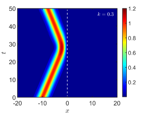
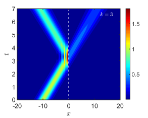
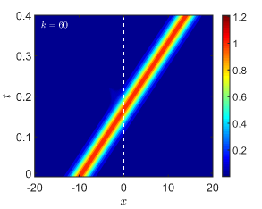
Figure 3: Contour plots showing the evolution of the modulus $|u(x,t)|$ of a nonlocal bright soliton, initially placed at $x_{0}=-10$, for $k=0.3$ (left panel), $k=3$ (middle panel) and $k=60$ (right panel); other parameter values are $\epsilon=5$ and $d=1$, corresponding to the linear Schrödinger regime, $\epsilon d\gg 1$. Dashed (white) line depicts the location of the point defect. From top to bottom, observed are the scenarios of total reflection, partial reflection and partial transmission, and total transmission, as predicted in Eq. (44).

4.2 Crossover regime, $\epsilon d\sim 1$

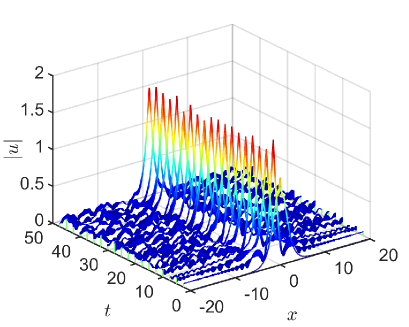
Figure 4: A 3D plot showing the evolution of the modulus $|u(x,t)|$ of a stationary soliton, given by Eq. (12) with $d=1$, when initialized at the location of a point defect of amplitude $\epsilon=0.5$. Observe that the initial soliton emits radiation and eventually reorganizes itself into a defect mode.

Next, we consider the crossover regime, with $\epsilon d\sim 1$, where the effects of the nonlinearity and the impurity play equally important roles in the dynamics. In this case, we may employ our analytical approach of the previous Section to determine, at first, the defect mode for the nonlocal problem under consideration. Our starting point is the system of Eqs. (20)-(22). As we are seeking for a stationary nonlinear state located at $x=0$, we assume that

$$(f^{2})_{t}=0,\quad\theta_{x}=0,\quad\theta_{t}=\omega_{0}=\frac{1}{2d^{2}},$$

as suggested by the exact analytical form of the stationary nonlocal soliton [Eqs. (12)-(13)]. Then, the continuity equation (20) is automatically satisfied, while Eq. (21) takes the form:

$$f_{xx}-2\omega_{0}f+2nf=2\epsilon\delta(x)f.$$ (45)

Requiring continuity of the functions $f$ and $n$ at $x=0$, i.e., $f(0^{-})=f(0^{+})$ and $n(0^{-})=n(0^{+})$, we integrate the above equation from $x=0^{-}$ to $x=0^{+}$, and obtain the jump condition for the first spatial derivative of $f$, namely: $\partial_{x}f(0^{+})-\partial_{x}f(0^{-})=2\epsilon f(0).$ Then, integrating Eqs. (45) and (22) for $x<0$ and $x>0$, we arrive at the following solution, satisfying the above mentioned boundary conditions:

$$f(x)=\frac{3}{2\sqrt{2}d}{\rm sech}^{2}\left[\frac{1}{2d}\left(|x|-\chi_{0}\right)\right],\quad n(x)=\frac{1}{\sqrt{2}d}f(x),$$

where $\chi_{0}=2d{\rm tanh^{-1}}(\epsilon d)$, with $0<\epsilon d<1$. To this end, the defect mode of the nonlocal problem —which is the nonlinear analogue of the bound state of Eq. (43) occurring in the linear Schrödinger limit— is given by:

$$\!\!\!\!\!\!\!\!\!u(x,t) = \frac{3}{2\sqrt{2}d}{\rm sech}^{2}\left[\frac{1}{2d}\left(|x|-\chi_{0}\right)\right]\exp\left(i\frac{1}{2d^{2}}t\right),$$ (46)

$$\!\!\!\!\!\!\!\!\!n(x,t) = \frac{4}{3d^{2}}{\rm sech}^{2}\left[\frac{1}{2d}\left(|x|-\chi_{0}\right)\right].$$ (47)

A simple way to observe the defect mode in the numerical simulations, is to initialize the stationary soliton (12) at $x=0$, i.e., at the location of the point defect. Indeed, in Fig. 4, we observe that as the initial soliton evolves, it emits radiation and is eventually reorganized into the defect mode, which is characterized by a cusp occurring at $x=0$. Here, we have used the parameter values $\epsilon=0.5$ and $d=1$.

In the same regime, it is also interesting to investigate numerically the scattering of a moving soliton from the defect. In particular, first we will consider a case where the moving soliton features a momentum (and energy) less than that of the trapping strength, i.e., with $k<\epsilon$. In the left panel of Fig. 5, shown is the outcome of such a soliton-defect interaction, for $k=0.02$ and $\epsilon=0.5$. It is observed that the considered slow soliton is captured by the delta potential due to a nonlinear resonance with the defect mode; in fact, the process involves small-amplitude damped oscillations of the soliton around the defect, accompanied by emission of radiation. On the other hand, for the same trap strength, $\epsilon=0.5$, if the soliton is faster, e.g., with $k=0.7$, then the incoming soliton splits into three parts, a reflected, a transmitted, and a trapped one, as shown in the right panel of Fig. 5. We have checked (results not shown here) that, similarly to the case of the local NLS [26], depending on the value of $k$, the scenarios evolving partial reflection and trapping, as well as partial transmission and trapping, are possible too.

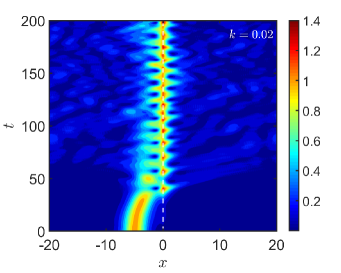
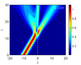
Figure 5: Contour plots showing the evolution of the modulus $|u(x,t)|$ of a nonlocal bright soliton, initially placed at $x_{0}=-5$, with $k=0.02$ (left panel), or placed at $x_{0}=-10$, with $k=0.7$ (right panel); other parameter values are $\epsilon=0.5$ and $d=1$, corresponding to the crossover regime, $\epsilon d\sim 1$. Dashed (white) line depicts the location of the point defect. In the left panel, the slow soliton is trapped at the location of the defect, along with the emission of weak radiation. In the right panel, the fast soliton splits into three parts, a reflected, a transmitted and a trapped one.

4.3 Nonlinear regime, $\epsilon d\ll 1$

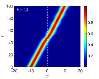
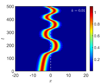
Figure 6: Contour plots showing the evolution of the modulus $|u(x,t)|$ of a nonlocal bright soliton, with $x_{0}=-10$ and $k=0.2$ (left panel), or with $x_{0}=-5$ and $k=0.01$ (right panel); other parameter values are $\epsilon=0.05$ and $d=1$, corresponding to the nonlinear regime, $\epsilon d\ll 1$. Dashed (white) line depicts the location of the point defect. In the left panel, the fast soliton is totally transmitted through the defect, while in the right panel, the slow soliton is trapped from the defect and performs damped oscillations around it.

Next, we consider the nonlinear regime, where the nonlinearity dominates the effect of the impurity, namely $\epsilon d\ll 1$. Essentially, in this case, the fully nonlocal system of Eqs. (5)-(6), can be approximated by a local NLS equation incorporating the defect potential, or a fully nonlocal NLS in the free space.

As in the previously studied regimes, we will investigate the collision of a moving soliton [of the form of Eq. (16)] with the defect, for different values of wavenumber $k$. Since the nonlinear term dominates in this case, one should expect to observe dynamics similar to that found in the context of the local NLS [24, 25, 26]. We find that this is indeed the case, and there exist only two possible outcomes of the soliton-defect collision, namely the scenarios corresponding to $k>\epsilon$ (fast solitons) and $k<\epsilon$ (slow solitons).

Relevant results are shown in Fig. 6 (for $d=1$ and $\epsilon=0.05$), where the left (right) panel depicts the fast (slow) soliton-defect interaction. In the left panel, the soliton is initially located at $x_{0}=-10$, moves towards the defect with $k=0.2$, and is totally transmitted through; it is observed that, in this case, the soliton is only slightly deformed after its transmission through the defect. On the other hand, in the right panel, the slow soliton with $k=0.01$, starts from $x_{0}=-5$, approaches the defect, and gets trapped, performing afterwards an oscillatory motion around the defect. Here, oppositely to the case shown in the left panel of Fig. 5, the oscillations are of moderate amplitude (of the order of the initial soliton-defect distance). Nevertheless, here too, at sufficiently large times, the soliton will eventually be completely captured by the defect trap.

5 Conclusions

Concluding, we have studied the dynamics of nonlocal bright solitons in external potentials. For a specific form of the nonlocal response function —relevant to the evolution of optical beams in thermal media, plasmas and nematic liquid crystals— we have investigated two different cases: (i) external potentials that vary slowly over the soliton scale, and (ii) external potentials in the form of point defects.

Starting from case (i), we have exploited the existence of an exact analytical soliton solution of the model, and developed an analytical approach relying on the analysis of the hydrodynamic form of the nonlocal NLS, and a methodology resembling the adiabatic perturbation theory for solitons. This way, we derived analytical nonlocal soliton solutions in the presence of the potential. These soliton solutions are exact for linear (gravitational-type) potentials, or approximate for smooth potentials of general form. It was shown that the center $X_{0}$ of the nonlocal bright solitons behaves like a particle, obeying the Newtonian equation of motion $\ddot{X_{0}}=-dV/dX_{0}$. Direct numerical simulations were found to be in very good agreement with the analytical predictions. In particular, in the case of the linear potential the soliton evolves without any deformation, following a parabolic trajectory, while in the case of a parabolic trapping potential, the soliton performs harmonic oscillations, of frequency equal to the trap frequency $\Omega$. In the case where the competition between the relevant spatial scales (trap and the soliton’s widths) becomes stronger, we observed that the soliton oscillates featuring a distortion in its shape, but still performs oscillations with a frequency equal to $\Omega$.

In case (ii), we identified three different asymptotic regimes, depending on the relative strength of the defect and the nonlocal nonlinearity. In the case where the defect dominates nonlinearity, it was found that the soliton features wave dynamics, being reflected by or transmitted through the defect, closely following the linear Schrödinger picture. In the case where the defect and the nonlinearity are of equal importance, we found that the problem admits a defect mode — the nonlinear analogue of the bound state of the linear Schrödinger equation. The latter was determined analytically, as a special solution of the hydrodynamic equations pertaining to the nonlocal NLS model, and its existence was validated numerically. In the simulations we observed that the soliton-defect collision may lead to either complete trapping of the soliton by the defect or partial reflection and transmission, again accompanied by partial trapping of the soliton. On the other hand, in the case where the nonlinearity dominates the effect of the impurity, we found a behavior similar to that occurring in the local NLS equation: fast solitons are transmitted through the defect, while slow solitons are captured in the vicinity of the defect, and perform long-lived oscillations around it.

Our analysis, which employs a combination of analytical, asymptotic, and numerical approaches, comes to complement previous work on the local and nonlocal NLS equations. We have introduced an analytical methodology, relying on the analysis of the hydrodynamic form of the nonlocal NLS, which may be used in a variety of relevant problems. This methodology allowed us to shed light on the nonlocality and the external potential scale competition and its concomitant role on the soliton dynamics. Furthermore, it should be pointed out that although the presented results are qualitatively similar to earlier ones corresponding to specific physical settings, they pertain to a broad class of physically relevant nonlocal systems, as mentioned above. Thus, our work offers a rather universal perspective on the particle-wave duality of nonlocal solitons.

It would be interesting to investigate also the dynamics of nonlocal dark solitons in external potentials; this is particularly challenging, as exact dark soliton solutions for the nonlocal NLS model are not available. Furthermore, it would be relevant to generalize our considerations to other localized solitary wave structures (such as vortices) occurring in higher-dimensional settings.

References

- [1] F. Dalfovo, S. Giorgini, L. P. Pitaevskii, and S. Stringari, Rev. Mod. Phys. 71, 463 (1999).
- [2] D. Suter and T. Blasberg, Phys. Rev. A 48, 4583 (1993).
- [3] C. Rotschild, O. Cohen, O. Manela, M. Segev, and T. Carmon, Phys. Rev. Lett. 95, 213904 (2005).
- [4] A. G. Litvak, JETP Lett. 4, 230 (1966).
- [5] A. I. Yakimenko, Y. A. Zaliznyak, and Y. S. Kivshar, Phys. Rev. E 71, 065603(R) (2005).
- [6] M. Peccianti and G. Assanto, Phys. Rep. 516, 147 (2012).
- [7] G. Assanto, Nematicons: Spatial Optical Solitons in Nematic Liquid Crystals (New York, Wiley, 2012).
- [8] T. Lahaye, C. Menotti, L. Santos, M. Lewenstein, and T. Pfau, Rep. Prog. Phys. 72, 126401 (2009).
- [9] Y. S. Kivshar and G. P. Agrawal, Optical solitons: from fibers to photonic crystals (Academic Press, San Diego, 2003).
- [10] L. D. Landau and E. M. Lifschitz, Quantum Mechanics, Non-relativistic theory (Pergamon Press, Oxford, 1965); J. J. Sakurai, Modern Quantum Mechanics (Addison-Wesley, 1994).
- [11] A. M. Kosevich, Physica D 41, 253 (1981).
- [12] M. A. de Moura, J. Phys. A: Math. Gen. 27, 7157 (1994).
- [13] U. Al Khawaja, H. T. C. Stoof, R. G. Hulet, K. E. Strecker, and G. B. Partridge, Phys. Rev. Lett. 89, 200404 (2002).
- [14] C. Hernandez Tenorio, E. V. Vargas, V. N. Serkin, M. Aguero Granados, T. L. Belyaeva, R. P. Moreno, and L. Morales Lara, Quantum Electron. 35, 778 (2005).
- [15] R. Carretero-González, D. J. Frantzeskakis, and P. G. Kevrekidis, Nonlinearity 21, R139 (2008).
- [16] B. Alfassi, C. Rotschild, O. Manela, M. Segev, and D. N. Christodoulides, Opt. Lett. 32, 154 (2007).
- [17] G. Poy, A. J. Hess, A. J. Seracuse, M. Paul, S. Žumer, and I. I. Smalyukh, Nat. Phot. 16 454 (2022).
- [18] M. Peccianti, A. Fratalocchi, and G. Assanto, Opt. Express 26, 6524 (2004).
- [19] F. Kh. Abdullaev and V. A. Brazhnyi, J. Phys. B: At. Mol. Opt. Phys. 45, 085301 (2012).
- [20] Chao-Qing Dai and Jie-Fang Zhang, Nonlinear Dyn. 100, 1621 (2020).
- [21] T. P. Horikis, Eur. Phys. J. Plus 135, 562 (2020).
- [22] Yi-Xiang Chen and Xiao Xiao, Nonlinear Dyn. 109, 2003 (2022).
- [23] The case where the soliton width and the characteristic spatial scale of the potential are of the same order has also been studied for solitons confined in periodic potentials —see, e.g., R. Scharf and A. R. Bishop, Phys. Rev. E 47, 1375 (1993).
- [24] X. D. Cao and B. A. Malomed, Phys. Lett. A 206, 177 (1995).
- [25] R. H. Goodman, P. J. Holmes, and M. I. Weinstein, Physica D 192, 215 (2004).
- [26] J. Holmer, J. Marzuola, and M. Zworski, Commun. Math. Phys. 274, 187 (2007); J. Nonlinear Sci. 17, 349 (2007).
- [27] C. P. Jisha, A. Alberucci, R.-K. Lee, and G. Assanto, Opt. Lett. 36, 1848 (2011).
- [28] M. Peccianti, A. Dyadyusha, M. Kaczmarek, and G. Assanto, Nat. Phys. 2, 737 (2006).
- [29] P. D. Rasmussen, O. Bang, and W. Królikowski, Phys. Rev. E 72, 066611 (2005).
- [30] V. I. Karpman, Sov. Phys. JETP 50, 58 (1979); Phys. Scr. 20, 462 (1979).
- [31] Yu. S. Kivshar and B. A. Malomed, Rev. Mod. Phys. 61, 761 (1989).
- [32] W. Krolikowski, O. Bang, N. I. Nikolov, D. Neshev, J. Wyller, J. J. Rasmussen, and D. Edmundson, J. Opt. B: Quantum Semiclass. Opt. 6, S288 (2004).
- [33] D. Mihalache, Romanian Rep. Phys. 59, 515 (2007).
- [34] B. A. Malomed, Symmetry 14, 1565 (2022).
- [35] G. N. Koutsokostas, T. P. Horikis, P. G. Kevrekidis, and D. J. Frantzeskakis, J. Phys. A: Math. Theor. 54, 085702 (2021).
- [36] W. Krolikowski and O. Bang, Phys. Rev. E 63, 016610 (2001).
- [37] N. I. Nikolov, D. Neshev, O. Bang, and W. Z. Krolikowski, Phys. Rev. E 68, 036614 (2003).