Kinetic Interacting Particle Langevin Monte Carlo

Abstract

This paper introduces and analyses interacting underdamped Langevin algorithms, termed Kinetic Interacting Particle Langevin Monte Carlo (KIPLMC) methods, for statistical inference in latent variable models. We propose a diffusion process that evolves jointly in the space of parameters and latent variables and exploit the fact that the stationary distribution of this diffusion concentrates around the maximum marginal likelihood estimate of the parameters. We then provide two explicit discretisations of this diffusion as practical algorithms to estimate parameters of statistical models. For each algorithm, we obtain nonasymptotic rates of convergence for the case where the joint log-likelihood is strongly concave with respect to latent variables and parameters. In particular, we provide convergence analysis for the diffusion together with the discretisation error, providing convergence rate estimates for the algorithms in Wasserstein-2 distance. To demonstrate the utility of the introduced methodology, we provide numerical experiments that demonstrate the effectiveness of the proposed diffusion for statistical inference and the stability of the numerical integrators utilised for discretisation. Our setting covers a broad number of applications, including unsupervised learning, statistical inference, and inverse problems.

1 Introduction

Parametric latent variable models (LVMs) are ubiquitous in many areas of statistical science, e.g., complex probabilistic models for text, audio, video and images [8, 63, 38] or inverse problems [64]. Intuitively, these models capture the underlying structure of the real data in terms of low-dimensional latent variables - a structure that often exists in real world [67]. However, latent variable models often require nontrivial procedures for maximum likelihood estimation as this quantity is often intractable [25]. Our main aim in this paper is to propose a set of accelerated and stable algorithms for the problem of maximum marginal likelihood estimation in the presence of latent variables and show convergence bounds for them by studying their nonasymptotic behaviour.

Let us consider a generic latent variable model as $p_{\theta}(x,y)$, parameterised by $\theta\in\mathbb{R}^{d_{\theta}}$, for fixed data $y\in{\mathbb{R}}^{d_{y}}$, and latent variables $x\in{\mathbb{R}}^{d_{x}}$. This model is considered for fixed observed data $y$, thus formally we see the statistical model as a real-valued mapping $p_{\theta}(x,y):\mathbb{R}^{d_{x}}\times\mathbb{R}^{d_{\theta}}\to{\mathbb{R}}$. The task we are interested in is to estimate the parameter $\theta$ that explains the fixed dataset $y$. Often, this task is achieved via the maximum likelihood estimation (MLE). In accordance with this, in our setting, due to the presence of latent variables, we aim at finding the maximum marginal likelihood estimate (MMLE) [25], more precisely, our problem takes the form

$$\bar{\theta}_{\star}\in\arg\max_{\theta\in\mathbb{R}^{d_{\theta}}}\log p_{\theta}(y),$$ (1)

where $p_{\theta}(y):=\int p_{\theta}(x,y)\mathrm{d}x$ is the marginal likelihood (also called the model evidence in Bayesian statistics [7]). It is apparent from (1) that the problem cannot be solved via optimisation techniques alone, as the marginal likelihood contains an intractable integral for most statistical models.

Classically, this problem is solved with the iterative Expectation-Maximisation (EM) algorithm [25], which provably converges to a local maximum. This algorithm consists of the E and M steps: (1) the E-step (optimally) produces an estimate for the posterior distribution of latent variables $p_{\theta}(x|y)$ and (2) the M-step maximises the expected log-likelihood estimate w.r.t. the parameter $\theta$. More compactly, starting at $\theta_{0}$, the EM algorithm produces the estimates $(\theta_{n})_{n\in{\mathbb{N}}}$, solving

$$\theta_{n+1}\in\arg\max_{\theta\in{\mathbb{R}}^{d_{\theta}}}\mathbb{E}_{p_{\theta_{n}}(x|y)}[\log p_{\theta}(x,y)].$$

It is easy to establish that $\log p_{\theta_{n+1}}(y)\geq\log p_{\theta_{n}}(y)$, hence the method converges to a local maximum. In this setting, two tasks need to be solved simultaneously: (i) inference, i.e., inferring the distribution of $x$ given $y$ for $\theta_{n}$, in other words, the posterior distribution $p_{\theta_{n}}(x|y)$, (ii) estimation, i.e., estimating the maximiser $\theta_{n+1}$, whose computation requires the inference step. Often, this recursion is impossible to realise, due to two main challenges, namely, the expectation (E) and maximisation (M) steps, which are intractable. These steps can be approximated with a variety of methods, which, due to the simplicity of this algorithm, have been extensively explored. For example, Monte-Carlo EM [66] and stochastic EM [14] have been widely studied, see, e.g., [15, 16, 62, 9, 12, 26].

In the most general case, the EM algorithm is implemented using Markov chain Monte Carlo (MCMC) techniques for the E-step, and numerical optimisation techniques for the M-step, e.g., [50, 48, 46]. With the popularity of unadjusted Langevin methods in Bayesian statistics and machine learning [30, 29, 31, 20, 21, 23], variants of the implementation of expectation-maximisation algorithms using unadjusted chains to perform the E-step have also been proposed. Most notably, [24] studied an algorithm termed SOUL, which performs unadjusted Langevin steps for the E-step and stochastic gradient ascent for the M-step, building on the ideas of [5]. This algorithm required to run a Markov chain for each E-step, resulting in a double-loop algorithm. The bias incurred by unadjusted chains complicates the theoretical analysis and requires a delicate balance of the step-sizes of the Langevin algorithm and gradient step to guarantee convergence [24]. An alternative approach was developed in [45], where instead of running Markov chains to perform E-step, the authors proposed to use an interacting particle system, consisting of $N$ particles. Particle systems, such as the one proposed in [45], are often used to accelerate convergence for gradient-based methods or to replace these entirely ([10, 54, 44, 1, 37] for a review on their advantages and behaviour). In a similar vein, [45] shows that using an algorithm based on an interacting particle system (IPS), termed particle gradient descent (PGD), alleviates the need of running interleaving Markov chains, which can also lead to provable guarantees, see, e.g., [13]. Inspired by the approach in [45], a closely related interacting particle system was proposed in [2], where a properly scaled noise is injected in the $\theta$-dimension. This seemingly small modification is significant, making the algorithm an instance of a Langevin diffusion (an observation we build on in this paper). The authors termed this method interacting particle Langevin algorithm (IPLA) and proved error bounds for the algorithm. In particular, they showed that the parameter-marginal of IPLA iterates, targets a measure of the form $\pi_{\Theta}\propto\exp(-N\log p_{\theta}(y))$, which concentrates around the MMLE estimate with a rate $\mathcal{O}(N^{-1/2})$ where $N$ is the number of particles. The authors of [2] further provided the exponential convergence rate and the discretisation error under the within strongly convex setting. The IPLA methodology has been already utilised in other contexts, see, e.g., [43] for superlinear extensions and [33] for a set of proximal methods based on IPLA, and [3] for relations between IPLA and multiscale methods.

Finally, targeting this sort of measure to solve optimisation problems, is similar to simulated annealing techniques from optimisation (see [35, 40, 28, 41] for a discussion of these methods), which is a commonly proposed approach to MMLE estimation. In particular, [28, 41] consider particle systems and observe sampling improvements in non-convex optimisation, motivating this alternative approach.

Contributions. In this paper, the overdamped Langevin diffusion proposed by [2] is modified by considering the underdamped setting - resulting in another stochastic differential equation (SDE) termed, Kinetic Interacting Particle Langevin Diffusion (KIPLD). In continuous time, our proposed diffusion corresponds to the noisy version of the system proposed in [47], or an acceleration of the overdamped diffusion introduced by [2], see, e.g., [49]. We then propose two underdamped Langevin samplers, which we term Kinetic Interacting Particle Langevin Monte Carlo (KIPLMC), based on this diffusion. Our contributions can be summarised as follows:

• We propose the KIPLD, a diffusion process to optimise the marginal likelihood in latent variable models. Our diffusion process corresponds to $\theta$-noised version of the SDE proposed in [47]. However, in [47], the authors left the problem of nonasymptotic analysis open. In this paper, we provide a nonasymptotic analysis and show that the proposed modification enables us to prove that the stationary measure of this diffusion concentrates around the MMLE (Propositions 1 and 2) and the KIPLD converges to this measure exponentially fast (Proposition 3).

• We propose two discretisations of this diffusion to obtain practical algorithms, which we term Kinetic Interacting Particle Langevin Monte Carlo (KIPLMC) methods. Our first algorithm KIPLMC1 corresponds to a similar discretisation provided by [47] for our diffusion. However, we provide discretisation error bounds for our method, leveraging available results in the literature, showing convergence rates in both time and step-size (Theorem 1). We then introduce a splitting-based explicit discretisation scheme within this setting, which leads to a nontrivial algorithm, which we term KIPLMC2. We provide a nonasymptotic analysis of this method (Theorem 2).

• Finally, we provide numerical results that shows in particular the stability attained by KIPLMC2. We show in particular that this discretisation (which is based on [51]) is more stable than KIPLMC1 and MPGD of [47].

The paper is structured as follows: we present the unadjusted Langevin Algorithm, its underdamped sibling and interacting particle systems for the MMLE problem in the Technical Background, section 2. Following this introduction, we propose a new diffusion for the MMLE problem, the Kinetic Interacting Particle Langevin Diffusion (KIPLD), and present the associated algorithms (KIPLMC1) and (KIPLMC2) in section 3. Finally we identify the convergence rate for the algorithms to the MMLE target with the nonasymptotic analysis of section 4 and make some empirical comparisons in the experiments section 5.

Notation

Denote by $\mathcal{P}(\mathbb{R}^{d})$, for $d\geq 1$, the space of all probability measures over $(\mathbb{R}^{d},\mathcal{B}(\mathbb{R}^{d}))$, where $\mathcal{B}(\mathbb{R}^{d})$ denotes the Borel $\sigma$-algebra over $\mathbb{R}^{d}$. Also consider the Euclidean inner-product space over $\mathbb{R}^{d}$, with inner product $\langle\cdot,\cdot\rangle$ and associated norm $\|\cdot\|$. We will be using this notation interchangeably over different dimensions $d$, assuming that the appropriate inner-product space is chosen. For notational convenience, denote $\{1,\dots,N\}$ as $[N]$ and the set of positive integers as ${\mathbb{N}}$.

Recall that, under a fixed dataset, our model is parameterised over $\theta\in\mathbb{R}^{d_{\theta}}$ and $x\in\mathbb{R}^{d_{x}}$. Let us consider an unnormalised probability model $U(\theta,x)$, where

$$U(\theta,x)=-\log p_{\theta}(x,y).$$

For any $p>0$ define the Wasserstein-$p$ metric as

$$W_{p}(\pi,\nu)=\inf_{\Gamma\in\mathbf{T}(\pi,\nu)}\left(\int\|x-y\|^{p}_{p}\mathrm{d}\Gamma(x,y)\right)^{\frac{1}{p}},$$

where $\mathbf{T}(\pi,\nu)$ denotes the set of couplings over $\mathbb{R}^{d\times d}$, with marginals $\pi$ and $\nu$.

2 Technical Background

Before presenting our proposed diffusion and algorithms, we introduce some concepts that will be useful to us in this paper. In particular, we introduce unadjusted Langevin algorithms, kinetic Langevin Monte Carlo methods, followed by a discussion of the interacting particle Langevin algorithm (IPLA) of [2] for the MMLE problem.

2.1 Unadjusted Langevin Algorithm

Consider the problem of simulating random variables with a law in $\mathcal{P}({\mathbb{R}}^{d})$ of the form

$$\pi({\mathrm{d}}z)\propto e^{-U(z)}{\mathrm{d}}z,$$ (2)

where $U:{\mathbb{R}}^{d}\to{\mathbb{R}}$ is a potential function. This is a classical problem in computational statistics literature, with abundance of Markov chain Monte Carlo (MCMC) methods available, see, e.g., [56] for a book long treatment. In this paper, we focus on a particular class of MCMC algorithm, termed the unadjusted Langevin algorithm (ULA). These methods rely on the fact that the following Langevin diffusion process

$$\mathrm{d}{\mathbf{Z}}_{t}=-\nabla U({\mathbf{Z}}_{t})\mathrm{d}t+\sqrt{2}\mathrm{d}{\mathbf{B}}_{t},$$ (3)

where $({\mathbf{B}}_{t})_{t\geq 0}$ is a standard Brownian motion, leaves the target measure (2) invariant. While this idea is well-known in MCMC literature and exploited for a long time as the proposal of the Metropolis-adjusted Langevin algorithm (MALA) [58, 57, 68], recently several approaches simply drop the Metropolis step in this method and use the plain discretisation of the diffusion (3) as a sampling algorithm. This results in the following discretisation (termed unadjusted Langevin algorithm (ULA) [31, 30] or Langevin Monte Carlo (LMC) [20])

$$Z_{n+1}^{\eta}=Z^{\eta}-\eta\nabla U(Z^{\eta}_{n})+\sqrt{2\eta}W_{n+1}$$

where $(W_{n})_{n\in{\mathbb{N}}}$ are standard $d$-dimensional Normal random variables and $\eta$ corresponds to the step-size of the algorithm.

Sampling with unadjusted Langevin algorithm, for convex $U$, has been extensively studied [30, 23]. The ULA is an efficient way to sample from these distributions, providing exponential convergence to the unique stationary measure and only requiring an un-normalised model. This improved computational performance comes at the expense of inducing a bias of order $\eta^{\frac{1}{2}}$ in the stationary measure of the algorithm [31]. Despite this, the ULA is a natural choice for sampling, as it can be implemented through a variety of discretisations and has, as discussed, favourable theoretical properties (see, [30, 65, 29, 11, 19, 58, 57] and [22], for convergence results under different assumptions on $U$).

2.2 Kinetic Langevin Monte Carlo

An alternative to the Langevin diffusions given in (3), which are generally termed overdamped Langevin diffusions, is another class of Langevin diffusions called underdamped diffusions [53]. This class of diffusions is akin to second-order differential equations and defined over position and momentum variables. The momentum particle’s dynamics are given by Newton’s Law for the motion of a particle, subject to friction and a stochastic forcing, acting as the gradient of the position particle [18]. In particular, the underdamped Langevin diffusion is defined as

$$\mathrm{d}{\mathbf{Z}}_{t} =V_{t}\mathrm{d}t$$ (4)

$$\mathrm{d}{\mathbf{V}}_{t} =-\gamma{\mathbf{V}}_{t}\mathrm{d}t-\nabla_{z}U({\mathbf{Z}}_{t})\mathrm{d}t+\sqrt{2\gamma}\mathrm{d}{\mathbf{B}}_{t},$$

where $\gamma>0$ is called the friction coefficient and $({\mathbf{B}}_{t})_{t\geq 0}$ is a Brownian motion. From this equation, one can recover the overdamped dynamics in (3) by letting $\gamma\to\infty$ and considering the behaviour of the $z$-marginal [52, pg. 58]. Under certain regularity conditions [53], this system is known to be invariant w.r.t. an extended stationary measure of the form

$$\bar{\pi}({\mathrm{d}}z,{\mathrm{d}}v)\propto\exp\left(-U(z)-\frac{1}{2}\|v\|^{2}\right){\mathrm{d}}z{\mathrm{d}}v.$$ (5)

This means that we can recover the samples from our target measure (2) by sampling from (5) where the $z$-marginal of $\bar{\pi}$ is the target measure we would like to sample from.

As the update rules are determined by a numerical approximation of a continuous-time process, how this algorithm performs is dependent on the smoothness of the sample paths and the mixing rate of the system. It is quite easy to see that the sample paths in the underdamped case are smoother, having an Hölder continuity of order $1+\alpha$, for $\alpha\in[0,1/2)$ (see introduction of [23]). Furthermore, similar to the ULA algorithm, this system also has exponentially fast convergence to the stationary measure [23]. By using an underdamped, second-order system, [18] exploit these properties to accelerate the first-order process, connecting this work to Nesterov acceleration and the growing body of literature dedicated to it. Indeed, [18] show that for certain choices of $\gamma$ the underdamped system converges faster to the stationary measure than the overdamped system and identify the regimes in which the underdamped algorithm outperforms the overdamped for their sampling schemes. This acceleration has not only been noted in $W_{2}$, by [23, 17] and others, but also in KL divergence by [49]. The underdamping leads to some interesting properties, such as an “induced regularisation” and more damped momentum effects, as well as, convergence with better dependence on dimension and step-size, as shown in [17]. Hence, the underdamped Langevin diffusion, presents a worthwhile starting point for sampling algorithms and represents a competitive alternative to the popular ULA.

2.3 MMLE via Interacting Particle Langevin Algorithm

These sampling algorithms, however, are not sufficient for parameter estimation, for which we will need to introduce optimisation techniques. As mentioned in the introduction, our main aim in this paper is to develop algorithms to solve the maximum marginal likelihood estimation problem (MMLE). Recall that the MMLE problem is to identify

$$\bar{\theta}_{\star}\in\arg\max_{\theta\in\mathbb{R}^{d_{\theta}}}\log p_{\theta}(y),$$

for fixed $y\in\mathbb{R}^{d_{y}}$ and $p_{\theta}(y)=\int p_{\theta}(x,y){\mathrm{d}}x$. Therefore the MMLE problem is simply the maximisation of an often intractable integral. With the notation $U(\theta,x)=-\log p_{\theta}(x,y)$, the $\theta$-gradient of $\log p_{\theta}(y)$ is given as

$$\nabla_{\theta}\log p_{\theta}(y)=\frac{-\int\nabla_{\theta}U(\theta,x)p_{\theta}(x,y){\mathrm{d}}x}{p_{\theta}(y)}=-\int\nabla_{\theta}U(\theta,x)p_{\theta}(x|y){\mathrm{d}}x,$$ (6)

which is easy to prove (see, e.g., [27, Proposition D.4] and [2, Remark 1]). The expression in (6) is the motivation behind approximate schemes for expectation-maximisation, where one can first sample from $p_{\theta}(x|y)$ for fixed $\theta$ with an MCMC chain and then compute the gradient in (6) with these samples [24, 6]. However, these approaches require non-trivial assumptions on the step-size, as well as having a sample size that may need to grow to ensure that the gradient approximation does not incur asymptotic bias.

In contrast to this approach, [45] propose an IPS, the particle gradient descent (PGD) algorithm, to approximate the gradient of the $\theta$-dynamics by running independent particles to integrate out latent variables. Inspired by this, [2] attempt to solve the MMLE problem with a similar IPS, termed the interacting particle Langevin Algorithm (IPLA), which is a modification of PGD where $\theta$-dynamics contain a carefully scaled noise. This approach produces a system that is akin to an unadjusted Langevin algorithm and makes the theoretical analysis streamlined. The proposed algorithm is a discretisation of a system of interacting Langevin SDEs for the parameter $\theta$ and $N$ particles $X^{1},\dots,X^{N}$. To be precise, the dynamics of $\bm{\theta}_{t}$ and $\bm{X}^{i}_{t}$, for the IPLA, are driven by the system of equations

$$\mathrm{d}\bm{\theta}_{t} =-\frac{1}{N}\sum_{i=1}^{N}\nabla_{\theta}U(\bm{\theta}_{t},{\mathbf{X}}_{t}^{i})\mathrm{d}t+\sqrt{\frac{2}{N}}\mathrm{d}{\mathbf{B}}_{t}^{0},$$ (7)

$$\mathrm{d}{\mathbf{X}}_{t}^{i} =-\nabla_{x}U(\bm{\theta}_{t},{\mathbf{X}}^{i}_{t})\mathrm{d}t+\sqrt{2}\mathrm{d}{\mathbf{B}}_{t}^{i},\qquad\text{for }i\in[N].$$ (8)

where $({\mathbf{B}}_{t}^{0})_{t\geq 0}$ is a Brownian motion evolving on ${\mathbb{R}}^{d_{\theta}}$ and $({\mathbf{B}}_{t}^{i})_{t\geq 0}$ for $i\in[N]$ are Brownian motions evolving on $\mathbb{R}^{d_{x}}$. It is quite easy to note that the drift term for the $\theta$-dynamics can be seen as the empirical approximation of the “true” drift (6) with $N$ particles drawn from a measure drifting towards $p_{\theta}(x|y)$. In this case, [2] observe that the stationary measure of this system is given as

$$\pi^{N}({\mathrm{d}}\theta,{\mathrm{d}}x_{1},\dots,{\mathrm{d}}x_{N})\propto\exp\left(-\sum_{i=1}^{N}U(\theta,x_{i})\right){\mathrm{d}}\theta{\mathrm{d}}x_{1}\dots\mathrm{d}x_{N}.$$

It is easy to show that, the $\theta$-marginal of this measure concentrates on the MMLE $\bar{\theta}_{\star}$ as $N$ grows, similar to annealing techniques developed in traditional optimisation [39]. The authors of [2] identify the convergence rate to the joint stationary measure, as well as, an error bound for the discretisation error, from which an error can be determined between the $\theta$-iterate of the algorithm and the MMLE. With this nonasymptotic analysis, [2] identify parameters needed to implement the algorithm and introduce an order of convergence guarantee in $W_{2}$. The algorithm is empirically shown to be competitive with state-of-the-art models, such as SOUL [24] and the PGD proposed in [45]. Further, the IPLA algorithm lays the foundation for many avenues for further exploration: such as considering a kinetic Langevin algorithm and considering other numerical discretisations of proposed SDEs as we will do in this paper.

3 Kinetic Interacting Particle Langevin Monte Carlo

Recall that our goal is to combine the advantages of underdamped Langevin diffusions with the interacting particle systems proposed by [2, 45, 47], to estimate the MMLE $\bar{\theta}_{\star}$. In this section we present a diffusion and two algorithms to this end. Indeed, this diffusion will be an underdamped version of the system of overdamped Langevin diffusions of the IPLA algorithm (7).

3.1 Kinetic Interacting Particle Langevin Diffusion

We introduce the KIPLD system, the diffusion obtained by replacing the overdamped dynamics of the IPLA with underdamped ones. This is given by

$$\mathrm{d}\bm{\theta}_{t} ={\mathbf{V}}^{\theta}_{t}\mathrm{d}t$$

$$\mathrm{d}{\mathbf{X}}^{i}_{t} ={\mathbf{V}}^{x_{i}}_{t}\mathrm{d}t,$$ (KIPLD)

$$\mathrm{d}{\mathbf{V}}^{\theta}_{t} =-\gamma{\mathbf{V}}^{\theta}_{t}\mathrm{d}t-\frac{1}{N}\sum_{i=1}^{N}\nabla_{\theta}U(\bm{\theta}_{t},{\mathbf{X}}^{i}_{t})\mathrm{d}t+\sqrt{\frac{2\gamma}{N}}\mathrm{d}{\mathbf{B}}^{0}_{t}$$

$$\mathrm{d}{\mathbf{V}}^{x_{i}}_{t} =-\gamma{\mathbf{V}}_{t}^{x_{i}}\mathrm{d}t-\nabla_{x}U(\bm{\theta}_{t},{\mathbf{X}}_{t}^{i})\mathrm{d}t+\sqrt{2\gamma}\mathrm{d}{\mathbf{B}}_{t}^{i},\qquad\text{for }i\in[N]$$

where $({\mathbf{B}}_{t}^{i})_{t\geq 0}$ for $i\in[N]$ is a family of ${\mathbb{R}}^{d_{x}}$-valued Brownian motions and $({\mathbf{B}}_{t}^{0})_{t\geq 0}$ is an $\mathbb{R}^{d_{\theta}}$-valued Brownian motion. For notational convenience we will say that the particles and momenta have combined dimension of $d_{z}=d_{\theta}+Nd_{x}$ each. Similarly to the algorithm proposed by [2], we have a system of $N$ particles for the empirical approximation of latent variable distribution. This system corresponds to relaxing the limit on $\gamma$, the “friction” parameter, for the algorithm proposed by [2]. Adding the friction hyper-parameter $\gamma$ should allow for improved regularisation and dampening momentum effects, as discussed in [49]. We will note some of this behaviour in the experimental section, where the momentum effect can be observed and tuned to produce optimal convergence behaviour.

An alternative perspective is that, in line with the work done by [2], we consider here an analogue of the momentum particle gradient descent (MPGD) scheme [47] with noise. In particular, we are injecting the $\theta$-dynamics with the appropriately scaled $\sqrt{2/N}{\mathrm{d}}{\mathbf{B}}^{0}_{t}$. The advantage of studying this analogue emerges in the numerous results available for Langevin diffusions of kinetic-type, as well as allowing us to recover the algorithm proposed by [47] by considering this version as a noised version of the MPGD (indeed for large $N$, this difference should be more attenuated). However, in contrast to [47], we set both the friction parameters $\gamma$ for the $\theta$ and $x$ dynamics to be the same. The results presented here should naturally extend to other cases.

3.2 Kinetic Interacting Particle Langevin Monte Carlo Methods

We now introduce two numerical integrators for the KIPLD: firstly, we consider an Exponential Integrator, as discussed in [23]; secondly, the Splitting scheme is applied, as described in [51]. These algorithms for kinetic Langevin samplers have two parameters, namely, the step-size $\eta>0$, which assumed to be small, and the friction coefficient $\gamma>0$, determining momentum effects.

3.2.1 Exponential Integrator (KIPLMC1)

[18] introduce a variant of the Hamiltonian Monte Carlo, the KLMC, which has improved convergence rate when compared to the Langevin MCMC proposed by [31]: having $W_{2}$ error of order $\mathcal{O}(n^{-1})$, for step-count $n$, rather than $\mathcal{O}(n^{-\frac{1}{2}})$ [18, Thm. 1]. This method is proposed for sampling from underdamped Langevin diffusions, as, unlike Euler-Maruyama, this approach seems able to exploit the higher order of convergence of the underlying process [23]. The bounds on the convergence rate for this algorithm are further improved in [23], who tighten the bound with respect to the condition number $L/\mu$ and improve sensitivity to the initial choice is reduced. On top of this, [23] identify the cases in which the KLMC outperforms Langevin MCMC, based on the bounds established for the the two algorithms. In particular, when $dn$ is large relative to $L$ the KLMC is preferable to the Langevin MCMC. Here $d$ denotes the dimension of the SDE system and $n$ the total step-count.

Motivated by this we seek to apply this scheme to the diffusion KIPLD and seek to recover favourable results. Following [23], we begin by defining recursively,

$$\psi_{0}(t) =e^{-\gamma t}$$

$$\psi_{1}(t) =\int_{0}^{t}e^{-\gamma s}{\mathrm{d}}s=\frac{1}{\gamma}(e^{-\gamma t}-1)$$

$$\psi_{2}(t) =\frac{1}{\gamma}\int_{0}^{t}(e^{-\gamma s}-1){\mathrm{d}}s=\frac{1}{\gamma^{2}}(e^{-\gamma t}-1)-\frac{t}{\gamma}.$$

These terms emerge from the Itô formula used to estimate the expectations and their covariances (see Lemma 11 [18] for a full derivation). The pairs $\varepsilon_{n}^{i}$, $\varepsilon_{n}^{i,\prime}$, for $i\in[N]$, are i.i.d. standard normal Gaussians with pair-wise covariance matrix

$$C=\int_{0}^{\eta}\begin{pmatrix}\psi_{0}(t)^{2}&\psi_{0}(t)\psi_{1}(t)\\ \psi_{0}(t)\psi_{1}(t)&\psi_{1}(t)^{2}\end{pmatrix}\mathrm{d}t.$$ (9)

This covariance matrix is the covariance between the dynamics of the position particle and the momentum particle, as shown in [18, Lemma 11].

The scheme is recovered by updating the particle positions with the expectations of the particles conditioned on the previous time-step and adding Gaussian noise with covariance $C$. Thus, the scheme produces the same first and second momenta as the diffusion we seek to target. Formally, the scheme is given by

$$\theta_{n+1} =\theta_{n}+\psi_{1}(\eta)V^{\theta}_{n}-\frac{\psi_{2}(\eta)}{N}\sum_{i=1}^{N}\nabla_{\theta}U(\theta_{n},X^{i}_{n})+\sqrt{\frac{2\gamma}{N}}\varepsilon^{0,\prime}_{n+1}$$ (KIPLMC1)

$$X^{i}_{n+1} =X^{i}_{n}+\psi_{1}(\eta)V^{x_{i}}_{n}-\psi_{2}(\eta)\nabla_{x}U(\theta_{n},X^{i}_{n})+\sqrt{2\gamma}\varepsilon_{n+1}^{i,\prime}$$

$$V^{\theta}_{n+1} =\psi_{0}(\eta)V^{\theta}_{n}-\frac{\psi_{1}(\eta)}{N}\sum_{i=1}^{N}\nabla_{\theta}U(\theta_{n},X^{i}_{n})+\sqrt{\frac{2\gamma}{N}}\varepsilon^{0}_{n+1}$$

$$V^{x_{i}}_{n+1} =\psi_{0}(\eta)V^{x_{i}}_{n}-\psi_{1}(\eta)\nabla_{x}U(\theta_{n},X^{i}_{n})+\sqrt{2\gamma}\varepsilon^{i}_{n+1}$$

for $i\in[N]$, where $\varepsilon_{n}$ and $\varepsilon^{\prime}_{n}$ are standard Gaussians with pairwise covariance given by $C$. The scheme converges for certain choices of $\eta$, depending on the assumptions set on $U$. The full algorithm is given in Algorithm 1.

Algorithm 1 KIPLMC1 Algorithm

$\gamma,\eta>0$, $N,K\in{\mathbb{N}}$

Draw $\theta_{0},X^{i}_{0},V^{\theta}_{0},V^{x_{i}}_{0}$, for $i\in[N]$

for $n=0:K-1$ do

     Draw $\varepsilon_{n},\varepsilon^{\prime}_{n}$ from $d_{\theta}+Nd_{x}$-dimensional Gaussians with covariance $C$ given in (9)

     $\theta_{n+1}=\theta_{n}+\psi_{1}(\eta)V^{\theta}_{n}-\frac{\psi_{2}(\eta)}{N}\sum_{i=1}^{N}\nabla_{\theta}U(\theta_{n},X^{i}_{n})+\sqrt{\frac{2\gamma}{N}}\varepsilon^{0,\prime}_{n+1}$

     $X^{i}_{n+1}=X^{i}_{n}+\psi_{1}(\eta)V^{x_{i}}_{n}-\psi_{2}(\eta)\nabla_{x}U(\theta_{n},X^{i}_{n})+\sqrt{2\gamma}\varepsilon_{n+1}^{i,\prime}$

     $V^{\theta}_{n+1}=\psi_{0}(\eta)V^{\theta}_{n}-\frac{\psi_{1}(\eta)}{N}\sum_{i=1}^{N}\nabla_{\theta}U(\theta_{n},X^{i}_{n})+\sqrt{\frac{2\gamma}{N}}\varepsilon^{0}_{n+1}$

     $V^{x_{i}}_{n+1}=\psi_{0}(\eta)V^{x_{i}}_{n}-\psi_{1}(\eta)\nabla_{x}U(\theta_{n},X^{i}_{n})+\sqrt{2\gamma}\varepsilon^{i}_{n+1}$

     for $i\in[N]$ return $\theta_{K}$

3.2.2 A Splitting Scheme (KIPLMC2)

The KIPLMC splitting algorithm (KIPLMC2) is an adaptation of the underdamped Langevin sampler introduced by [51], based on classic splitting techniques from MCMC. Specifically, [51] propose an OBABO scheme as the discretisation scheme, which is a second order scheme only requiring the computation of $\nabla U$. The idea is to split the numerical scheme into individually solveable components. In our underdamped case (KIPLD), we have: (A) the update of $\theta$ and $X^{i}$ with known $V^{\theta}$ and $V^{x_{i}}$; (B) update $V^{\theta}$ and $V^{x_{i}}$ with $\frac{1}{N}\sum_{i=1}^{N}\nabla_{\theta}U(\theta,X^{i})$ and $\nabla_{x_{i}}U(\theta,X^{i})$ as gradients respectively; (O) solve the Ornstein-Uhlenbeck equation with the terms $V^{\theta}$ and $V^{x_{i}}$. Thus, the algorithm “splits” the equation into components with known solutions. The order in which these steps are taken is critical and in our case we will limit ourselves to considering the OBABO scheme from [51].

In our case we introduce the KIPLMC2 algorithm based on the OBABO scheme, given as

$$\theta_{n+1} =\theta_{n}+\eta(\delta V_{n}^{\theta}+\frac{1}{\sqrt{N}}\sqrt{1-\delta^{2}}\varepsilon_{n+1}^{0})-\frac{\eta^{2}}{2N}\sum_{i=1}^{N}\nabla_{\theta}U(\theta_{n},X_{n}^{i})$$

$$X^{i}_{n+1} =X^{i}_{n}+\eta(\delta V_{n}^{x_{i}}+\sqrt{1-\delta^{2}}\varepsilon_{n+1}^{i})-\frac{\eta^{2}}{2}\nabla_{x}U(\theta_{n},X_{n}^{i})$$ (KIPLMC2)

$$V^{\theta}_{n+1} =\delta^{2}V_{n}^{\theta}-\frac{\delta\eta}{2}\left(\frac{1}{N}\sum_{i=1}^{N}\nabla_{\theta}U(\theta_{n},X_{n}^{i})+\frac{1}{N}\sum_{i=1}^{N}\nabla U(\theta_{n+1},X^{i}_{n+1})\right)+\frac{1}{\sqrt{N}}\sqrt{1-\delta^{2}}(\delta\varepsilon^{0}_{n+1}-\varepsilon_{n+1}^{0,\prime})$$

$$V^{x_{i}}_{n+1} =\delta^{2}V_{n}^{x_{i}}-\frac{\delta\eta}{2}(\nabla_{x}U(\theta_{n},X^{i}_{n})+\nabla_{x}U(\theta_{n+1},X^{i}_{n+1}))+\sqrt{1-\delta^{2}}(\delta\varepsilon^{i}_{n+1}+\varepsilon^{i,\prime}_{n+1})$$

for $i\in[N]$, where $\delta=e^{-\eta\gamma/2}$ and in this case $\varepsilon^{i}$ and $\varepsilon^{i,\prime}$ are i.i.d. standard Gaussians in this case. The full algorithm is given in Algorithm 2.

Algorithm 2 KIPLMC1 Algorithm

$\gamma,\eta>0$, $N,K\in{\mathbb{N}}$

Draw $\theta_{0},X^{i}_{0},V^{\theta}_{0},V^{x_{i}}_{0}$, for $i\in[N]$

for $n=0:K-1$ do

     Draw $\varepsilon_{n},\varepsilon^{\prime}_{n}$ from $d_{\theta}+Nd_{x}$-dimensional Gaussians

     (O+B)

     $V^{\theta}_{n+\frac{1}{2}}=\delta V^{\theta}_{n}+\frac{1}{\sqrt{N}}\sqrt{1-\delta^{2}}\varepsilon^{0}_{n+1}-\frac{\eta}{2N}\sum_{i=1}^{N}\nabla_{\theta}U(\theta_{n},X_{n}^{i})$

     $V^{x_{i}}_{n+\frac{1}{2}}=\delta V^{x_{i}}_{n}+\sqrt{1-\delta^{2}}\varepsilon^{i}_{n+1}-\eta\nabla_{x}U(\theta_{n},X_{n}^{i})$

     (A)

     $\theta_{n+1}=\theta_{n}+\eta V^{\theta}_{n+\frac{1}{2}}$

     $X^{i}_{n+1}=X^{i}_{n}+\eta V^{x_{i}}_{n+\frac{1}{2}}$

     (B+O)

     $V^{\theta}_{n+1}=\delta(V^{\theta}_{n+\frac{1}{2}}-\frac{\eta}{2N}\sum_{i=1}^{N}\nabla_{\theta}U(\theta_{n+1},X_{n+1}^{i})+\frac{1}{\sqrt{N}}\sqrt{1-\delta^{2}}\varepsilon^{0,\prime}_{n+1}$

     $V^{x_{i}}_{n+1}=\delta(V^{x_{i}}_{n+\frac{1}{2}}-\frac{\eta^{2}}{2}\nabla_{x}U(\theta_{n+1},X^{i}_{n+1})+\frac{1}{\sqrt{N}}\sqrt{1-\delta^{2}}\varepsilon^{0,\prime}_{n+1}$ return $\theta_{K}$

To understand where this system comes from, observe that the (O) and (B) steps produce a half update of $V^{\theta}$ and $V^{x_{i}}$. Note that the first two summands in both equations form the (O) step and the last term the (B) step. With these estimates $\theta$ and $X^{i}$ are updated: the (A) step. Following this the (O) and (B) steps are performed in reverse order, using the updated $\theta_{n+1}$, $X^{i}_{n+1}$ and the half-step value of $V^{\theta}_{n+\frac{1}{2}}$ and $V^{x_{i}}_{n+\frac{1}{2}}$. Giving us the desirable property of being a second-order, explicit scheme, which does not require computation of $\nabla^{2}U$.

4 Nonasymptotic Analysis

In this section, we provide the convergence results for both the analytic and numerical schemes in the nonasymptotic regime of $\gamma<\infty$. In Section 4.3, we identify the stationary measure for KIPLD and show an exponential convergence rate to it, as well as, its concentration onto the MMLE solution $\bar{\theta}_{\star}$ as $N$ grows. Following this, in Section 4.3.2, the error bounds for the two algorithms are introduced, thus allowing us to identify the convergence rate of KIPLMC1 and KIPLMC2 to the MMLE solution $\bar{\theta}_{\star}$.

4.1 Assumptions

We first lay out our assumptions to prove the convergence of the numerical schemes outlined in 3. Our assumptions are generic, i.e., we merely assume strong convexity and $L$-Lipschitz gradients for the potential $U$. These assumptions are akin to the assumptions made in [31, 22] for the unadjusted Langevin algorithm. As such, the assumptions are necessary for basic building blocks of the theory - but it is possible to relax them, as can be seen in [69, 4].

We start with the following assumptions on the potential $U$.

H1.

Let $z,z^{\prime}\in\mathbb{R}^{d_{\theta}+d_{x}}$, we suppose that there exists a $\mu$ s.t.

$$\langle z-z^{\prime},\nabla U(z)-\nabla U(z^{\prime})\rangle\geq\mu\|z-z^{\prime}\|^{2}.$$

This assumption also implies that $\nabla^{2}U$ is positive definite, i.e., $\nabla^{2}U(z)\succeq\mu I$ for all $z\in\mathbb{R}^{d_{\theta}+d_{x}}$.

H2.

We suppose $U\in\mathcal{C}^{1}$ and for any $z,z^{\prime}\in\mathbb{R}^{d_{\theta}+d_{x}}$ there exists a constant $L>0$ s.t.

$$\|\nabla U(z)-\nabla U(z^{\prime})\|\leq L\|z-z^{\prime}\|.$$

4.2 The proof strategy

Given the assumptions above, we aim at bounding the optimisation error of the numerical schemes, i.e., the difference between the law of the numerical scheme and the optimal MMLE solution $\bar{\theta}_{\star}$. Let $(\theta_{n})_{n\geq 0}$ be the sequence of iterates generated by a numerical scheme, for example, KIPLMC1 or KIPLMC2. Finally, let $\pi_{\Theta}$ denote the $\theta$-marginal of the stationary measure of the diffusion KIPLD, and $\delta_{\bar{\theta}_{\star}}$ denote the Dirac measure at $\bar{\theta}_{\star}$. We denote the law of $\theta_{n}$ by $\mathcal{L}(\theta_{n})$. The optimisation error is then defined as ${\mathbb{E}}[\|\theta_{n}-\bar{\theta}_{\star}\|^{2}]^{1/2}$.

In order to proceed, we first note that ${\mathbb{E}}[\|\theta_{n}-\bar{\theta}_{\star}\|^{2}]^{1/2}=W_{2}(\mathcal{L}(\theta_{n}),\delta_{\bar{\theta}_{\star}})$, where $\mathcal{L}(\theta_{n})$ denotes the law of $\theta_{n}$. This is due to the fact that the set of couplings between a measure $\nu$ and another measure $\delta_{y}$ contains a single element $\delta_{y}\otimes\nu$ [59, Section 1.4], thus the infimum in $W_{2}$ is attained by the coupling $\delta_{\bar{\theta}_{\star}}\otimes\mathcal{L}(\theta_{n})$. Using this, we can then write

$${\mathbb{E}}[\|\theta_{n}-\bar{\theta}_{\star}\|^{2}]^{1/2} =W_{2}(\mathcal{L}(\theta_{n}),\delta_{\bar{\theta}_{\star}})$$

$$\leq\underbrace{W_{2}(\pi_{\Theta},\delta_{\bar{\theta}_{\star}})}_{\textnormal{concentration}}+\underbrace{W_{2}(\mathcal{L}(\theta_{n}),\pi_{\Theta})}_{\textnormal{convergence}},$$ (10)

using the triangle inequality as the Wasserstein distance is a metric. The first term in the right-hand side of (10) is the concentration of the stationary measure $\pi_{\Theta}$ onto the MMLE solution $\bar{\theta}_{\star}$, which is given by Proposition 2 below. The second term is the convergence of the numerical scheme to the stationary measure $\pi_{\Theta}$ which will be proved for each scheme separately.

4.3 Nonasymptotic convergence bounds

As outlined above in (10), we will first show the concentration of the stationary measure $\pi_{\Theta}$ onto the MMLE solution $\bar{\theta}_{\star}$. We then show the convergence of the numerical schemes to the stationary measure $\pi_{\Theta}$. Finally, we will provide the error bounds for the numerical schemes.

4.3.1 Concentration of the stationary measure

We are interested in the behaviour of the stationary measure of KIPLD. This is a non-standard underdamped Langevin diffusion, thus, we need to first identify the stationary measure of the system. Recall that we are only interested in $\theta$-marginal of this stationary measure and we denote it by $\pi_{\Theta}$. We first have the following proposition.

Proposition 1.

Let $\pi_{\Theta}$ be the $\theta$-marginal of the stationary measure of the KIPLD. Then, we can write its density as

$$\pi_{\Theta}(\theta)\propto\exp(-N\kappa(\theta)).$$ (11)

where $\kappa(\theta)=-\log p_{\theta}(y)$.

Proof.

See Appendix B.1. $\Box$

This result shows that the KIPLD targets the right object: As $N$ grows, $\pi_{\Theta}$ will concentrate on the minimisers of $\kappa(\theta)$ by a classical result [39]. This shows that the number of particles $N$ acts as an inverse temperature parameter in the underdamped diffusion. Since the minimiser of $\kappa(\theta)$ is the maximiser of $\log p_{\theta}(y)$, we can see that the stationary measure of the KIPLD is concentrating on the MMLE solution $\bar{\theta}_{\star}$. In particular, under the assumption H1, we have the following nonasymptotic concentration result.

Proposition 2.

Under H1, the function $\theta\mapsto\log p_{\theta}(y)$ is $\mu$-strongly log concave. Furthermore, we have

$$W_{2}(\pi_{\Theta},\delta_{\bar{\theta}_{\star}})\leq\sqrt{\frac{2d_{\theta}}{\mu N}},$$

where $\bar{\theta}_{\star}=\arg\max_{\theta\in\Theta}\log p_{\theta}(y)$, which is unique.

Proof.

See Appendix B.2. $\Box$

This shows that there is an explicit rate of convergence of the $\theta$-marginal of the stationary measure of KIPLD to the MMLE solution $\bar{\theta}_{\star}$. This is a key result, as it shows that the stationary measure of the system is concentrating on the MMLE solution as $N$ grows. We note that such results are also potentially possible under nonconvex settings [69, 4].

4.3.2 Convergence of the KIPLD to the stationary measure

We next demonstrate that the KIPLD converges to its stationary measure $\pi_{\Theta}$ exponentially fast in the strongly log-concave case. Indeed, knowing that the system KIPLD is ergodic, we would like to quantify the rate at which this mixing occurs, specifically at what rate the $W_{2}$ distance of the process and its stationary distribution converges for a possibly large range of $\gamma$.

Proposition 3.

Let $(\bm{\theta}_{t})_{t\geq 0}$ and $(\bm{\theta}^{\prime}_{t})_{t\geq 0}$ be $\theta$-marginals of two solutions of the KIPLD SDE, initialised at $\nu\otimes\mathcal{N}(0,\mathbb{I}_{d_{z}})$ and $\nu^{\prime}\otimes\mathcal{N}(0,\mathbb{I}_{d_{z}})$ respectively. Then under H1 and H2 and for $\gamma\geq\sqrt{\mu+L}$, we have

$$W_{2}(\mathcal{L}(\bm{\theta}_{t}),\mathcal{L}(\bm{\theta}^{\prime}_{t}))\leq\sqrt{2}\exp\left(-\frac{\mu}{\gamma}t\right)\mathbb{E}[\|{\mathbf{Z}}_{0}-{\mathbf{Z}}_{0}^{\prime}\|^{2}]^{1/2}.$$

where ${\mathbf{Z}}_{0}^{i}=N^{-1/2}{\mathbf{X}}_{0}^{i}$ for $i\in[N]$, ${\mathbf{Z}}_{0}=(\bm{\theta}_{0},{\mathbf{Z}}_{0}^{1},\ldots,{\mathbf{Z}}_{0}^{N})^{\top}\in{\mathbb{R}}^{d_{\theta}+Nd_{x}}$ and similarly for ${\mathbf{Z}}_{0}^{\prime}$. ${\mathbf{Z}}_{0}\sim\nu$ and ${\mathbf{Z}}_{0}^{\prime}\sim\nu^{\prime}$, where $\nu,\nu^{\prime}\in\mathcal{P}(\mathbb{R}^{d_{z}})$ with bounded second moments.

Proof.

See Appendix B.3. $\Box$

This proposition shows that, under the conditions expressed in Prop. 3, the KIPLD SDE defines a contraction.

4.3.3 Nonasymptotic analysis of KIPLMC1

In this section we present our first main result showing the convergence rate of KIPLMC1. The result is provided in the following theorem.

Theorem 1.

Let $(\theta_{n})_{n\in{\mathbb{N}}}$ be the iterates of KIPLMC1 and suppose that the process is initialised as $(Z_{0},V^{z}_{0})^{T}\sim\nu\otimes\mathcal{N}(0,\mathbb{I}_{d_{z}})$, where $\nu\in\mathcal{P}(\mathbb{R}^{d_{z}})$ has bounded second moments. Under Assumptions H1 and H2 and with $\gamma\geq\sqrt{\mu+L}$ and $\eta\leq\mu/(4\gamma L)$, we have

$${\mathbb{E}}[\|\theta_{n}-\bar{\theta}_{\star}\|^{2}]^{1/2}\leq\sqrt{2}\left(1-\frac{3\mu\eta}{4\gamma}\right)^{n}{\mathbb{E}}[\|Z_{0}-\bar{Z}_{\star}\|^{2}]^{1/2}+\sqrt{2}\frac{L\eta}{\mu}\sqrt{\frac{d_{\theta}+Nd_{x}}{N}}+\sqrt{\frac{2d_{\theta}}{\mu N}},$$

where $Z_{0}=(\theta_{0},N^{-1/2}X^{1}_{0},\dots,N^{-1/2}X^{N}_{0})^{\intercal}$, the initialisation step of the KIPLMC1 where $\bar{Z}_{\star}\sim\tilde{\pi}$ and $\tilde{\pi}$ is the extended target measure described in Lemma A.3.

Proof.

See Appendix B.4. $\Box$

The result follows from the fact that the target measure $\pi_{\Theta}$ of our system concentrates on the maximiser which is given by Proposition 2 and using the results in [23] for kinetic Langevin diffusions and the exponential integrator discretisation. Further, we replicate the choice made in [23] of initialising the momentum particle according to $\mathcal{N}(0,\mathbb{I}_{d_{z}})$, the stationary measure under the momentum marginal.

4.3.4 Nonasymptotic analysis of KIPLMC2

In the following section, we present our second main result, showing the convergence rate of KIPLMC2. The rate is explicitly given in the subsequent theorem.

Theorem 2.

Let $(\theta_{n})_{n\in\mathbb{N}}$ be the iterates of KIPLMC2 and suppose that the process is initialised as $(Z_{0},V^{z}_{0})^{T}\sim\nu\otimes\mathcal{N}(0,\mathbb{I}_{d_{z}})$, where $\nu\in\mathcal{P}(\mathbb{R}^{d_{z}})$ has bounded second moments. Under Assumptions H1 and H2 and with $\gamma\geq 2\sqrt{L}$ and $\eta\leq\frac{\mu}{33\gamma^{3}}$, we have

$${\mathbb{E}}[\|\theta_{n}-\bar{\theta}_{\star}\|^{2}]^{1/2}\leq C\left(\left(1-\frac{\eta\mu}{3\gamma}\right)^{\frac{n}{2}}\mathbb{E}[\|Z_{0}-Z^{\star}\|^{2}]^{1/2}+\eta\sqrt{2d_{z}}\frac{6\gamma K}{\mu}\right)+\sqrt{\frac{2d_{\theta}}{\mu N}},$$

where $Z_{0}=(\theta_{0},N^{-1/2}X^{1}_{0},\dots,N^{-1/2}X^{N}_{0})^{\intercal}$, the initialisation step of the KIPLMC2, $\bar{Z}_{\star}\sim\tilde{\pi}$ and $\tilde{\pi}$ is the extended target measure described in Lemma A.3. The constants $C$ and $K$ are given as

$$C=\sqrt{3}(\sqrt{L}\lor\sqrt{L}^{-1}),\qquad K=L\left(1+e^{L\eta^{2}}\left(\frac{\eta}{6}+\frac{\eta^{2}L}{24}\right)\right)\left(1+\frac{\eta L}{2\sqrt{\mu}}\right).$$

Note $K$ converges to $L$ as $\eta\to 0$.

Proof.

See Appendix B.5. $\Box$

This is again is a simple application of the triangle inequality for the concentration of $\pi_{\Theta}$ from Proposition 2 and the convergence results for kinetic Langevin diffusions approximated by a second-order splitting scheme from [51].

5 Experiments

In the following section a comparison will be made between the empirical results of KIPLMC1, KIPLMC2 algorithms, as well as, that of MPGD from [47]. Specifically, we consider a Bayesian logistic regression LVM for which one can discuss our assumptions in detail.

5.1 Bayesian Logistic Regression on Synthetic Data

We follow the experimental setting in [45] and [2] and start with comparisons between algorithms on a synthetic dataset for which we know the true solution. More precisely, consider the Bayesian logistic regression model

$$p_{\theta}(x)=\mathcal{N}(x;\theta,\sigma^{2}I_{d_{x}}),\qquad p(y|x)=\prod_{j=1}^{d_{y}}s(v_{j}^{\intercal}x)^{y_{j}}(1-s(v_{j}^{\intercal}x))^{1-y_{j}}.$$

Here $s(u)=e^{u}/(1+e^{u})$ is the logistic function and $v_{j}$, $j\in[d_{y}]$ are the set of $d_{x}$-dimensional covariates with corresponding responses $y_{j}\in\{0,1\}$. $\sigma$ is given and fixed throughout. We generate a synthetic set of covariates, $\{v_{j}\}_{j=1}^{d_{y}}\subset\mathbb{R}^{d_{x}}$, from which are simulated a synthetic set of observations $y_{j}|\bar{\theta}_{\star},x,v_{j}$, for fixed $\bar{\theta}_{\star}$, via a Bernoulli random variable with probability $s(v_{j}^{\intercal}x)$. The algorithm is tested on the recovery of this value of $\bar{\theta}_{\star}$.

The marginal likelihood is given as,

$$p_{\theta}(y)=\frac{1}{(2\pi\sigma^{2})^{d_{x}/2}}\int_{\mathbb{R}^{d_{x}}}\left(\prod_{j=1}^{d_{y}}s(v_{j}^{\intercal}x)^{y_{j}}(1-s(v_{j}^{\intercal}x))^{1-y_{j}}\right)\exp\left(\frac{-\|x-\theta\|^{2}}{2\sigma^{2}}\right)\mathrm{d}x.$$

From this it easy to see that the gradients of $U$ are given as,

$$\nabla_{\theta}U(\theta,x)=-\frac{x-\theta}{\sigma^{2}},\qquad\nabla_{x}U(\theta,x)=\frac{x-\theta}{\sigma^{2}}-\sum_{j=1}^{d_{y}}(y_{j}-s(v_{j}^{\intercal}x))v_{j}.$$ (12)

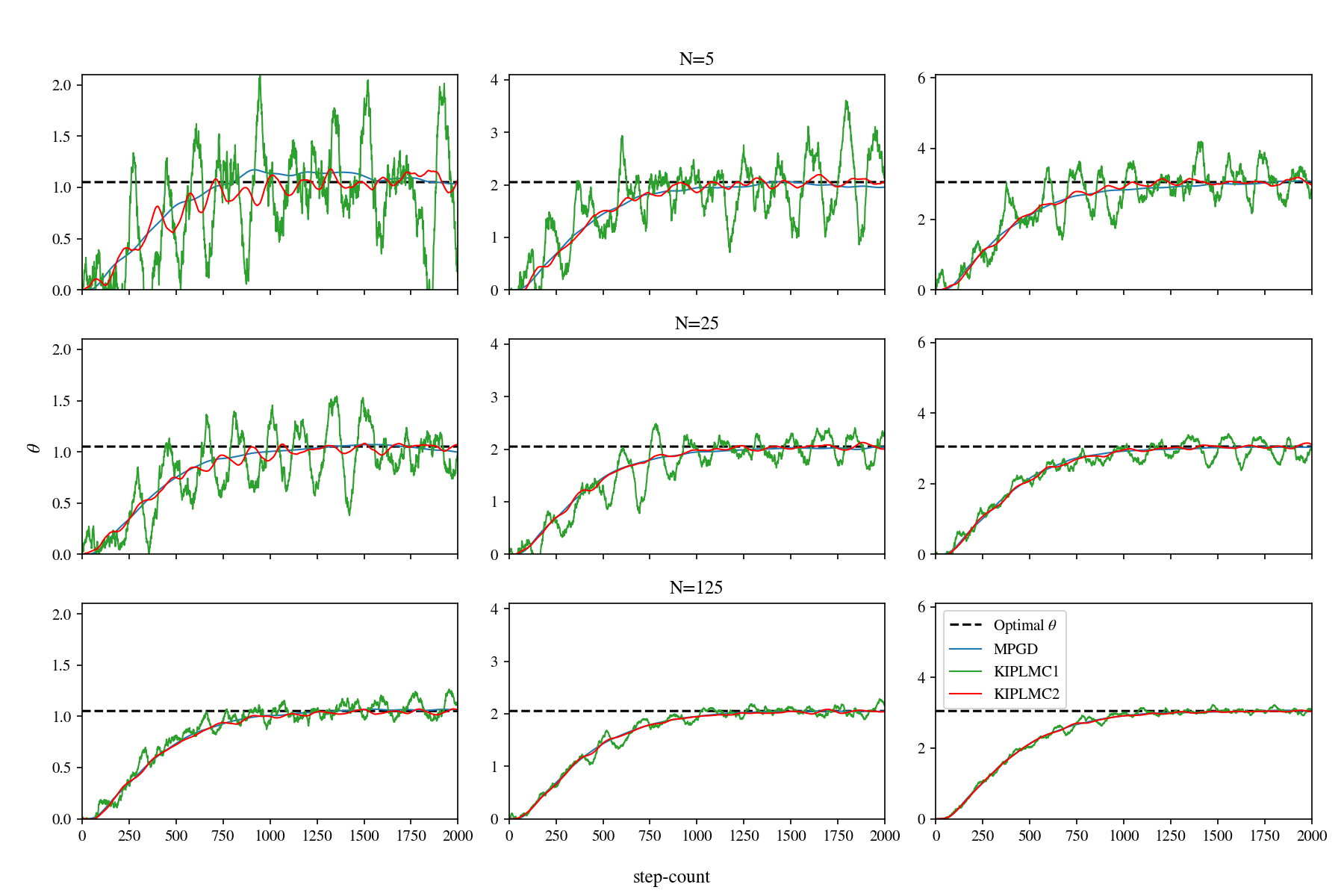
Figure 1: We compare the performance of the MPGD, KIPLMC1, and KIPLMC2 algorithms on the synthetic dataset with true $\bar{\theta}_{\star}\in[1,2,3]$. We observe the desired convergence of behaviours for larger values of $N$. For all the algorithms, with the chosen $\gamma$, we observe momentum effects, which extend to the noise, as can be seen in the oscillations in the low particle number regimes. In this example $d_{x}=d_{\theta}=3$, $d_{y}=500$ and $\gamma=1.2$. $Z_{0}$ is set as $\delta$, the point measure on the origin.

Remark 1 (On H1 and H2).

We will discuss this problem and our assumptions. From (12) it is quite straightforward to observe that,

$$\|\nabla U(z)-\nabla U(z^{\prime})\|\leq \frac{2}{\sigma^{2}}(\|x-x^{\prime}\|+\|\theta-\theta^{\prime}\|)+\sum_{j=1}^{d_{y}}|s(v_{j}^{\intercal}x)-s(v_{j}^{\intercal}x^{\prime})|\|v_{j}\|$$

$$\leq (\frac{2}{\sigma^{2}}+\frac{1}{4}\sum_{j=1}^{d_{y}}\|v_{j}\|^{2})\|z-z^{\prime}\|.$$

This follows from the fact that the logistic function is Lipschitz continuous with constant ${1}/{4}$ [2]. Hence, H2 is satisfied.

For H1, consider

$$\nabla^{2}U(z)=\frac{1}{\sigma^{2}}\begin{pmatrix}I_{d_{\theta}}&-I_{d_{x}}\\ -I_{d_{x}}&I_{d_{\theta}}\end{pmatrix}+\sum_{j=1}^{d_{y}}s(v_{j}^{\intercal}x)(1-s(v_{j}^{\intercal}x))v_{j}\otimes v_{j}.$$

The sum is positive definite and the matrix was shown by [45] to have $2d_{\theta}$ positive eigenvalues and so it follows that $\nabla^{2}U$ is positive definite. Hence $U$ is strictly convex and in theory no lower bound for strong convexity constant exists. We show however this is not a problem for our practical implementations.

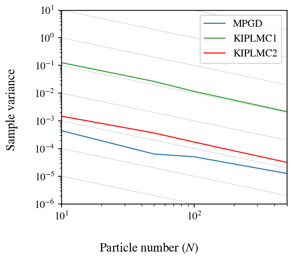
Figure 2: Comparison over 20 Monte Carlo simulations of the algorithms. We compute the sample variance of the algorithms, using the last 500 steps of each simulation. The scales are logarithmic and gridlines corresponding to $\frac{1}{N}$ are provided to highlight the rate of convergence.

In Fig. 1 we can see the difference in the behaviours between the algorithms. Most notably, the KIPLMC2 algorithm exhibits comparable levels of variance as the MPGD algorithm in the $\theta$-dimension, whilst the KIPLMC1 algorithm has much greater variance (roughly 100 times greater). It is interesting to note that the KIPLMC2 algorithm preserves many theoretical properties of the KIPLMC1 algorithm, with empirical variance reduction properties. As $N$ grows the $\theta$ iterates concentrate onto the MMLE $\bar{\theta}_{\star}$ for all algorithms. This behaviour can be seen in more detail in Fig. 2, in which we can observe the variance changing with rate $\mathcal{O}(1/N)$.

Note that the momentum effects of the KIPLMC1 and KIPLMC2 algorithms has been dampened through a specific choice of $\gamma$. In training it was observed that the convergence rate is very sensitive to the choice of $\gamma$, where choices too small exhibit large momentum effects and too large lead to slow convergence. The choice of $\gamma$ here is far from optimal, but allows us to observe the strength of the proposed algorithms.

5.2 Wisconsin Cancer Data

We follow again an experimental prodecure that is similar to the one outlinedin [45] and [2] and make comparisons between the algorithms on a more realistic dataset: the Wisconsin Cancer Data. Again, we use the logistic regression LVM model, outlined above. This task is a binary classification, to determine from 9 “features” gathered from tumors and 693 data points labelled as either benign or malignant. The latent variables correspond to the “features” extracted from the data. The task in this case is to seek to model the behaviour as accurately as possible through the logistic regression LVM.

For this setup we define our probability model as,

$$p_{\theta}(x)=\mathcal{N}(x;\theta\mathbbm{1}_{d_{x}},5I_{d_{x}})$$

and the likelihood as,

$$p(y|x)=\prod_{j=1}^{d_{y}}s(v_{j}^{\intercal}x)^{y_{j}}(1-s(v_{j}^{\intercal}x))^{1-y_{j}}.$$

Note that the parameter $\theta$ is a scalar in this case, hence, this turns out to be a simplified version of the setup described above and so the discussion in Remark 1 is still valid. As opposed to the previous case with synthetic data, here we consider a real dataset, thus we do not have access to the true dataset. Hence, there is no comparison to a $\bar{\theta}_{\star}$, but we can see that different algorithms attain similar values as the estimate of this minimum.

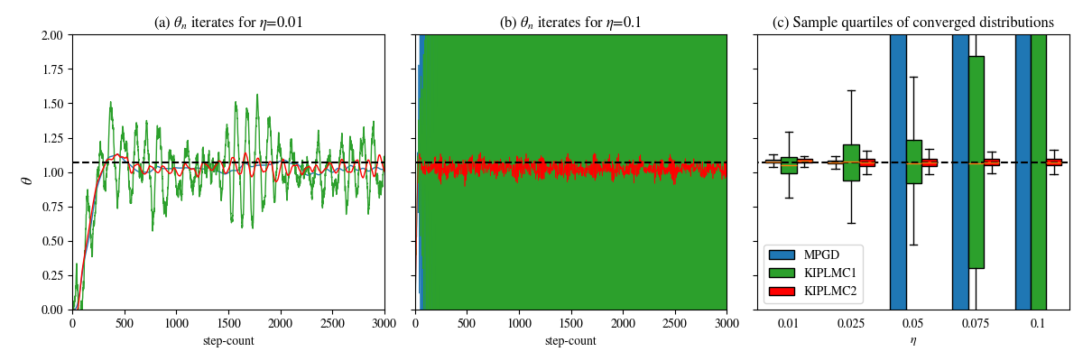
Figure 3: The performance of MPGD, KIPLMC1 and KIPLMC2 algorithms are compared on a logistic regression experiment for the Wisconsin Cancer Dataset. In (a), we show the behaviour of the $\theta_{n}$ iterates for the small step-size of $\eta=0.01$, where all algorithms converge as desired. (b) shows the behaviour $\theta_{n}$ iterates for a step-size where all algorithms except for KIPLMC2 explode. In (c) we compare the distributions of the algorithms over different step-sizes. Observe, that as the step-size $\eta$ increases, the variance of all algorithms increases and MPGD fails at $\eta=0.05$. The particle number, is chosen to be $N=50$ and $\gamma=1.2$.

Most notably in this experiment, we can observe in Fig. 3 the importance of the discretisation KIPLMC2. In particular, this algorithm displays great stability w.r.t. the choice of the step-size. For small values of the step-size, the MPGD algorithm performs with the lowest variance in all cases where it converges, until it explodes where step-sizes become too large. Again, we note that the KIPLMC1 algorithm exhibits more variance in the $\theta$ estimation than the KIPLMC2 algorithm, which has more variance than the MPGD. This is typically an advantage when working with convex problems, but this “sticky” behaviour might prove detrimental in the non-convex case [36, 2]. The injection of noise into the parameter estimation may help the method to escape local minima [4].

In these algorithms one can observe the strength of the KIPLMC2 algorithm, with fast convergence and smoother paths. The latter observation may be related to the differing orders of the algorithms in [51] and [23].

6 Conclusions

This paper extends a line of work on interacting particle, and more generally diffusion-based, algorithms for maximum marginal likelihood estimation. This paper has focused on considering alternatives to the IPSs proposed by [45, 2, 47] for the MMLE problem by considering an accelerated variant. We have shown that we can leverage the existing literature on underdamped Langevin diffusion for sampling [23, 18, 51, 49] to produce two algorithms with greater stability, added smoothness and exponential convergence, which concentrate onto the MMLE with known bounds on the estimation error ${\mathbb{E}}\|\theta_{n}-\bar{\theta}_{\star}\|^{2}$. These algorithms are both based on a momentum-based diffusion - which can both be seen as a relaxation of the friction of the IPLA in [2] or as a noised version of the MPGD in [47]. Empirically, the algorithms perform well compared to the MPGD (with equal choice of step-sizes and friction coefficients) and the diffusions come equipped with stronger theoretical guarantees for sampling. Specifically, the induced noise should improve guarantees in the non-convex setting, as discussed in [2, 55], at a small cost when we consider the variance difference between the MPGD algorithm and KIPLMC2.

The results presented here, hold under very strict assumptions of gradient-Lipschitzness and strong log-concavity, however, following the work done in [69] and [42], it should be possible to extend these results to the non-convex and non-Lipschitz cases. Another interesting direction is to consider the setting in [34]. Similar ideas can be considered within the setting of Stein variational gradient descent as done in [61].

Appendix A Preliminary results

Lemma A.1 (KIPLD as an underdamped Langevin Diffusion).

The KIPLD diffusion can be equivalently written as a single $d_{\theta}+Nd_{x}$-dimensional underdamped Langevin diffusion given by

$${\mathrm{d}}{\mathbf{Z}}_{t} =\bar{{\mathbf{V}}}_{t}^{z}{\mathrm{d}}t,$$ (13)

$${\mathrm{d}}\bar{{\mathbf{V}}}_{t}^{z} =-{\gamma}\bar{{\mathbf{V}}}_{t}^{z}{\mathrm{d}}t-\nabla_{z}\bar{U}_{N}({\mathbf{Z}}_{t}){\mathrm{d}}t+\sqrt{\frac{2{\gamma}}{N}}{\mathrm{d}}{\mathbf{B}}_{t},$$

where ${\mathbf{Z}}_{t}^{i}=N^{-1/2}{\mathbf{X}}_{t}^{i}$ for $i=1,\ldots,N$, ${\mathbf{Z}}_{t}=(\bm{\theta}_{t},{\mathbf{Z}}_{t}^{1},\ldots,{\mathbf{Z}}_{t}^{N})^{\top}\in{\mathbb{R}}^{d_{\theta}+Nd_{x}}$, $\bar{{\mathbf{V}}}_{t}^{z_{i}}=N^{-1/2}{\mathbf{V}}_{t}^{x_{i}}$ and $\bar{{\mathbf{V}}}_{t}^{z}=({\mathbf{V}}_{t}^{\theta},\bar{{\mathbf{V}}}_{t}^{z_{1}},\ldots,\bar{{\mathbf{V}}}_{t}^{z_{N}})^{\top}\in{\mathbb{R}}^{d_{\theta}+Nd_{x}}$, $({\mathbf{B}}_{t})_{t\geq 0}$ is a ${\mathbb{R}}^{d_{\theta}+Nd_{x}}$-valued Brownian motion, and

$$\bar{U}_{N}(\theta,z_{1},\ldots,z_{N}):=\frac{1}{N}\sum_{i=1}^{N}U(\theta,\sqrt{N}z_{i}).$$

Proof.

Recall the KIPLD system:

$$\mathrm{d}\bm{\theta}_{t} ={\mathbf{V}}^{\theta}_{t}\mathrm{d}t$$

$$\mathrm{d}{\mathbf{X}}^{i}_{t} ={\mathbf{V}}^{x_{i}}_{t}\mathrm{d}t,\qquad\text{for }i=1,\ldots,N$$

$$\mathrm{d}{\mathbf{V}}^{\theta}_{t} =-\gamma{\mathbf{V}}^{\theta}_{t}\mathrm{d}t-\frac{1}{N}\sum_{i=1}^{N}\nabla_{\theta}U(\bm{\theta}_{t},{\mathbf{X}}^{i}_{t})\mathrm{d}t+\sqrt{\frac{2\gamma}{N}}\mathrm{d}{\mathbf{B}}^{0}_{t}$$

$$\mathrm{d}{\mathbf{V}}^{x_{i}}_{t} =-\gamma{\mathbf{V}}_{t}^{x_{i}}\mathrm{d}t-\nabla_{x}U(\bm{\theta}_{t},{\mathbf{X}}_{t}^{i})\mathrm{d}t+\sqrt{2\gamma}\mathrm{d}{\mathbf{B}}_{t}^{i},\qquad\text{for }i\in[N]$$

We note now that, below, we generically use the gradient functions $\nabla_{\theta}U(\theta,x):\mathbb{R}^{d_{\theta}}\times\mathbb{R}^{d_{x}}\to\mathbb{R}^{d_{\theta}}$ and $\nabla_{x}U(\theta,x):\mathbb{R}^{d_{\theta}}\times\mathbb{R}^{d_{x}}\to\mathbb{R}^{d_{x}}$ even though their arguments may change. In other words, below $\nabla_{\theta}U(\theta,x)$ denotes the gradient of $U$ with respect to its first argument and $\nabla_{x}U(\theta,x)$ denotes the gradient of $U$ with respect to its second argument.

Let us introduce the following function:

$$U_{N}(\theta,x)=U(\theta,\sqrt{N}x),$$

where we note that the (full) gradient is given as,

$$\nabla U_{N}(\theta,x)=\begin{pmatrix}\nabla_{\theta}U(\theta,\sqrt{N}x)\\ N^{-1/2}\nabla_{x}U(\theta,\sqrt{N}x)\end{pmatrix}.$$

Let us now introduce $z_{\theta}\in\mathbb{R}^{d_{\theta}}$ and $z_{x}=(z_{1},\dots,z_{N})^{T}$ where $z_{i}\in\mathbb{R}^{d_{x}}$ for $i=1,\ldots,N$. We define

$$\bar{U}_{N}(z_{\theta},z_{x})=\frac{1}{N}\sum_{i=1}^{N}U_{N}(z_{\theta},z_{i}).$$ (14)

The gradients are given as

$$\nabla_{z_{\theta}}\bar{U}_{N}(z_{\theta},z_{x})=\frac{1}{N}\sum_{i=1}^{N}\nabla_{\theta}U(z_{\theta},\sqrt{N}z_{x}^{i}),\qquad\nabla_{z_{x}}\bar{U}_{N}(z_{\theta},z_{x})=\begin{pmatrix}N^{-1/2}\nabla_{x}U(z_{\theta},\sqrt{N}z_{1})\\ \vdots\\ N^{-1/2}\nabla_{x}U(z_{\theta},\sqrt{N}z_{N})\end{pmatrix}.$$ (15)

Next, let ${\mathbf{Z}}_{t}^{i}=N^{-1/2}{\mathbf{X}}_{t}^{i}$ for $i=1,\ldots,N$, ${\mathbf{Z}}_{t}=(\bm{\theta}_{t},{\mathbf{Z}}_{t}^{1},\ldots,{\mathbf{Z}}_{t}^{N})^{\top}\in{\mathbb{R}}^{d_{\theta}+Nd_{x}}$, $\bar{{\mathbf{V}}}_{t}^{z_{i}}=N^{-1/2}{\mathbf{V}}_{t}^{x_{i}}$ and $\bar{{\mathbf{V}}}_{t}^{z}=({\mathbf{V}}_{t}^{\theta},\bar{{\mathbf{V}}}_{t}^{z_{1}},\ldots,\bar{{\mathbf{V}}}_{t}^{z_{N}})^{\top}\in{\mathbb{R}}^{d_{\theta}+Nd_{x}}$. We can rewrite the system KIPLD as

$${\mathrm{d}}{\mathbf{Z}}_{t} =\bar{{\mathbf{V}}}_{t}^{z}{\mathrm{d}}t,$$ (16)

$${\mathrm{d}}{{\mathbf{V}}}^{\theta}_{t} =-\gamma{{\mathbf{V}}}^{\theta}_{t}{\mathrm{d}}t-\frac{1}{N}\sum_{i=1}^{N}\nabla_{\theta}U(\bm{\theta}_{t},\sqrt{N}{\mathbf{Z}}_{t}^{i}){\mathrm{d}}t+\sqrt{\frac{2\gamma}{N}}{\mathrm{d}}{\mathbf{B}}_{t}^{0},$$

$${\mathrm{d}}\bar{{\mathbf{V}}}_{t}^{z_{i}} =-\gamma\bar{{\mathbf{V}}}_{t}^{z_{i}}{\mathrm{d}}t-N^{-1/2}\nabla_{x}U(\bm{\theta}_{t},\sqrt{N}{\mathbf{Z}}_{t}^{i}){\mathrm{d}}t+\sqrt{\frac{2\gamma}{N}}{\mathrm{d}}{\mathbf{B}}_{t}^{i},\qquad\text{for }i\in[N].$$

where ${\mathbf{B}}^{0}_{t}$ is a ${\mathbb{R}}^{d_{\theta}}$-valued Brownian motion and ${\mathbf{B}}^{i}_{t}$ for $i=1,\ldots,N$ are ${\mathbb{R}}^{d_{x}}$-valued Brownian motions. Rewriting the system (16) in terms of $\bar{U}_{N}$, using (15), we obtain the result. $\Box$

We can also write the KIPLD in the following alternative way which will ease the analysis.

Lemma A.2 (KIPLD as a standard underdamped Langevin Diffusion).

The KIPLD diffusion can also be written as a single $d_{\theta}+Nd_{x}$-dimensional underdamped Langevin diffusion given by

$${\mathrm{d}}\widetilde{{\mathbf{Z}}}_{t} =\widetilde{{\mathbf{V}}}_{t}^{z}{\mathrm{d}}t,$$ (17)

$${\mathrm{d}}\widetilde{{\mathbf{V}}}_{t}^{z} =-\widetilde{\gamma}\widetilde{{\mathbf{V}}}_{t}^{z}{\mathrm{d}}t-N\nabla_{z}\bar{U}_{N}(\widetilde{{\mathbf{Z}}}_{t}){\mathrm{d}}t+\sqrt{{2{\widetilde{\gamma}}}}{\mathrm{d}}{\mathbf{B}}_{t},$$

where $\widetilde{{\mathbf{Z}}}_{t},\widetilde{{\mathbf{V}}}_{t}^{z}\in\mathbb{R}^{d_{x}+Nd_{\theta}}$ are given as,

$$\widetilde{{\mathbf{Z}}}_{t}=(\bm{\theta}_{\sqrt{N}t},N^{-1/2}{\mathbf{X}}^{1}_{\sqrt{N}t},\dots N^{-1/2}{\mathbf{X}}^{N}_{\sqrt{N}t})^{\intercal},\qquad\widetilde{{\mathbf{V}}}_{t}^{z}=(\sqrt{N}{\mathbf{V}}^{\theta}_{\sqrt{N}t},{\mathbf{V}}^{x_{1}}_{\sqrt{N}t},\dots,{\mathbf{V}}^{x_{N}}_{\sqrt{N}t})^{\intercal},$$

$({\mathbf{B}}_{t})_{t\geq 0}$ is a ${\mathbb{R}}^{d_{\theta}+Nd_{x}}$-valued Brownian motion, $\tilde{\gamma}=\sqrt{N}\gamma$ and

$$\bar{U}_{N}(\theta,z_{1},\ldots,z_{N}):=\frac{1}{N}\sum_{i=1}^{N}U(\theta,z_{i}).$$

Proof.

We use [23, Lemma 1] to prove this result. Consider the variables $\widetilde{{\mathbf{Z}}}_{t}$ and $\widetilde{{\mathbf{V}}}_{t}^{z}$. It is straightforward to observe that

$${\mathrm{d}}\widetilde{{\mathbf{Z}}}_{t}=\widetilde{{\mathbf{V}}}_{t}^{z}{\mathrm{d}}t.$$

Indeed the space rescaling accounts for the time-rescaling in the dynamics of $\widetilde{{\mathbf{Z}}}_{t}$. Now observe that

$${\mathrm{d}}\widetilde{{\mathbf{V}}}^{\theta}_{t} =-N\gamma{\mathbf{V}}^{\theta}_{\sqrt{N}t}{\mathrm{d}}t-\nabla_{\theta}\sum_{i=1}^{N}U(\bm{\theta}_{\sqrt{N}t},{\mathbf{X}}^{i}_{\sqrt{N}t}){\mathrm{d}}t+\sqrt{2\gamma\sqrt{N}}{\mathrm{d}}{\mathbf{B}}_{t}^{0}$$

$$=-\sqrt{N}\gamma\widetilde{{\mathbf{V}}}_{t}^{\theta}{\mathrm{d}}t-N\nabla_{\theta}\bar{U}_{N}(\widetilde{{\mathbf{Z}}}_{t}){\mathrm{d}}t+\sqrt{2\gamma\sqrt{N}}{\mathrm{d}}{\mathbf{B}}_{t}^{0}.$$

Similarly we obtain for $i\in[N]$,

$${\mathrm{d}}\widetilde{{\mathbf{V}}}_{t}^{x_{i}} =-\sqrt{N}\gamma{\mathbf{V}}^{i}_{\sqrt{N}t}{\mathrm{d}}t-\nabla_{x}U(\bm{\theta}_{\sqrt{N}t},{\mathbf{X}}^{i}_{\sqrt{N}t}){\mathrm{d}}t+\sqrt{2\gamma\sqrt{N}}{\mathrm{d}}B_{t}^{i}$$

$$=-\sqrt{N}\gamma\widetilde{{\mathbf{V}}}_{t}^{x_{i}}{\mathrm{d}}t-\nabla_{x}\bar{U}_{N}(\widetilde{{\mathbf{Z}}}_{t}){\mathrm{d}}t+\sqrt{2\gamma\sqrt{N}}{\mathrm{d}}B_{t}^{i},$$

where we recall our definition of the gradient of $\bar{U}_{N}$ from (15) to obtain the correct scaling in front of $\nabla_{x}\bar{U}_{N}(\widetilde{{\mathbf{Z}}}_{t})$. Now, taking $\tilde{\gamma}=\sqrt{N}\gamma$, the result follows. $\Box$

Recall that the algorithms proposed seek to target with the $n$th step the analytic solution at time $n\eta$, where $\eta$ is the step-size of the algorithm for the rescaled system. Hence, by re-scaling $\bar{\eta}=\frac{\eta}{\sqrt{N}}$, we can use algorithms for the rescaled system to produce estimates for KIPLMC1 and KIPLMC2. This is discussed below in B.4 and B.5. Given these results, it is natural to explore the properties of the function $\bar{U}_{N}$, as this new potential plays a crucial role in both rescalings. We note below some properties of $\bar{U}_{N}$ which will be useful in the proofs.

Lemma A.3 (Stationary measure for (17)).

The measure $\tilde{\pi}$, left stationary by the dynamics of (17), is given as

$$\tilde{\pi}({\mathrm{d}}\tilde{z},{\mathrm{d}}\tilde{v})\propto\exp\left(-N\bar{U}_{N}(\tilde{z})-\frac{1}{2}\|\tilde{v}\|^{2}\right){\mathrm{d}}\tilde{z}{\mathrm{d}}\tilde{v},$$ (18)

for all $\tilde{z},\tilde{v}\in\mathbb{R}^{d_{z}}$.

This result follows directly by observing the rescaling given in Lemma A.2, both in the parameters and equation. For a discussion of the stationary measure of a standard underdamped Langevin diffusion see [53, Chapter 6].

Lemma A.4 (Strong convexity of $\bar{U}_{N}$).

Under H1, the function $\bar{U}_{N}:{\mathbb{R}}^{d_{\theta}+Nd_{x}}\to{\mathbb{R}}$ as defined in (14) is $\mu$-strongly convex

$$\langle z-z^{\prime},\nabla\bar{U}_{N}(z)-\nabla\bar{U}_{N}(z^{\prime})\rangle\geq\mu\|z-z^{\prime}\|^{2},$$

for all $z,z^{\prime}\in{\mathbb{R}}^{d_{\theta}+Nd_{x}}$ and $N\in{\mathbb{N}}$.

Proof.

Let $z=(z_{\theta},z_{1},\ldots,z_{N})$ and $z^{\prime}=(z_{\theta}^{\prime},z_{1}^{\prime},\ldots,z_{N}^{\prime})$. We have

$$\langle z-z^{\prime},\nabla\bar{U}_{N}(z)-\nabla\bar{U}_{N}(z^{\prime})\rangle =\left\langle\begin{pmatrix}z_{\theta}-z_{\theta}^{\prime}\\ z_{1}-z_{1}^{\prime}\\ \vdots\\ z_{N}-z_{N}^{\prime}\end{pmatrix},\begin{pmatrix}(1/N)\sum_{i=1}^{N}\nabla_{\theta}\left(U(z_{\theta},\sqrt{N}z_{i})-\nabla_{\theta}U(z_{\theta}^{\prime},\sqrt{N}z_{i}^{\prime})\right)\\ N^{-1/2}\nabla_{x}U(z_{\theta},\sqrt{N}z_{1})-N^{-1/2}\nabla_{x}U(z_{\theta}^{\prime},\sqrt{N}z_{1}^{\prime})\\ \vdots\\ N^{-1/2}\nabla_{x}U(z_{\theta},\sqrt{N}z_{N})-N^{-1/2}\nabla_{x}U(z_{\theta}^{\prime},\sqrt{N}z_{N}^{\prime})\end{pmatrix}\right\rangle$$

$$=\frac{1}{N}\sum_{i=1}^{N}\left(\langle z_{\theta}-z_{\theta}^{\prime},\nabla_{\theta}U(z_{\theta},\sqrt{N}z_{i})-\nabla_{\theta}U(z_{\theta}^{\prime},\sqrt{N}z_{i}^{\prime})\rangle\right)$$

$$\quad+\frac{1}{N}\sum_{i=1}^{N}\langle N^{1/2}z_{i}-N^{1/2}z_{i}^{\prime},\nabla_{x}U(z_{\theta},\sqrt{N}z_{i})-\nabla_{x}U(z_{\theta}^{\prime},\sqrt{N}z_{i}^{\prime})\rangle.$$

Next, H1 implies that

$$\langle z-z^{\prime},\nabla\bar{U}_{N}(z)-\nabla\bar{U}_{N}(z^{\prime})\rangle\geq\frac{1}{N}\sum_{i=1}^{N}\mu\left(\|z_{\theta}-z_{\theta}^{\prime}\|^{2}+N\|z_{i}-z_{i}^{\prime}\|^{2}\right)=\mu\|z-z^{\prime}\|^{2}.$$

This completes the proof. $\Box$

Next, we show that the function $\bar{U}_{N}$ is $L$-gradient Lipschitz.

Lemma A.5 (Gradient Lipschitzness of $\bar{U}_{N}$).

Under H2, the function $\bar{U}_{N}:{\mathbb{R}}^{d_{\theta}+Nd_{x}}\to{\mathbb{R}}$ as defined in (14) is $L$-gradient Lipschitz

$$\|\nabla\bar{U}_{N}(z)-\nabla\bar{U}_{N}(z^{\prime})\|\leq L\|z-z^{\prime}\|,$$

for all $z,z^{\prime}\in{\mathbb{R}}^{d_{\theta}+Nd_{x}}$ and $N\in{\mathbb{N}}$.

Proof.

Let $z=(z_{\theta},z_{1},\ldots,z_{N})$ and $z^{\prime}=(z_{\theta}^{\prime},z_{1}^{\prime},\ldots,z_{N}^{\prime})$. Then

$$\|\nabla\bar{U}_{N}(z)-\nabla\bar{U}_{N}(z^{\prime})\|^{2} =\left\|\begin{pmatrix}(1/N)\sum_{i=1}^{N}\nabla_{\theta}U(z_{\theta},\sqrt{N}z_{i})-\nabla_{\theta}U(z_{\theta}^{\prime},\sqrt{N}z_{i}^{\prime})\\ N^{-1/2}\nabla_{x}U(z_{\theta},\sqrt{N}z_{1})-N^{-1/2}\nabla_{x}U(z_{\theta}^{\prime},\sqrt{N}z_{1}^{\prime})\\ \vdots\\ N^{-1/2}\nabla_{x}U(z_{\theta},\sqrt{N}z_{N})-N^{-1/2}\nabla_{x}U(z_{\theta}^{\prime},\sqrt{N}z_{N}^{\prime})\end{pmatrix}\right\|^{2}$$

$$=\left\|\frac{1}{N}\sum_{i=1}^{N}\left(\nabla_{\theta}U(z_{\theta},\sqrt{N}z_{i})-\nabla_{\theta}U(z_{\theta}^{\prime},\sqrt{N}z_{i}^{\prime})\right)\right\|^{2}$$

$$\quad+\frac{1}{N}\sum_{i=1}^{N}\left\|\nabla_{x}U(z_{\theta},\sqrt{N}z_{i})-\nabla_{x}U(z_{\theta}^{\prime},\sqrt{N}z_{i}^{\prime})\right\|^{2}.$$

Using the fact that $(\cdot)^{2}$ is a convex function and Jensen’s inequality for the first term, we obtain

$$\|\nabla\bar{U}_{N}(z)-\nabla\bar{U}_{N}(z^{\prime})\|^{2} \leq\frac{1}{N}\sum_{i=1}^{N}\left\|\nabla_{\theta}U(z_{\theta},\sqrt{N}z_{i})-\nabla_{\theta}U(z_{\theta}^{\prime},\sqrt{N}z_{i}^{\prime})\right\|^{2}$$

$$\quad+\frac{1}{N}\sum_{i=1}^{N}\left\|\nabla_{x}U(z_{\theta},\sqrt{N}z_{i})-\nabla_{x}U(z_{\theta}^{\prime},\sqrt{N}z_{i}^{\prime})\right\|^{2}.$$

Using H2, we have

$$\|\nabla\bar{U}_{N}(z)-\nabla\bar{U}_{N}(z^{\prime})\|^{2} \leq\frac{L^{2}}{N}\sum_{i=1}^{N}\left(\|z_{\theta}-z_{\theta}^{\prime}\|^{2}+N\|z_{i}-z_{i}^{\prime}\|^{2}\right)$$

$$=L^{2}\|z-z^{\prime}\|^{2},$$

which completes the proof. $\Box$

Appendix B Proofs

B.1 Proof of Proposition 1

Given Lemma A.1, the system (13) has a positive recurrent Markov stationary measure, absolutely continuous with respect to the Lebesgue measure, given by the density [32]

$$\bar{\pi}^{N}(z,\bar{v})\propto\exp\left(-N\bar{U}_{N}(z)-\frac{N}{2}\|\bar{v}\|^{2}\right),$$

where $\bar{U}_{N}$ is given in (14). Note, this follows from eqs. (1.1) and (1.3) in [32] by putting $U:=N\bar{U}_{N}$ and $u=N^{-1}$. Let $z=(\theta,z_{1},\ldots,z_{N})$. Using (14), we have

$$\bar{\pi}(z,\bar{v}) \propto\exp\left(-\sum_{i=1}^{N}U(\theta,\sqrt{N}z_{i})-\frac{N}{2}\|\bar{v}\|^{2}\right).$$

Let us now look at $\theta$-marginal of this density, which can be written as

$$\pi^{N}_{\Theta}(\theta)\propto\int_{\mathbb{R}^{Nd_{x}+d_{\theta}}}\int_{\mathbb{R}^{Nd_{x}}}e^{-\sum_{i=1}^{N}U(\theta,\sqrt{N}z_{i})-\frac{N}{2}\|\bar{v}^{z}\|^{2}}{\mathrm{d}}z_{x}{\mathrm{d}}\bar{v}.$$

where $z_{x}=(z_{1},\ldots,z_{N})\in{\mathbb{R}}^{Nd_{x}}$. Note now that, integrating out $\bar{v}$, using a change of variables $x_{i}^{\prime}=\sqrt{N}z_{i}$, and setting $x^{\prime}=(x_{1}^{\prime},\ldots,x_{N}^{\prime})$, we have

$$\pi^{N}_{\Theta}(\theta) \propto{N}^{-1/2}\int_{\mathbb{R}^{Nd_{x}}}e^{-\sum_{i=1}^{N}U(\theta,x^{\prime}_{i})}{\mathrm{d}}x^{\prime},$$

$$\propto\left(\int_{{\mathbb{R}}^{d_{x}}}e^{-U(\theta,x^{\prime})}{\mathrm{d}}x^{\prime}\right)^{N}=\exp(N\log p_{\theta}(y)),$$

since $p_{\theta}(y)=\int e^{-U(\theta,x)}{\mathrm{d}}x$ by definition where $U(\theta,x)=-\log p_{\theta}(x,y)$.

B.2 Proof of Proposition 2

Note that, by H1, $U(\theta,x)$ is jointly $\mu$-strongly convex. Let $\kappa(\theta)=-\log p_{\theta}(y)$. Using the Prekopa-Leindler inequality for strongly log-concave distributions [60, Theorem 3.8], we can see that

$$\langle\theta-\theta^{\prime},\nabla\kappa(\theta)-\nabla\kappa(\theta)\rangle\geq\mu\|\theta-\theta^{\prime}\|^{2}.$$

The bound then follows using an identical proof of Proposition 3 in [2].

B.3 Proof of Proposition 3

The proof follows from Lemma A.1 which shows that we can rewrite the KIPLD system as a single $d_{\theta}+Nd_{x}$-dimensional underdamped Langevin diffusion. Then with a suitable time rescaling (see Lemma 1 in [23]), we can rewrite this diffusion as a standard underdamped diffusion as shown in Lemma A.2. The result then follows from the exponential convergence of the underdamped Langevin diffusion [23, Theorem 1] with suitable modifications, e.g., see the proof of [42, Theorem 8.7]. The result then follows from the fact that $W_{2}$ between marginals are bounded by the $W_{2}$ between joint distributions.

B.4 Proof of Theorem 1

By Lemma A.2, we have the standard underdamped diffusion

$${\mathrm{d}}\widetilde{{\mathbf{Z}}}_{t} =\widetilde{{\mathbf{V}}}_{t}^{z}{\mathrm{d}}t,$$ (19)

$${\mathrm{d}}\widetilde{{\mathbf{V}}}_{t}^{z} =-\widetilde{\gamma}\widetilde{{\mathbf{V}}}_{t}^{z}{\mathrm{d}}t-N\nabla_{z}\bar{U}_{N}(\widetilde{{\mathbf{Z}}}_{t}){\mathrm{d}}t+\sqrt{{2{\widetilde{\gamma}}}}{\mathrm{d}}{\mathbf{B}}_{t}.$$

It is apparent that the stationary measure of this scheme is

$$\widetilde{\pi}(z,v)\propto e^{-N\bar{U}_{N}(z)-\frac{1}{2}\|v\|^{2}}.$$

We will now look at the standard kinetic Langevin Monte Carlo discretisation of the SDE in (19) and show that this scheme coincides with KIPLMC1. Thus we can utilize the bounds in [23] directly for our scheme.

Let us write the Exponential Integrator discretisation of this scheme (abusing the notation using same letters) using the step-size $\tilde{\eta}$

$$\widetilde{{\mathbf{Z}}}_{n+1} =\widetilde{{\mathbf{Z}}}_{n}+\widetilde{\psi}_{1}(\tilde{\eta})\widetilde{{\mathbf{V}}}_{n}^{z}-\widetilde{\psi}_{2}(\tilde{\eta})N\nabla\bar{U}_{N}(\widetilde{{\mathbf{Z}}}_{n})+\sqrt{2\tilde{\gamma}}\tilde{\varepsilon}_{n+1},$$ (20)

$$\widetilde{{\mathbf{V}}}_{n+1}^{z} =\widetilde{\psi}_{0}(\tilde{\eta})\widetilde{{\mathbf{V}}}_{n}^{z}-\widetilde{\psi}_{1}(\tilde{\eta})N\nabla\bar{U}_{N}(\widetilde{{\mathbf{Z}}}_{n})+\sqrt{2\tilde{\gamma}}\tilde{\varepsilon}_{n+1}^{\prime}.$$

Since the function $z\mapsto N\bar{U}_{N}(z)$ is $N\mu$ strongly convex and $NL$-gradient-Lipschitz, for $\tilde{\gamma}\geq\sqrt{N\mu+NL}$ and $\tilde{\eta}\leq m/(4\tilde{\gamma}L)$, [23, Theorem 2] directly implies that

$$W_{2}(\nu_{n},\bar{\pi})\leq\sqrt{2}\left(1-\frac{0.75\mu\tilde{\eta}}{\tilde{\gamma}}\right)^{n}W_{2}(\nu_{0},\bar{\pi})+\frac{L\tilde{\eta}\sqrt{2d_{z}}}{\mu},$$

where $\nu_{n}$ denotes the law of the discretisation (20) at time $n$ and $\tilde{\pi}$ the stationary measure given in Lemma A.3. We relate the discretisation (20) to KIPLMC1. It is straightforward to check that, after proper modifications, the discretisation (20) coincides with the KIPLMC1 with $\tilde{\eta}=\eta/\sqrt{N}$ and $\tilde{\gamma}=\sqrt{N}\gamma$. Therefore, by specializing this bound to $\theta$-dimension and substituting $\tilde{\eta}=\eta/\sqrt{N}$ and $\tilde{\gamma}=\sqrt{N}\gamma$, we obtain the convergence bound for the KIPLMC1. Combining this with the concentration result from Prop. 2, we obtain the result.

B.5 Proof of Theorem 2

Again, recall by Lemma A.2, we consider our rescaled standard underdamped diffusion, given by (19) and seek to recover from this the behaviour of KIPLMC2. Using this rescaled system we directly apply the results from [51] for our scheme.

We now write the splitting scheme for the diffusion in Lemma A.2, using step-size $\tilde{\eta}$,

$$\widetilde{{\mathbf{Z}}}_{n+1} =\widetilde{{\mathbf{Z}}}_{n}+\tilde{\eta}(\tilde{\delta}\widetilde{{\mathbf{V}}}^{z}_{n}+\sqrt{1-\tilde{\delta}^{2}}\varepsilon_{n+1})-\frac{\tilde{\eta}^{2}}{2}N\nabla\bar{U}_{N}(\widetilde{{\mathbf{Z}}}_{n})$$ (21)

$$\widetilde{{\mathbf{V}}}^{z}_{n+1} =\tilde{\delta}^{2}\widetilde{{\mathbf{V}}}_{n}^{z}-\frac{\tilde{\eta}\tilde{\delta}}{2}(N\nabla\bar{U}_{N}(\widetilde{{\mathbf{Z}}}_{n})+N\nabla\bar{U}_{N}(\widetilde{{\mathbf{Z}}}_{n+1}))+\sqrt{1-\tilde{\delta}^{2}}(\tilde{\delta}\varepsilon_{n+1}+\varepsilon_{n+1}^{\prime}),$$

where $\tilde{\delta}=e^{-\tilde{\gamma}\tilde{\eta}/2}$. Using the $N\,L$-gradient-Lipschitzness and $N\,\mu$ strong convexity of the function $z\mapsto N\bar{U}_{N}(z)$, and with the choice of $\tilde{\gamma}\geq 2\sqrt{NL}$ and $\tilde{\eta}\leq\frac{N\mu}{33\tilde{\gamma}^{3}}$, we apply the results of [51, Theorem 1] and [51, Proposition 11] to obtain

$$W_{2}(\nu_{n},\bar{\pi})\leq C\left(\left(1-\frac{\tilde{\eta}\tilde{\mu}}{\tilde{\gamma}}\right)^{\frac{n}{2}}W_{2}(\nu_{0},\bar{\pi})+\tilde{\eta}\sqrt{2d_{z}}\frac{6\tilde{\gamma}\tilde{K}}{\tilde{\mu}}\right),$$

where $\nu_{n}$ is now the law of the discretisation (21) at time $n$ and $\tilde{\pi}$ the stationary measure from Lemma A.3. Further,

$$C=\sqrt{3}(\sqrt{\tilde{L}}\lor\sqrt{\tilde{L}}^{-1}),\qquad K=\tilde{L}\left(1+e^{\tilde{L}\tilde{\eta}^{2}}\left(\frac{\tilde{\eta}}{6}+\frac{\tilde{\eta}^{2}\tilde{L}}{24}\right)\right)\left(1+\frac{\tilde{\eta}\tilde{L}}{2\sqrt{\tilde{\mu}}}\right).$$

Again, we can recover the behaviour of KIPLMC2 when we set $\tilde{\eta}=\eta/\sqrt{N}$ and $\tilde{\gamma}=\sqrt{N}\gamma$. It is quite easy to see that when we set these parameters and consider the $\theta$-marginal, the $n$th step of this rescaled scheme will now correspond to the $n$th step of the KIPLMC2, provided the initial distribution of both is the same. Combining this with the concentration result from Prop. 2, we obtain the desired result.

Appendix C Results

C.1 Variance from (c) Fig. 3 in tabular form

Table 1: We compare the performance of the different algorithms over increasing step-sizes. Observe, despite the better behaviour at lower step-size $\eta$, the MPGD algorithm is the least stable. We compute the sample variance of the algorithms over 20 Monte Carlo simulations, using the last 500 steps of each simulation.

Sample Variance
Algorithms	$\eta$
	0.01	0.025	0.05	0.075	0.1
MPGD	$\bm{2.30\times 10^{-2}}$	$\bm{2.77\times 10^{-2}}$	1.75$\times 10^{9}$	2.34$\times 10^{50}$	7.78$\times 10^{110}$
KIPLMC1	1.91$\times 10^{-1}$	1.30$\times 10^{-1}$	1.90$\times 10^{-1}$	8.52$\times 10^{-1}$	6.06$\times 10^{17}$
KIPLMC2	2.63$\times 10^{-2}$	3.05$\times 10^{-2}$	$\bm{3.37\times 10^{-2}}$	$\bm{3.03\times 10^{-2}}$	$\bm{3.36\times 10^{-2}}$

References

- [1] Ö. Deniz Akyildiz, Dan Crisan, and Joaquín Míguez. Parallel sequential Monte Carlo for stochastic gradient-free nonconvex optimization. Statistics and Computing, 30(6):1645–1663, 2020.
- [2] Ö Deniz Akyildiz, Francesca Romana Crucinio, Mark Girolami, Tim Johnston, and Sotirios Sabanis. Interacting particle langevin algorithm for maximum marginal likelihood estimation. arXiv preprint arXiv:2303.13429, 2023.
- [3] Ö. Deniz Akyildiz, Michela Ottobre, and Iain Souttar. A multiscale perspective on maximum marginal likelihood estimation. arXiv preprint arXiv:2406.04187, 2024.
- [4] Ö. Deniz Akyildiz and Sotirios Sabanis. Nonasymptotic analysis of stochastic gradient hamiltonian monte carlo under local conditions for nonconvex optimization. Journal of Machine Learning Research, 25(113):1–34, 2024.
- [5] Yves F. Atchade, Gersende Fort, and Eric Moulines. On stochastic proximal gradient algorithms. arXiv:1402.2365, 2014.
- [6] Yves F. Atchadé, Gersende Fort, and Eric Moulines. On perturbed proximal gradient algorithms. Journal of Machine Learning Research, 18(10):1–33, 2017.
- [7] José M Bernardo and Adrian FM Smith. Bayesian theory, volume 405. John Wiley & Sons, 2009.
- [8] David M Blei, Andrew Y Ng, and Michael I Jordan. Latent Dirichlet allocation. Journal of Machine Learning Research, 3(Jan):993–1022, 2003.
- [9] James G Booth and James P Hobert. Maximizing generalized linear mixed model likelihoods with an automated Monte Carlo EM algorithm. Journal of the Royal Statistical Society: Series B (Statistical Methodology), 61(1):265–285, 1999.
- [10] Anastasia Borovykh, Nikolas Kantas, Panos Parpas, and Greg Pavliotis. Optimizing interacting Langevin dynamics using spectral gaps. In Proceedings of the 38th International Conference on Machine Learning (ICML 2021), 2021.
- [11] Nicolas Brosse, Alain Durmus, Éric Moulines, and Sotirios Sabanis. The tamed unadjusted Langevin algorithm. Stochastic Processes and their Applications, 129(10):3638–3663, 2019.
- [12] Olivier Cappé, Arnaud Doucet, Marc Lavielle, and Eric Moulines. Simulation-based methods for blind maximum-likelihood filter identification. Signal Processing, 73(1-2):3–25, 1999.
- [13] Rocco Caprio, Juan Kuntz, Samuel Power, and Adam M. Johansen. Error bounds for particle gradient descent, and extensions of the log-sobolev and talagrand inequalities, 2024.
- [14] Gilles Celeux. The SEM algorithm: a probabilistic teacher algorithm derived from the em algorithm for the mixture problem. Computational Statistics Quarterly, 2:73–82, 1985.
- [15] Gilles Celeux and Jean Diebolt. A stochastic approximation type EM algorithm for the mixture problem. Stochastics: An International Journal of Probability and Stochastic Processes, 41(1-2):119–134, 1992.
- [16] KS Chan and Johannes Ledolter. Monte Carlo EM estimation for time series models involving counts. Journal of the American Statistical Association, 90(429):242–252, 1995.
- [17] Xiang Cheng, Niladri S Chatterji, Yasin Abbasi-Yadkori, Peter L Bartlett, and Michael I Jordan. Sharp convergence rates for Langevin dynamics in the nonconvex setting. arXiv preprint arXiv:1805.01648, 2018.
- [18] Xiang Cheng, Niladri S Chatterji, Peter L Bartlett, and Michael I Jordan. Underdamped Langevin MCMC: A non-asymptotic analysis. In Conference On Learning Theory, pages 300–323, 2018.
- [19] Sinho Chewi, Murat A Erdogdu, Mufan Li, Ruoqi Shen, and Shunshi Zhang. Analysis of Langevin Monte Carlo from Poincare to Log-Sobolev. In Conference on Learning Theory, pages 1–2. PMLR, 2022.
- [20] Arnak Dalalyan. Further and stronger analogy between sampling and optimization: Langevin monte carlo and gradient descent. In Conference on Learning Theory, pages 678–689, 2017.
- [21] Arnak S Dalalyan. Theoretical guarantees for approximate sampling from smooth and log-concave densities. Journal of the Royal Statistical Society: Series B (Statistical Methodology), 79(3):651–676, 2017.
- [22] Arnak S Dalalyan and Avetik Karagulyan. User-friendly guarantees for the Langevin Monte Carlo with inaccurate gradient. Stochastic Processes and their Applications, 129(12):5278–5311, 2019.
- [23] Arnak S Dalalyan and Lionel Riou-Durand. On sampling from a log-concave density using kinetic langevin diffusions. Bernoulli, 26(3):1956–1988, 2020.
- [24] Valentin De Bortoli, Alain Durmus, Marcelo Pereyra, and Ana F Vidal. Efficient stochastic optimisation by unadjusted langevin monte carlo. Statistics and Computing, 31(3):1–18, 2021.
- [25] Arthur P Dempster, Nan M Laird, and Donald B Rubin. Maximum likelihood from incomplete data via the em algorithm. Journal of the Royal Statistical Society: Series B (Methodological), 39(1):1–22, 1977.
- [26] J Diebolt and E HS Ip. A stochastic EM algorithm for approximating the maximum likelihood estimate. In W. R. Gilks, S. T. Richardson, and D. J. Spiegelhalter, editors, Markov Chain Monte Carlo in Practice. CRC Publishers, 1996.
- [27] Randal Douc, Eric Moulines, and David Stoffer. Nonlinear time series: Theory, methods and applications with R examples. CRC press, 2014.
- [28] Jin-Chuan Duan, Andras Fulop, and Yu-Wei Hsieh. Maximum likelihood estimation of latent variable models by SMC with marginalization and data cloning. USC-INET Research Paper, (17-27), 2017.
- [29] Alain Durmus, Szymon Majewski, and Błażej Miasojedow. Analysis of Langevin Monte Carlo via convex optimization. Journal of Machine Learning Research, 20(1):2666–2711, 2019.
- [30] Alain Durmus and Eric Moulines. Nonasymptotic convergence analysis for the unadjusted Langevin algorithm. The Annals of Applied Probability, 27(3):1551–1587, 2017.
- [31] Alain Durmus and Eric Moulines. High-dimensional Bayesian inference via the unadjusted Langevin algorithm. Bernoulli, 25(4A):2854–2882, 2019.
- [32] Andreas Eberle, Arnaud Guillin, and Raphael Zimmer. Couplings and quantitative contraction rates for Langevin dynamics. The Annals of Probability, 47(4):1982–2010, 2019.
- [33] Paula Cordero Encinar, Francesca R Crucinio, and O. Deniz Akyildiz. Proximal interacting particle langevin algorithms. arXiv preprint arXiv:2406.14292, 2024.
- [34] Zhou Fan, Leying Guan, Yandi Shen, and Yihong Wu. Gradient flows for empirical bayes in high-dimensional linear models. arXiv preprint arXiv:2312.12708, 2023.
- [35] Carlo Gaetan and Jian-Feng Yao. A multiple-imputation Metropolis version of the EM algorithm. Biometrika, 90(3):643–654, 2003.
- [36] Xuefeng Gao, Mert Gürbüzbalaban, and Lingjiong Zhu. Global convergence of stochastic gradient hamiltonian monte carlo for non-convex stochastic optimization: Non-asymptotic performance bounds and momentum-based acceleration. Oper. Res., 70:2931–2947, 2018.
- [37] Sara Grassi and Lorenzo Pareschi. From particle swarm optimization to consensus based optimization: stochastic modeling and mean-field limit. Mathematical Models and Methods in Applied Sciences, 31(08):1625–1657, 2021.
- [38] Peter D Hoff, Adrian E Raftery, and Mark S Handcock. Latent space approaches to social network analysis. Journal of the american Statistical association, 97(460):1090–1098, 2002.
- [39] Chii-Ruey Hwang. Laplace’s method revisited: weak convergence of probability measures. The Annals of Probability, pages 1177–1182, 1980.
- [40] Eric Jacquier, Michael Johannes, and Nicholas Polson. MCMC maximum likelihood for latent state models. Journal of Econometrics, 137(2):615–640, 2007.
- [41] Adam M Johansen, Arnaud Doucet, and Manuel Davy. Particle methods for maximum likelihood estimation in latent variable models. Statistics and Computing, 18(1):47–57, 2008.
- [42] Tim Johnston, Iosif Lytras, and Sotirios Sabanis. Kinetic langevin mcmc sampling without gradient lipschitz continuity-the strongly convex case. Journal of Complexity, 2024.
- [43] Tim Johnston, Nikolaos Makras, and Sotirios Sabanis. Taming the interacting particle langevin algorithm–the superlinear case. arXiv preprint arXiv:2403.19587, 2024.
- [44] James Kennedy and Russell Eberhart. Particle swarm optimization. In Proceedings of ICNN’95-international conference on neural networks, volume 4, pages 1942–1948. IEEE, 1995.
- [45] Juan Kuntz, Jen Ning Lim, and Adam M Johansen. Particle algorithms for maximum likelihood training of latent variable models. In International Conference on Artificial Intelligence and Statistics, pages 5134–5180. PMLR, 2023.
- [46] Kenneth Lange. A gradient algorithm locally equivalent to the em algorithm. Journal of the Royal Statistical Society: Series B (Methodological), 57(2):425–437, 1995.
- [47] Jen Ning Lim, Juan Kuntz, Samuel Power, and Adam M Johansen. Momentum particle maximum likelihood. In Proceedings of 41st International Conference on Machine Learning (ICML), volume 235, 2024.
- [48] Chuanhai Liu and Donald B Rubin. The ecme algorithm: a simple extension of em and ecm with faster monotone convergence. Biometrika, 81(4):633–648, 1994.
- [49] Yi-An Ma, Niladri S. Chatterji, Xiang Cheng, Nicolas Flammarion, Peter L. Bartlett, and Michael I. Jordan. Is there an analog of Nesterov acceleration for gradient-based MCMC? Bernoulli, 27(3):1942 – 1992, 2021.
- [50] Xiao-Li Meng and Donald B Rubin. Maximum likelihood estimation via the ecm algorithm: A general framework. Biometrika, 80(2):267–278, 1993.
- [51] Pierre Monmarché. High-dimensional mcmc with a standard splitting scheme for the underdamped langevin diffusion. Electronic Journal of Statistics, 15(2):4117–4166, 2021.
- [52] Edward Nelson. Dynamical Theories of Brownian Motion. Princeton University Press, 1967.
- [53] Grigorios A. Pavliotis. Stochastic processes and applications: Diffusion Processes, the Fokker-Planck and langevin equations. Springer, 2014.
- [54] René Pinnau, Claudia Totzeck, Oliver Tse, and Stephan Martin. A consensus-based model for global optimization and its mean-field limit. Mathematical Models and Methods in Applied Sciences, 27(01):183–204, 2017.
- [55] Maxim Raginsky, Alexander Rakhlin, and Matus Telgarsky. Non-convex learning via Stochastic Gradient Langevin Dynamics: a nonasymptotic analysis. In Conference on Learning Theory, pages 1674–1703, 2017.
- [56] Christian P Robert and George Casella. Monte Carlo statistical methods. John Wiley & Sons, 2004.
- [57] Gareth O Roberts and Osnat Stramer. Langevin diffusions and metropolis-hastings algorithms. Methodology and computing in applied probability, 4(4):337–357, 2002.
- [58] Gareth O Roberts, Richard L Tweedie, et al. Exponential convergence of Langevin distributions and their discrete approximations. Bernoulli, 2(4):341–363, 1996.
- [59] Filippo Santambrogio. Optimal transport for applied mathematicians. Birkäuser, NY, 55(58-63):94, 2015.
- [60] Adrien Saumard and Jon A Wellner. Log-concavity and strong log-concavity: a review. Statistics surveys, 8:45, 2014.
- [61] Louis Sharrock, Daniel Dodd, and Christopher Nemeth. Tuning-free maximum likelihood training of latent variable models via coin betting. In International Conference on Artificial Intelligence and Statistics, pages 1810–1818. PMLR, 2024.
- [62] Robert P Sherman, Yu-Yun K Ho, and Siddhartha R Dalal. Conditions for convergence of Monte Carlo EM sequences with an application to product diffusion modeling. The Econometrics Journal, 2(2):248–267, 1999.
- [63] Paris Smaragdis, Bhiksha Raj, and Madhusudana Shashanka. A probabilistic latent variable model for acoustic modeling. Advances in Models for Acoustic Processing Workshop, NIPS, 148:8–1, 2006.
- [64] Arnaud Vadeboncoeur, Ö. Deniz Akyildiz, Ieva Kazlauskaite, Mark Girolami, and Fehmi Cirak. Fully probabilistic deep models for forward and inverse problems in parametric pdes. Journal of Computational Physics, 491:112369, 2023.
- [65] Santosh Vempala and Andre Wibisono. Rapid convergence of the unadjusted Langevin algorithm: Isoperimetry suffices. Advances in Neural Information Processing Systems, 32, 2019.
- [66] Greg CG Wei and Martin A Tanner. A Monte Carlo implementation of the EM algorithm and the poor man’s data augmentation algorithms. Journal of the American Statistical Association, 85(411):699–704, 1990.
- [67] Nick Whiteley, Annie Gray, and Patrick Rubin-Delanchy. Statistical exploration of the manifold hypothesis. arXiv preprint arXiv:2208.11665, 2022.
- [68] Tatiana Xifara, Chris Sherlock, Samuel Livingstone, Simon Byrne, and Mark Girolami. Langevin diffusions and the metropolis-adjusted langevin algorithm. Statistics & Probability Letters, 91:14–19, 2014.
- [69] Ying Zhang, Ö. Deniz Akyildiz, Theodoros Damoulas, and Sotirios Sabanis. Nonasymptotic estimates for stochastic gradient langevin dynamics under local conditions in nonconvex optimization. Applied Mathematics & Optimization, 87(2):25, 2023.