[c]Hantian Zhang
TTP24-023, P3H-24-045, LTH-1377, ZU-TH 33/24
Electroweak corrections to : Factorizable
contributions
Abstract
In these proceedings, we consider the factorizable contributions of the two-loop electroweak corrections to Higgs boson pair production at the Large Hadron Collider. We discuss the classification of factorizable diagrams and their renormalization. Compact analytic results for the renormalized form factors are presented in a computer-readable form.
1 Introduction
Higgs boson pair production will play an important role in constraining the Higgs self-coupling in the coming years at the Large Hadron Collider (LHC) at CERN. Thus, besides the QCD corrections also the higher order electroweak corrections are important.
The complete electroweak (EW) NLO corrections to have been computed in Ref. [1] although in a completely numerical approach. A different numerical approach has been applied for the top-Yukawa and Higgs self-coupling corrections in Ref. [2]. For practical purposes it is often useful to have also analytic results, even if they are only valid in a restricted region of phase space. Up to now a few first steps have been undertaken in this direction. As a first well-defined subclass all contributions involving four Higgs-top Yukawa couplings have been considered in Ref [3]. A deep expansion has been computed in the high-energy limit and it has been shown that precise results can be obtained once Padé approximants are constructed, even close to the top quark pair threshold.
The leading and corrections have been considered in Ref. [4]. These results have been confirmed in Ref. [5] and extended by considering all Feynman diagrams involving a top quark. An expansion up to has been computed in the large- limit. In this reference also the renormalization is discussed taking into account all sectors of the Standard Model.
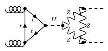
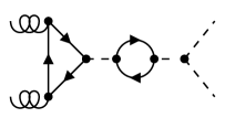
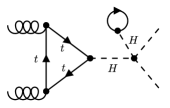
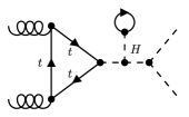
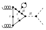
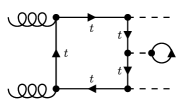
In this contribution we compute exact analytic results for the factorizable contribution to Higgs boson pair production in gluon fusion. Sample Feynman diagram are shown in Fig. 1. In the next section we provide details regarding the calculation, Section 3 deals with the renormalization and Section 4 discusses the results and provides a summary.
 |
 |
 |
 |
| class 1 | class 2 | class 3 | class 4 |
 |
 |
||
| class 5 | class 6 |
2 Technical details
For the generation of the Feynman amplitudes we use qgraf [6] and process them afterwards with tapir [7] and exp [8, 9]. We use the FORM-based [10] setup calc for the manipulation of the matrix algebra, the application of projectors, and the reduction to master integrals. In the following we provide more details regarding some of these elements.
The amplitude for the process (with ) is conveniently decomposed into two Lorentz structures
| (1) |
where and are adjoint colour indices and the Lorentz structures are given by
| (2) |
In this equation the following abbreviations have been introduced
| (3) |
where is the squared partonic centre-of-mass energy, and , are Mandelstam variables which fulfill , and the prefactor is given by
| (4) |
with , is Fermi’s constant and is the strong coupling constant evaluated at the renormalization scale . We define perturbative expansion of the form factors as
| (5) |
where is the fine structure constant.
Equation (1) defines the two form factors and . Note that the Feynman diagrams considered in this paper from class 1 to 4 in Fig. 1 only contribute to since only gets contributions from box diagrams. These diagrams all have at least one bridge connecting the initial and final states. In practice, only Higgs bosons serve as bridges. Note that diagrams with bosons or neutral Goldstone bosons do not contribute, as the vector coupling part vanishes due to the charge conjugation symmetry, and the axial coupling part vanishes due to the parity-even properties of the process. We will provide final results for the renormalized form factor in Feynman gauge. Note that the finite part of the renormalized factorizable form factor depends on and . They will drop out once also the non-factorizable contribution is added. This has been checked in Ref. [5] in the large- limit.
We classify the factorizable contribution into six groups which are shown in Fig. 1. Classes 5 and 6 contribute to the renormalization of the top quark mass and they cancel exactly if the top quark is renormalized on shell.111Note that box diagrams in class 6 provide contributions both to and . In our calculation the corresponding diagrams are included, however, to avoid confusion, we discard them in the final expressions provided in the ancillary file. The remaining diagrams can be classified according to the number of -channel Higgs boson propagators, and propagators without momentum flow, . The latter arise from diagrams with tadpoles.
-
•
class 1: single , no
-
•
class 2: double , no
-
•
class 3: single and single
-
•
class 4: double and single
As we will discuss in Section 3 these classes renormalize separately.
For the practical calculation one only has to consider one-loop integrals which are well known in the literature. However, it is important that in intermediate steps higher order terms are properly taken into account. Thus, in our calculation we refrain from using published packages since they are either targeted to the limit or the handling of higher order terms is not transparent. Rather, we define box-type integral families within our FORM setup with external momenta and . In our routines we even have although for the current application is sufficient. We use LiteRed [11] to generate generic reduction rules which we then convert to FORM code. This allows us to perform the reduction to master integrals within the calc setup in a fast and efficient way for general dimensional parameter .
After inserting explicit result for the one-loop tadpole contributions we can express our final result in terms of (products of) one-loop two- and three-point functions. More precisely, we have the term of two-point functions with squared external momentum , or . Both internal lines have the same mass, either or . Furthermore, there are two types of three-point functions. Both of them have the virtuality on one of the external legs and the other two are both either zero or . All three lines have again the same mass. The bare expression also contains the term of order of the three-point function with external momenta and internal top quark mass. As we will see in Section 3, this contribution cancels after renormalization.
In our final results, we introduce the following notation for these functions
| (6) |
where is the internal particle mass. These notations are quite standard and we have adopted them from LoopTools [13]. To clarify our convention and normalization, we provide the two-point and three-point functions including terms
| (7) |
where . As presented, the formula is valid for . It can be evaluated in other kinematical regions by proper analytic continuation taking into account .
3 Renormalization
The renormalization of the complete contribution (i.e. factorizable and non-factorizable) is discussed in Ref. [5] where it has successfully been applied in the large- limit. From the considerations in [5] it is straightforward to extract the following prescription which leads to a finite results for the factorizable contribution:
-
•
At LO we only consider the triangle diagram and renormalize the parameters associated to the Higgs propagator and trilinear coupling in the on-shell scheme. Here is the Higgs boson self-coupling, is the vacuum expectation value, is the Higgs boson mass. Note that the top-Yukawa coupling and top-mass are not renormalized.
-
•
In addition to the parameter renormalization we have to take into account the wave function renormalization of the external Higgs boson field. For the factorizable part half of this contribution is needed; the other half is needed for the non-factorizable contribution.
In practice, we use the relation
| (8) |
where is the weak mixing angle and . We use this relation between bare and renormalized parameters for where is the electric charge. Note that in all parts we retain all tadpole contributions from Higgs boson lines except those where the Higgs boson is attached to a top quark line. The latter contribution is closely related to the top quark mass renormalization in the non-factorizable contribution (see also discussion above).
The main results of this contribution are obtained in Feynman gauge. In principle, a calculation for generic gauge parameters ( and ) is possible but tedious since in that case different masses appear inside the loop functions. In Ref. [5] we have incorporated the and terms in the limits and have checked that in the sum of all contributions the gauge parameters drop out. In other kinematic limits we can proceed in a similar way.
4 Results and Summary
We present our final results in electronic form [12]. We introduce labels for each counterterm contribution such that the bare result is obtained if they are set to zero. Furthermore, there are labels for the four classes 1 to 4. Note that the introduced in Eq.(6) drops out after renormalization. For reference we provide in the following the one-loop triangle form factor up to
| (9) |
where is defined after Eq.(7). Note that our final expression only contains scalar functions and no tensor coefficient functions. The analytic results are well known and easy to evaluate numerically with packages like LoopTools [13], PackageX [14], Collier [15], OneLoop [16] and other packages. For a subset of our results involving top-Yukawa and Higgs self-coupling contributions, we have compared to Ref. [2] and found agreement.
To summarize, in these proceedings we present a further building block to the NLO electroweak corrections to the process : the complete factorizable contributions. We provide our results in a computer-readable file which makes an implementeation in a numerical code straightforward.
5 Acknowledgements
This research was supported by the Deutsche Forschungsgemeinschaft (DFG, German Research Foundation) under grant 396021762 — TRR 257 “Particle Physics Phenomenology after the Higgs Discovery” and has received funding from the European Research Council (ERC) under the European Union’s Horizon 2020 research and innovation programme grant agreement 101019620 (ERC Advanced Grant TOPUP). The work of JD is supported by the STFC Consolidated Grant ST/X000699/1. The authors thank G. Heinrich, S. P. Jones, M. Kerner, T. W. Stone and A. Vestner for sharing their unpublished results for comparisons.
References
- [1] H.-Y. Bi, L.-H. Huang, R.-J. Huang, Y.-Q. Ma and H.-M. Yu, Electroweak Corrections to Double Higgs Production at the LHC, Phys. Rev. Lett. 132 (2024) 231802 [2311.16963].
- [2] G. Heinrich, S. P. Jones, M. Kerner, T. W. Stone and A. Vestner Electroweak corrections to Higgs boson pair production: The top-Yukawa and self-coupling contributions, [2407.04653].
- [3] J. Davies, G. Mishima, K. Schönwald, M. Steinhauser and H. Zhang, Higgs boson contribution to the leading two-loop Yukawa corrections to gg → HH, JHEP 08 (2022) 259 [2207.02587].
- [4] M. Mühlleitner, J. Schlenk and M. Spira, Top-Yukawa-induced corrections to Higgs pair production, JHEP 10 (2022) 185 [2207.02524].
- [5] J. Davies, K. Schönwald, M. Steinhauser and H. Zhang, Next-to-leading order electroweak corrections to and in the large- limit, JHEP 10 (2023) 033 [2308.01355].
- [6] P. Nogueira, Automatic Feynman Graph Generation, J. Comput. Phys. 105 (1993) 279.
- [7] M. Gerlach, F. Herren and M. Lang, tapir: A tool for topologies, amplitudes, partial fraction decomposition and input for reductions, Comput. Phys. Commun. 282 (2023) 108544 [2201.05618].
- [8] R. Harlander, T. Seidensticker and M. Steinhauser, Complete corrections of Order alpha alpha-s to the decay of the Z boson into bottom quarks, Phys. Lett. B 426 (1998) 125 [hep-ph/9712228].
- [9] T. Seidensticker, Automatic application of successive asymptotic expansions of Feynman diagrams, in 6th International Workshop on New Computing Techniques in Physics Research: Software Engineering, Artificial Intelligence Neural Nets, Genetic Algorithms, Symbolic Algebra, Automatic Calculation, 5, 1999, hep-ph/9905298.
- [10] B. Ruijl, T. Ueda and J. Vermaseren, FORM version 4.2, 1707.06453.
- [11] R. N. Lee, Presenting LiteRed: a tool for the Loop InTEgrals REDuction, 1212.2685.
-
[12]
https://www.ttp.kit.edu/preprints/2024/ttp24-023/. - [13] T. Hahn and M. Perez-Victoria, Automatized one loop calculations in four-dimensions and D-dimensions, Comput. Phys. Commun. 118 (1999) 153 [hep-ph/9807565].
- [14] H. H. Patel, Package-X 2.0: A Mathematica package for the analytic calculation of one-loop integrals, Comput. Phys. Commun. 218 (2017) 66 [1612.00009].
- [15] A. Denner, S. Dittmaier and L. Hofer, Collier: a fortran-based Complex One-Loop LIbrary in Extended Regularizations, Comput. Phys. Commun. 212 (2017) 220 [1604.06792].
- [16] A. van Hameren, OneLOop: For the evaluation of one-loop scalar functions, Comput. Phys. Commun. 182 (2011) 2427 [1007.4716].