Probabilistic Shoenfield Machines

1 Abstract

This article provides the theoretical framework of Probabilistic Shoenfield Machines (PSMs), an extension of the classical Shoenfield Machine that models randomness in the computation process. PSMs are brought in contexts where deterministic computation is insufficient, such as randomized algorithms. By allowing transitions to multiple possible states with certain probabilities, PSMs can solve problems and make decisions based on probabilistic outcomes, hence expanding the variety of possible computations. We provide an overview of PSMs, detailing their formal definitions as well as the computation mechanism and their equivalence with Non-deterministic Shoenfield Machines (NSM).

2 Introduction

Theoretical computer science is rich with different models that were created to formalize and understand the limits of computation. Among these, the Deterministic Shoenfield Machine (DSM) turns out to be the simplest one, providing a fundamental framework to recognize whether a function is computable or not. However, as the work in that matter progressed, the necessity occurred to extend this classical model to capture a broader spectrum of computational phenomena, creating the probabilistic models of computation. One of these significant extensions, which is provided in this paper, is the Probabilistic Shoenfield Machine (PSM). In this article, we discuss what PSM is, stating its formal definition and mechanism of computation.

A Probabilistic Shoenfield Machine is a type of the DSM that models the elements of randomness in its computation process. This model is particularly pertinent in contexts where deterministic computation may not be applicable, such as in the case of randomized algorithms, cryptographic protocols, and probabilistic analysis. Unlike a classical Shoenfield Machine, which computes along a single path defined by its deterministic transition function, a PSM can transition into multiple possible states with different probabilities. This probabilistic behavior allows PSMs to solve problems and make decisions based on different outcomes, thus adding to the spectrum of things that can be computed.

The concept of PSMs not only broadens the number of theoretical means of computation but also has practical implications. For example, probabilistic algorithms, which are exploited by many modern technologies, rely on the probabilistic computation schema to achieve faster or more efficient solutions compared to their deterministic computations. Moreover, the study of such models interplays with other branches of theoretical computer science.

By extending the computational potential of traditional Shoenfield Machines to include probabilistic transitions, PSMs represent an advancement in the theoretical understanding of computation. Through this study, we hope to present aspects of probabilistic computation and its impact on the development of the study of computational matter.

The following document provides introductions of Non-deterministic Shoenfield Machines (NSM) and Probabilistic Shoenfield Machines (PSM), both based on Deterministic Shoenfield Machines DSN, as a formal model of computation. The document begins with a detailed definition of DSM, outlining its components and the Representation of its computation. It further shows a short introduction of NSM and establishes its computational equivalence with DSM. Next, the PSM is introduced, and its equivalence to DSM is discussed.

3 Deterministic Shoenfield Machines

A Deterministic Shoenfield Machine (DSM) is a formal model of computation introduced by J. R. Shoenfield in [1] and then even simplified by Y. L. Yershov in [2]. We will start with Yershow’s definition of DSM. In the paper, we exploit the fact that it was shown in this paper that the computation power of the model is equivalent to the power of Turing Machines.

3.1 Definition of DSM

A Deterministic Shoenfield Machine is a computation model composed of:

• An infinite set of registers enumerated by numbers $0,1,2\dotso$. Each register $R_{i}$ is a memory cell containing a natural number. The number in a particular register may change its value during the computation. During the computation, the machine uses only a finite number of registers. The purpose of registers is to store the data (natural numbers).

• An instruction counter. It is a memory cell containing a natural number at any time. The number points to the index number of the instruction within the program which is supposed to be executed next. At the beginning of the computation, it contains $0$.

• A program is placed in a separate part of the machine’s memory. It is a finite list of instructions enumerated from $0$ to some natural $n$. During the computation, the program does not change.

The program is written down before running the DSM, registers are filled with input data, and the instruction counter is set to 0. The machine executes the instruction at one step, the index of which is present in the instruction counter. The machine stops its computation only if the instruction counterpoints to an instruction number that does not exist in the program. It is also possible that a machine never halts.

There are only two types of instructions:

• $INC\ i$ - during the execution of this instruction, the machine increments the value stored in the $i$-th register and the instruction counter by one. Then, the machine continues to the next step.

• $DEC\ i,n$ - if at the beginning of the execution of this instruction, the value stored in the $i$-th register is greater than 0, then the machine decrements this value by one and sets the instruction counter to $n$. Otherwise, if the value stored in the $i$-th register equals 0, then the machine increments the instruction counter by one.

3.2 Representation of computation of a DSM

A temporary configuration of a particular DSM may be represented by two pieces of data:

• current values stored in all of the registers,

• current value of the instruction counter.

Let us note that we may represent a computation of a particular DSM as a descending chain (possibly infinite) where the top element represents the initial configuration. The direct descendant of the top element is the configuration obtained after executing the program instruction which is present in line number 0 (since, at the beginning of the computation, the instruction counter value is 0). The following configurations in the chain are constructed as resulting configurations of executing the instruction pointed by an instruction counter on the preceding configuration.

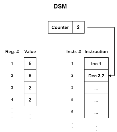
Figure 1: This figure represents a Deterministic Shoenfield Machine (DSM). The machine has a counter set to 2, which points to the next instruction. Multiple registers hold integer values: Register 1 has 5, Register 2 has 6, Register 3 has 2, and Register 4 has 2. The instruction list includes operations such as Inc 1 (increment Register 1) and Dec 3, 2 (decrement Register 3 and set the counter to 2 if the result is zero). The current instruction to be executed is Dec 3, 2.

4 Non-deterministic Shoenfield Machines

In this section, we introduce Non-deterministic Shoenfield Machines (NSM), and we show their computational equivalence with DSM.

4.1 Definition of NSM

A Non-deterministic Shoenfield Machine (NSM) is a computation model composed of:

• An infinite array of registers, as in the case of DSM.

• An instruction counter. The instruction counter is set to 0 at the beginning of the computation.

• A program is placed in a separate memory part of the machine as in the case of DSM, however, each program line contains a finite number of instructions.

The program is written down before running the NSM, registers are filled with the input data, and the instruction counter is set to 0. At one step, the machine executes the program line, which is pointed by the instruction counter. If there is more than one instruction in the cell, the machine replicates the current configuration of the registers, counter and the program, creating as many copies of the machine as the number of instructions in the current program line. Then, the machine executes one instruction from the line separately in each of the copy and updates the instruction counters accordingly to the instruction executed. The computation in each cell proceeds separately. The machine halts if all of the submachines created halt. In the other case, it works without halting.

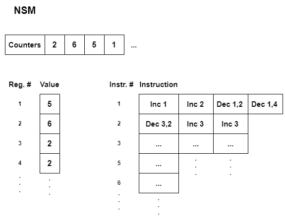
Figure 2: This diagram represents a Non-deterministic Shoenfield Machine (NSM). The machine consists of multiple counters (2, 6, 5, 1, …), which point to possible next instructions. Registers hold integer values: Register 1 has 5, Register 2 has 6, Register 3 has 2, and Register 4 has 2. The instruction list includes operations such as Inc 1, Inc 2, Dec 1, 2, Dec 1, 4, and Dec 3, 2. This machine can follow different execution paths due to multiple counters pointing to different instructions.

4.1.1 Theorem

Every NSM is equivalent with some DSM.

Proof

Let $M$ be a NSM. Firstly, we present a procedure of building a tree $T$ of the computation of $M$. Secondly, we show that every path from the root of $T$ to any of its leaves represents a finite computation of a DSM. If some path is infinite, it represents an infinite computation of some DSM.

4.2 Building up the computation tree $T$ of NSM $M$

1) Let $k_{0}$ be an initial configuration of registers of machine $M$. Let $n_{0}$ be an initial instruction counter value of machine $M$. In the root of $T$ we store information about $k_{0}$ and $n_{0}$:

$$k_{0}|n_{0}:=w_{0}.$$

2) Now, let us assume that our starting node is:

$$w_{i}=k_{i}|n_{i}.$$

The succeeding nodes of $T$ are constructed inductively as follows:

A) If $n_{i}$ points at the line of program which contains only one instruction $c$ then the only descendant of the node $w_{i}$ is the node $w_{i+1}=k_{i+1}|n_{i+1}$, where $k_{i+1}$ is the configuration of registers obtained after execution of $c$ on configuration $k_{i}$. Further, $n_{i+1}$ is the value of the instruction counter we obtain after executing $c$, assuming that the previous value of the instruction counter was $n_{i}$.

B) If $n_{i}$ points at the line of program which contains several instructions $c_{1},c_{2},\dotso,c_{m}$ then there are created $m$ descendants of the node $w_{i}$:

$$w^{1}_{i+1}=k^{1}_{i+1}|n^{1}_{i+1},w^{2}_{i+1}=k^{2}_{i+1}|n^{2}_{i+1},\dotso,w^{m}_{i+1}=k^{m}_{i+1}|n^{m}_{i+1},$$

where $w^{a}_{i+1}$ is obtained by executing $c_{a}$ on the configuration $w_{i}$ in the same manner as in A).

According to the rules of building the tree $T$, there are two options for how each of the branches of the tree may look like:

• The path may end with a final configuration, which we call a leaf node.

• The path may be infinite.

Let us notice that every path from the root of $T$, which ends in a leaf $w_{n}$, is equivalent to the computation of some DSM. Based on transitions between each node and its direct descendant in the particular path, we can recover instructions executed along the path. That allows us to recover from the program.

In the case of the infinite path, we can also recover a program executed along the path. As long as the initial program of $M$ is finite, the one executed in the path must be finite and looped so it executes infinitely.

If the path in $T$ is finite then, by [3, Theorem 34] it is equivalent to a computation of some partial recursive function and hence, such a path is also equivalent to some DSM for which the input $w_{0}$ results with a defined value.

If the path in $T$ is infinite, then, by the same theorem from [3], it is equivalent to a computation of some DSM for which the input $w_{0}$ results with infinite computation. $\blacksquare$

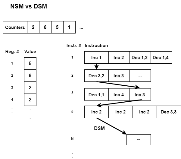
Figure 3: This diagram compares a Non-deterministic Shoenfield Machine (NSM) and a Deterministic Shoenfield Machine (DSM). The NSM has multiple counters (2, 6, 5, 1, …) pointing to possible next instructions, with registers holding values 5, 6, 2, and 2. Instructions include operations such as Inc 1, Dec 3,2, and Dec 1,2, with arrows showing possible transitions. The DSM follows a single deterministic path between instructions.

That equates us to NSM and DSM.

5 Probabilistic Shoenfield Machines

In this section, we introduce Probabilistic Shoenfield Machines (PSM), and we show their computational equivalence with DSM (NSM, TM). By design, the probabilistic Shoenfield machine is a development of the non-deterministic Shoenfield machine, where the choice of transition between specific states is made on the basis of a particular probability distribution.

5.1 Definition of PSM

• An infinite array of cells containing an infinite set of registers, as in the case of DSM and NSM.

• An infinite array of instruction counters. The first instruction counter is set to 0 at the beginning of the computation, while the value of the others is set to blank.

• A program is placed in a separate memory part of the machine as in the case of DSM and NSM. Each program line contains a finite number of instructions.

• A non-uniform oracle is a mechanism that generates random values from a specified set, where each value has an assigned probability. In the context of the defined machine with $n$ instructions in each row, selects an instruction based on a given set of probabilities $\{p_{1},p_{2},\ldots,p_{n}\}$, where $\sum_{i=1}^{n}p_{i}=1$ and $i$ is the number of instructions in the line.

• The execution of a given instruction in a line is done with the selected probability $p_{i}$.

Analogous to NSM, before the PSM is run, the program is written, the registers in the first cell of the array are filled with input data, and the counter of the first instruction is set to 0. The machine executes a program line in one step indicated by the instruction counter. However, in the case of PSM, the execution of a given instruction in a line is done with the probability $p_{i}$. The sum of all right-likelihoods in a line, $\sum_{i=1}^{n}p_{i}=1$, where $i$ is the instruction number, and $n$ is the number of instruction in line. The $p_{i}$ probabilities are not necessarily equal.

It is worth noting that the execution of each instruction with a certain probability is the probability of a given configuration of registers after the operation.

In contrast to the NSM, the machine can only execute one instruction per line with a probability of $p_{i}$.

The probability of moving to any state beyond the current one is zero if and only if it is an accepting state (final state).

5.2 Equivalence between PSM and NSM

The equivalence between NSM and PSM is due to the fact that the computation in PSM is the same as in NSM, and a particular instruction is selected with probability $p_{i}$, where the probability of selecting all instructions in a line adds up to 1. From this, the equivalence between PSM and NSM is shown.

5.3 Bulding up the computation path P of PSM

Unlike NSM, in the case of PSM, we are dealing with a path P in the tree.

1) Let $k_{0}$ be an initial configuration of registers of machine $M$. Let $n_{0}$ be an initial instruction counter value of machine $M$. In the first row of $P$ we store information about $k_{0}$ and $n_{0}$:

$$k_{0}|n_{0}:=w_{0}.$$

2) Now, let us assume that our starting node or path is:

$$w_{i}=k_{i}|n_{i}.$$

The succeeding nodes of $P$ are constructed inductively as follows:

A) If $n_{i}$ points at the line of the program which contains only one instruction $c$, whose execution probability is 1, then, as with NSM, the only descendant of the node $w_{i}$ is the node $w_{i+1}=k_{i+1}|n_{i+1}$, where $k_{i+1}$ is the configuration of registers obtained after execution of $c$ on configuration $k_{i}$. Further, $n_{i+1}$ is the value of the instruction counter we obtain after executing $c$, assuming that the previous value of the instruction counter was $n_{i}$.

B) If $n_{i}$ points to a program line that contains several instructions $c_{1},c_{2},\dotso,c_{m}$, then one of them is executed with probability $p_{i}$. In this case, however, unlike NSM, an execution path is created. Thus, one descendant of the node $w_{i}$ is created:

$$w^{a}_{i+1}=k^{a}_{i+1}|n^{a}_{i+1},$$

where $w^{a}_{i+1}$ is obtained by executing $c_{a}$ on the configuration $w_{i}$ in the same manner as in A).

Thus, with probability $p_{i}$, one descendant of node $w_{i}$ is created. According to the presented $P$ path construction rules, there are two options for the appearance of each branch of the tree:

• A path can end with a final configuration, called leaf node.

• The path can be infinite.

By analogy with NSM, let us note that each path from the root $P$ that ends in the leaf $w_{n}$ is equivalent to computing some DSM. We can recover the instructions executed along that path based on the transitions between each node and its direct descendant in a given path.

The probability of executing an instruction $w^{a}_{i+1}$, which is one of the descendants of node $w_{i}$ in the Probabilistic Shoenfield Machine (PSM) model, depends on the probability of selecting a particular instruction $c_{a}$ at a given program stage.

The single path of computation in PSM is equivalent to DSM, and therefore, the same principles apply as we discussed in the section on DSM. The only difference is that it is executed with a probability equal to the product of the probabilities of the drawn instructions.

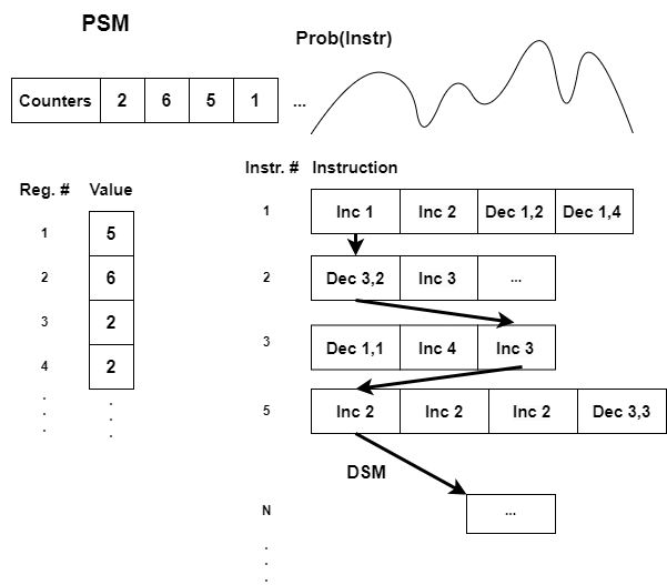
Figure 4: The Probabilistic Shoenfield Machine (PSM). In this case, the machine has multiple counters (2, 6, 5, 1, …) indicating possible next instructions, with registers holding values 5, 6, 2, and 2. Instructions include operations such as Inc 1, Dec 3,2, and Dec 1,2, with arrows showing possible transitions. A graph represents the probabilities of different instructions. The DSM follows a single deterministic path between instructions.

5.4 Equivalnce between DSM and PSM

When we use DSM to simulate a PSM machine, a deterministic DSM machine can simulate PSM using a pseudorandom number generator to mimic probabilistic choices. This simulation involves encoding the state of the random number generator into a deterministic machine. The key challenge here is the overhead associated with deterministic randomness management.

In the reverse case, when we simulate a deterministic DSM machine using PSM, the deterministic behavior is a special case of probabilistic behavior (where the probability is 0 or 1). In this situation, PSM can directly simulate any deterministic machine without additional complexity.

6 Aplications

6.1 Potential Applications for Probabilistic Computations

Computer science applications cover areas where something more than classical computational models, such as the classical Turing Machine (TM), may be required. Modeling computation with a Probabilistic Turing Machine (PTM) may be more appropriate because the PTM considers elements of randomness, which is particularly important in environments where deterministic operating conditions cannot be guaranteed.

Such an environment is, for example, space and the equipment operating there, which must cope with intense radiation. Crossing Jupiter’s radiation belts exposes hardware and algorithms to high radiation levels, which can disrupt traditional calculations. Under such conditions, the PTM can better reflect the natural operating environment, considering the effects of radiation on computational processes.

Under such conditions, the PTM may be better suited to study computing behavior in considerable measure by approximating the radiation-related conditions there.

A very similar situation exists in the case of nuclear remediation robots.

Even in everyday computations involving many individual operations, such as calculations of $\pi$ with record precision, cosmic radiation can introduce unpredictable disturbances that influence the results. Using a Probabilistic Turing Machine (PTM) is invaluable in such cases. PTMs can account for these unpredictable disturbances, leading to more reliable outcomes. This versatility of PTMs in accounting for unpredictable factors in everyday computations is a crucial aspect of their application. In summary, the Probabilistic Turing Machine and, per analogy, the Probabilistic Shoenfield Machine could find applications in many areas where classical computational models, like PTM, may not meet the challenges posed by unpredictable external factors. By incorporating elements of randomness, PTM allows for more realistic and reliable modeling of computational processes under challenging conditions. [5]

6.2 Potential Applications analog to PTM

Meanwhile, PTMs, as a formalism, have well-established and well-known applications. However, by analogy and equivalence between PTMs and PSMs, we can expect them to perform well in many similar applications and areas, for example, Generating random numbers and keys [6] and Probabilistic encryption schemes [6].

As another example, we can consider randomized algorithms, where PSM can provide a theoretical basis for randomized algorithms that use random choices to solve problems more efficiently than deterministic algorithms. In this case, examples include New methods for primality testing, [4], and polynomial identity testing [4].

Particularly promising seems to be PSM’s potential ability to model complex randomness in systems such as quantum systems, neural networks, or complex biological processes, for example.

7 Conclusions

In this work, we have introduced two new formalisms based on the register machines, the classical Shoenfield Machines: the Non-deterministic Shoenfield Machine and the Probabilistic Shoenfield Machine.

References

- [1] J. R. Shoenfield, Recursion Theory, Springer-Verlag, Berlin, 1993.
- [2] Y. L. Yershov, Теория нумераций, Nauka, Moscow, 1977.
- [3] Н. Т. Когабаев, Лекции по теории алгоритмов, Novosibirsk State University, Novosibirsk, 2009.
- [4] Arora, Sanjeev, and Boaz Barak. Computational complexity: a modern approach Cambridge University Press, 2009.
- [5] Draeger, J. Universal, Nondeterministic, and Probabilistic Turing Machines
- [6] Klingler, Lee, Rainer Steinwandt, and Dominique Unruh. On using probabilistic Turing machines to model participants in cryptographic protocols Theoretical Computer Science 501 (2013): 49-51.