Preparation of Schrödinger cat quantum state using parametric down-conversion interaction

Abstract

The Schrödinger cat state is important in quantum optics because of its non-Gaussian properties. This paper proposes the use of degenerate parametric scattering and measurement of the number of photons in the pump mode to conditionally prepare the Schrödinger cat state. This method ensures the preparation of SC in systems with weak parametric non-linear interaction. Comparison with the existing whispering mode gallery microresonator from lithium niobate indicates the possible applicability of this method.

I Introduction

Preparation of non-Gaussian states is an important task in quantum optics. One of the most well known type of the non-Gaussian states are the Schrödinger cat (SC) states. They can be used, in particular, in coherent state quantum computing [1, 2, 3, 4, 5] and in the optical interferometry [6, 7, 8, 9, 10].

The “mainstream” method of the SC states preparation is based in photon subtraction and conditional measurement, see Refs. [11, 12, 13, 14, 15, 16] and the review [17]. The values of SC state amplitudes up to $\alpha\sim 2$ were demonstrated using this method. The recent esimates [18, 19] show that it allows to prepare SC states with the amplitudes $\alpha\gtrsim 4$ and fidelity exceeding 99%

It was shown in the works [20, 21] that much more bright (multli-photon) quantum states having the characteristic SC-like two maxima shape can be generated using the second order optical nonlinearity described by the Hamiltonian

$$\hat{H}_{2}=\hbar\gamma\left(\hat{a}^{2}\hat{b}^{\dagger}+\hat{a}^{\dagger 2}\hat{b}\right),$$ (1)

where $\gamma$ is the parametric interaction coefficient, $\hat{a}$ and $\hat{b}$ are the annihilation operator of two optical modes of with the frequencies $\omega$ (the signal one) and $2\omega$ (the pump one). Depending on the initial conditions, this Hamitonian could describes nonlinear processes of the second harmonic generation or the degenerate parametric down-conversion. It is the second one is responsible for the SC-like state generation in the signal mode.

In both those works, joint unitary evolution of the two modes was analyzed numerically. In Ref. [20], evolution of the Husimi quasi-probability function of the signal mode was explored. However, in the general case, tracing out the pump mode gives a mixed state of the signal one. Therefore, this approach can not be considered as the optimal.

In our paper, we propose a conditional preparation procedure based on the heralding measurement of the photon number in the pump mode. The paper is organized as follows. In Sec. II we review the convenient representation of the two-mode quantum states that was introduced in Refs. [20, 21] and that we use in our numerical calculations here. In Sec. III we discuss the unconditional evolution of our system. In Sec. IV we introduce the conditional preparation procedure and show that in principle, it allows to prepare the SC states with the fidelity approaching one. In Sec. V we discuss the practical feasibility of implementation of the proposed procedure using the whispering gallery mode microresonators.

II Numerical calculation of evolution

An analytical solution of the Shrödinger equation for Hamiltonian (1)

$$i\hbar\frac{\partial|{\Psi(t)}\rangle}{\partial t}=\hat{H}_{2}|{\Psi(t)}\rangle$$ (2)

is unknown, therefore, we use the numerical solution in this paper. The straightforward approach in this case is to use the two-dimensional Fock basis

$$\{|{n}\rangle_{s}\otimes|{n}\rangle_{p}\}\,,$$ (3)

where $|{n}\rangle_{s}$, $|{n}\rangle_{p}$ are the energy eigenstates of the signal and pump modes. However, numerical calculation using this representation requires very significant computational resources.

At the same time, note that the sum energy of the two modes

$$\hat{H}_{0}=\hbar\omega_{0}(\hat{a}^{\dagger}\hat{a}+2\hat{b}^{\dagger}\hat{b})$$ (4)

commutes with the Hamiltonian (1). This feature allows to represent $\hat{H}_{2}$ as follows:

$$\hat{H}_{2}=\hbar\gamma\sum_{N=0}^{\infty}\sum_{k,k^{\prime}=0}^{[N/2]}|{N-2k}\rangle_{s}\otimes|{k}\rangle_{p}H^{N}_{kk^{\prime}}\,{}_{s}\!\langle{N-2k^{\prime}}|\otimes{}_{p}\!\langle{k^{\prime}}|\,,$$ (5)

where […] denote integer part of number. The matrices $H^{N}_{kk^{\prime}}$ have the following tri-diagonal form:

$$\|H^{N}_{kk^{\prime}}\|=\begin{bmatrix}0&c_{0}^{N}&0&\dots&0&0\\ c_{0}^{N}&0&c_{1}^{N}&\dots&0&0\\ 0&c_{1}^{N}&0&\dots&0&0\\ \vdots&\vdots&\vdots&\ddots&c_{\left[\frac{N}{2}\right]-2}^{N}&0\\ 0&0&0&c_{\left[\frac{N}{2}\right]-2}^{N}&0&c_{\left[\frac{N}{2}\right]-1}^{N}\\ 0&0&0&0&c_{\left[\frac{N}{2}\right]-1}^{N}&0\\ \end{bmatrix},$$ (6)

with

$$c^{N}_{k}=\sqrt{(k+1)(N-2k)(N-2k-1)}\,,$$ (7)

see Refs. [20, 21]. This “semi-diagonalized” representation significantly reduces the requirements for computational resources.

Numerical methods for finding the eigenvectors of tridiagonal matrices are well developed. Let $\bigl{\{}\chi_{k}^{Nj}\bigr{\}}$, with $j=0\dots\left[\frac{N}{2}\right]$, be these eigenvectors, and $\lambda^{Nj}$ – the corresponding eigenvalues. It is easy to see that in this case, the eigenstates of the Hamiltonian $\hat{H}_{2}$ are equal to

$$|{\chi^{Nj}}\rangle=\sum_{k=0}^{\left[\frac{N}{2}\right]}\chi_{k}^{Nj}|{N-2k}\rangle_{s}\otimes|{k}\rangle_{p}$$ (8)

and the corresponding eigenvalues — to $\hbar\gamma\lambda^{Nj}$.

Let $|{\Psi}\rangle$ be the initial quantum state of our system. Using the basis $\{|{\chi^{Nj}}\rangle\}$, it can be presented as follows:

$$|{\Psi}\rangle=\sum_{N=0}^{\infty}\sum_{j=0}^{[N/2]}\Psi^{Nj}|{\chi^{Nj}}\rangle\,.$$ (9)

Its time evolution is described by the following equation:

$$|{\Psi(t)}\rangle=e^{-i\hat{H}_{2}t/\hbar}|{\Psi}\rangle=\sum_{N=0}^{N=\infty}\sum_{j=0}^{[N/2]}e^{-i\tau\lambda^{Nj}}|{\Psi^{Nj}}\rangle\,,$$ (10)

where

$$\tau=\gamma t$$ (11)

is the normalized time.

III Unconditional evolution

Suppose that initially the pump mode is prepared in the coherent quantum state $|{\beta}\rangle_{p}$ and the signal mode — in the vacuum state $|{0}\rangle_{s}$. In Fig. 1, the mean values of the normalized energy of the signal mode $\langle\hat{n}_{s}\rangle$ and the pump one $2\langle\hat{n}_{p}\rangle$, calculated using the method considered in Sec. II, are plotted as the function of the normalized time $\tau$ for the initial photon number in the pump mode $\langle\hat{n}_{p}\rangle=25$. In addition, the sum mean energy $\langle\hat{n}_{s}\rangle+2\langle\hat{n}_{p}\rangle$ is also shown. Energy remains constant, since the total energy operator $\hat{H}_{0}$ and the Hamiltonian $\hat{H}_{2}$ commute.

This plot clearly shows the interplay of the degenerate parametric down conversion process (which transfers the energy from the pump mode to the signal one) and the second harmonic generation one (which transfers the energy in the opposite direction). It is natural to expect that the maximums of $\langle\hat{n}_{s}\rangle$ correspond to the non-trivial non-Gaussian quantum states of the signal mode. This conclusion is supported also by the Figs. 1 and 4 of the paper [20].

In Fig. 2, the probability distribution for the photon number in the signal mode is shown. Similar to the “even” SC state

$$|{\psi_{\rm cat}}\rangle=\frac{1}{\sqrt{K}}\Big{(}|{\alpha}\rangle+|{-\alpha}\rangle\Big{)},$$ (12)

where $K$ is the normalization factor, the probabilities of the odd photon numbers are equal to zero, and the part of the distribution with the photon numbers above the mean value resembles the SC one. Unfortunately, this is not the case for the small values of $n_{s}$.

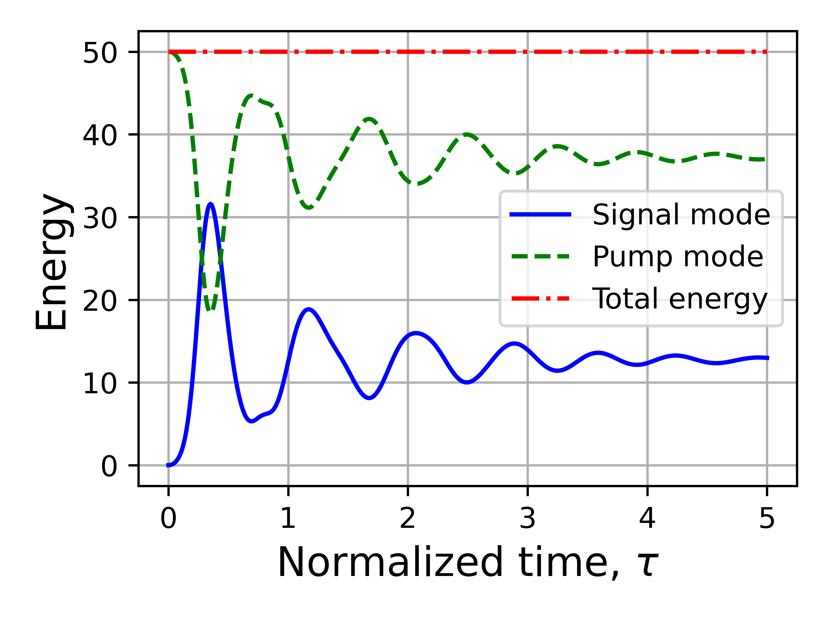
Figure 1: Blue solid: normalized mean energy of the signal mode $\langle\hat{n}_{s}\rangle$; green dashed line: normalized mean energy of the pump mode $2\langle\hat{n}_{p}\rangle$; red dash-dot line: the sum mean energy. The initial photon number in the pump mode $\langle\hat{n}_{p}\rangle=25$

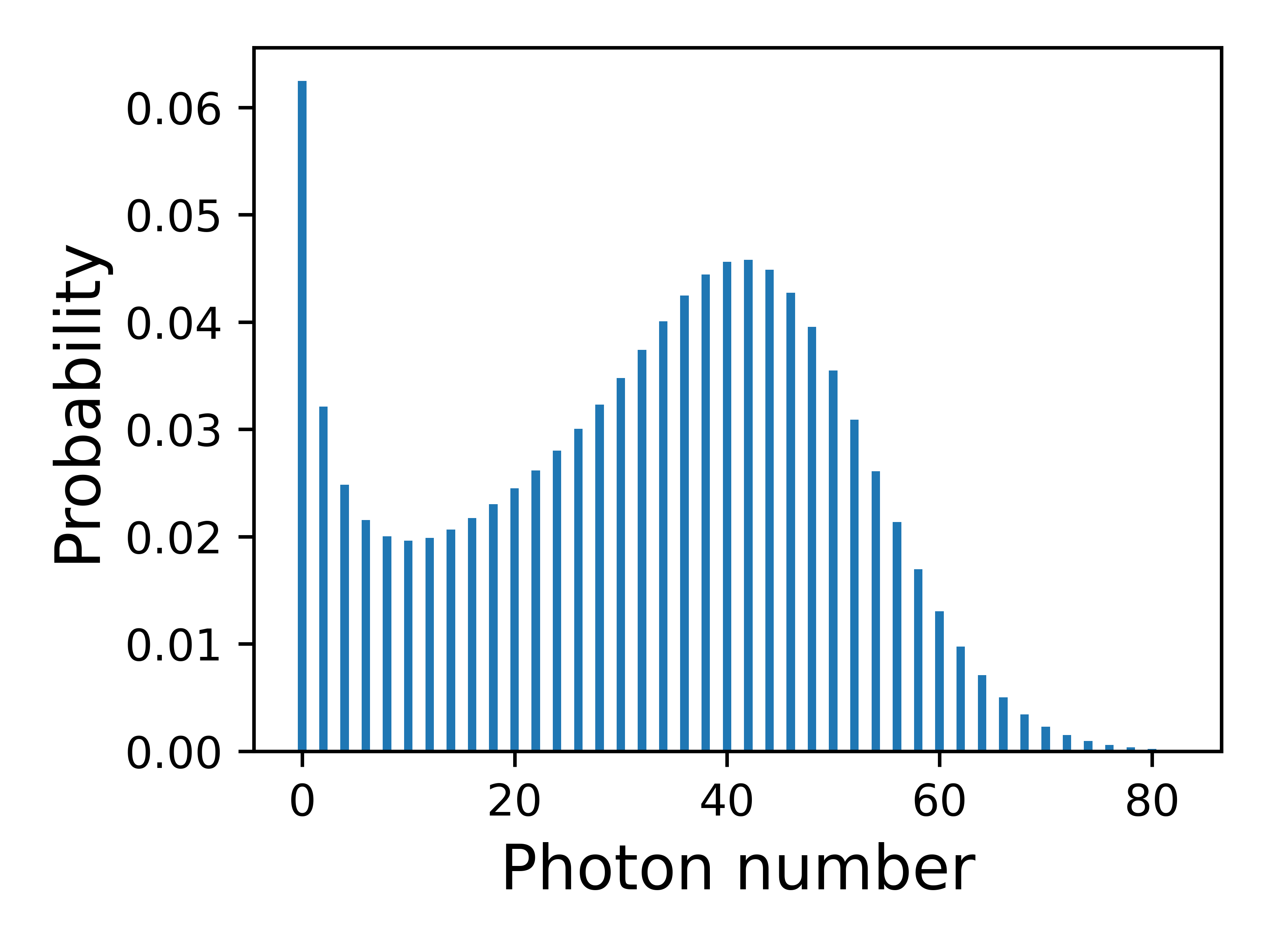
Figure 2: Probability distribution for the photon number in the signal mode at the optimal moment of time, showing the even statistics. The initial photon number in the pump mode $\langle\hat{n}_{p}\rangle=25$.

IV Conditional preparation of Schrödinger cat state

Suppose that at some moment of normalized time $\tau_{\rm opt}$, the photon number $\hat{n}_{p}$ in the pump mode is measured. Suppose also that we are interested only in the events where the value $\hat{n}_{p}=0$ is obtained. The schematic diagram of this procedure is shown in Fig. 3.

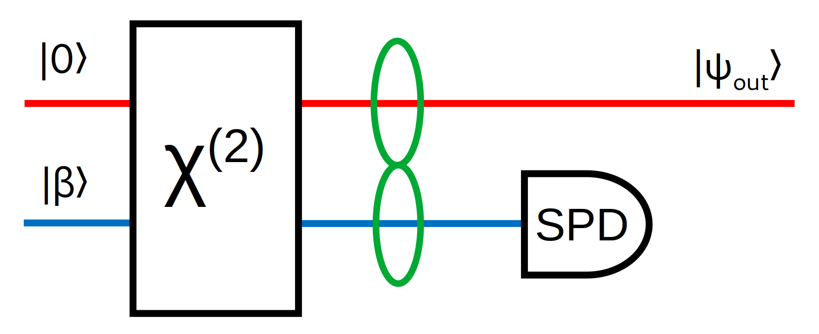
Figure 3: The scheme of the conditional preparation of the SC state. Red line – signal mode, blue line – pump mode. SPD – single photon detector.

As a result, the joint state of our two-mode system reduces to the separable one

$$|{\Psi}\rangle=|{0}\rangle_{p}\otimes|{\psi_{\rm out}}\rangle\,,$$ (13)

where $|{\psi_{\rm out}}\rangle$ is the resulting quantum state of the signal mode alone.

We assume that the moment of normalized time $\tau_{\rm opt}$ corresponds to the maximum of the probability $p_{0}$ of measuring zero photons in the pump mode. In Fig. 4, this probability is plotted as a function of the normalized interaction time $\tau$. The value of this time decreases with the increase of the initial coherent state amplitude in the pump mode $\beta$. This dependence can be approximated as follows:

$$\tau_{\rm opt}\approx\frac{b_{t}}{(1+c_{t}\beta)^{d_{t}}}$$ (14)

where $b_{t}\approx 1.337$, $c_{t}=0.791$, and $d_{t}\approx 0.850$.

Dependence of $p_{0}$ on $\beta$ can be approximated by the following function:

$$p_{0}\approx\frac{b_{p}}{(1+c_{p}\beta)^{d_{p}}}$$ (15)

where $b_{p}\approx 5.939$, $c_{p}\approx 5.072$, $d_{p}=0.995$.

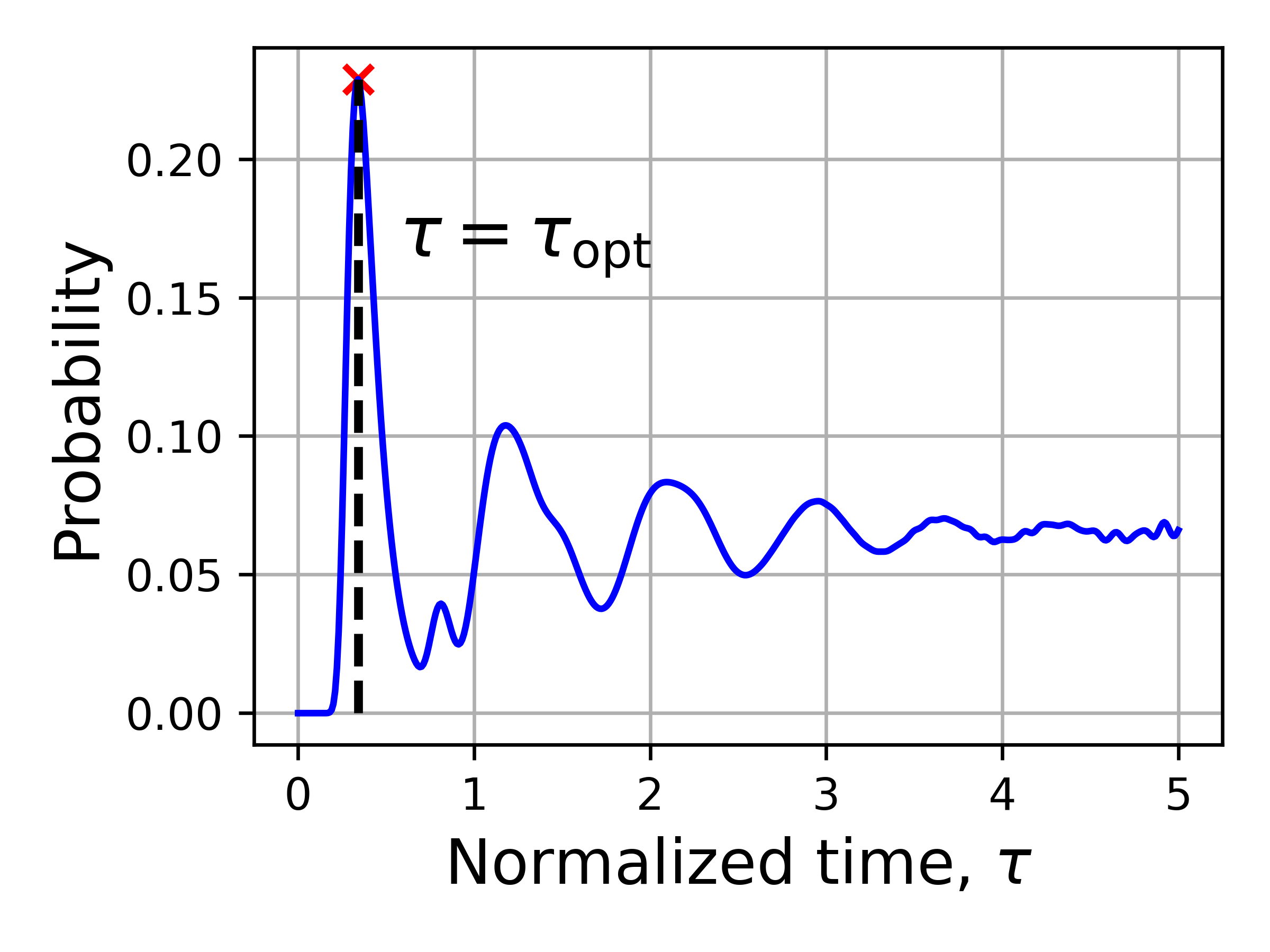
Figure 4: Dependence of the probability to measure zero photons in the pump mode on the interaction time. The initial photon number in the pump mode $\langle\hat{n}_{p}\rangle=25$.

In Fig. 5, the Wigner function of the resulting state $|{\psi_{\rm out}}\rangle$ is shown. It is easy to note that it strongly resembles the Wigner function of the squeezed and rotated by $-\pi/4$ SC state.

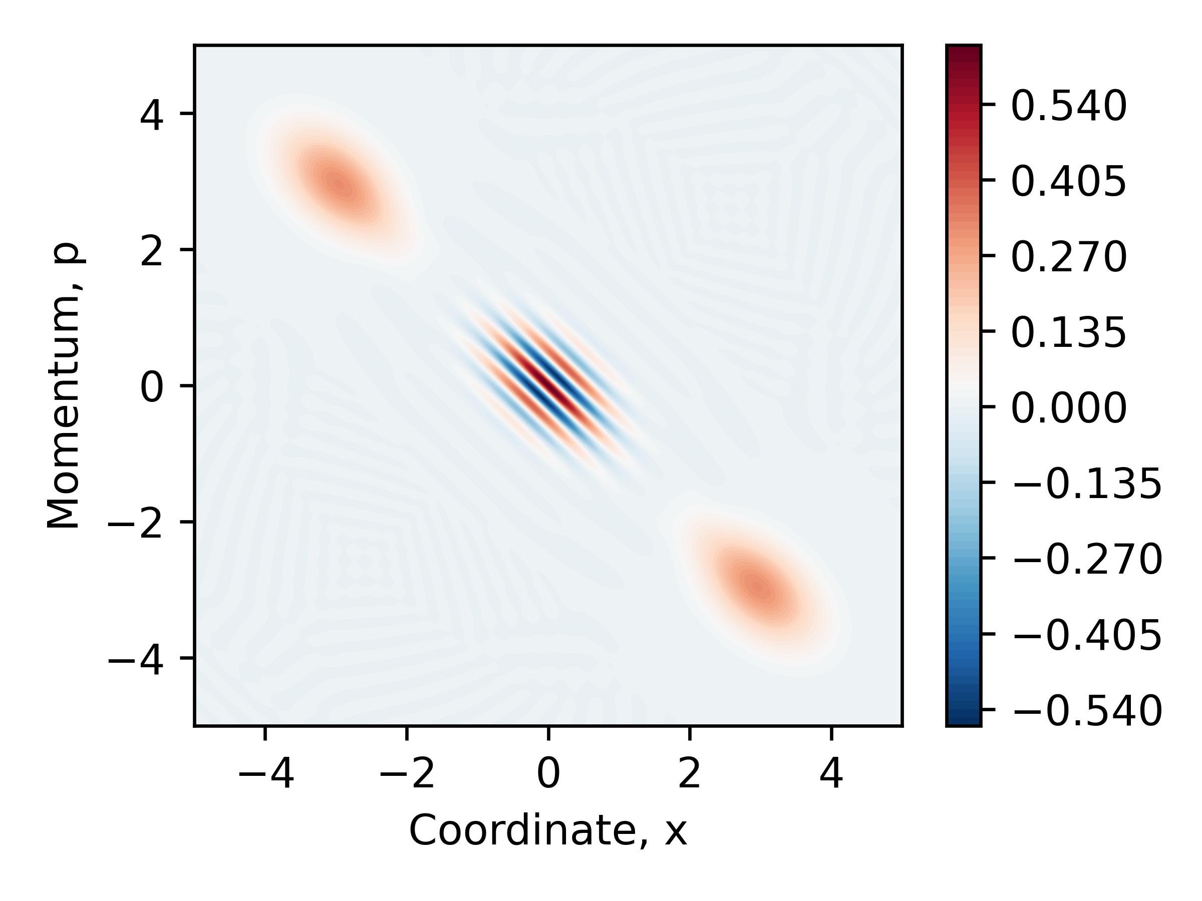
Figure 5: Wigner function of the output state $|{\psi_{\rm out}}\rangle$ at the optimal time $\tau_{\rm opt}$. $\beta=3,\,\alpha\approx 3\sqrt{2}$

As the quantitative measure of similarity of the obtained quantum state to the squeezed SC one, we consider the fidelity

$$F=|\langle\psi_{\rm out}|\hat{R}(-\pi/4)\hat{S}(r)|{\psi_{\rm cat}}\rangle\rangle|^{2}\,,$$ (16)

where $|{\psi_{\rm cat}}\rangle$ is the cat state (12), $\hat{R}$ is the unitary rotation operator, $\hat{S}(z)=\exp\left(\frac{1}{2}(z^{*}\hat{a}^{2}-z\hat{a}^{\dagger 2})\right)$ is the squeeze operator, and $r\in\mathbb{R}$ is the squeeze factor.

The optimal value of the squeeze parameter that provide the best fidelity can be approximated as follows:

$$r\approx a_{r}+\frac{b_{r}}{(1+c_{r}\beta)^{d_{r}}}\,,$$ (17)

where $a_{r}\approx-0.346$, $b_{r}\approx 0.141$, $c_{r}\approx 0.125$ and $d_{r}=2.395$.

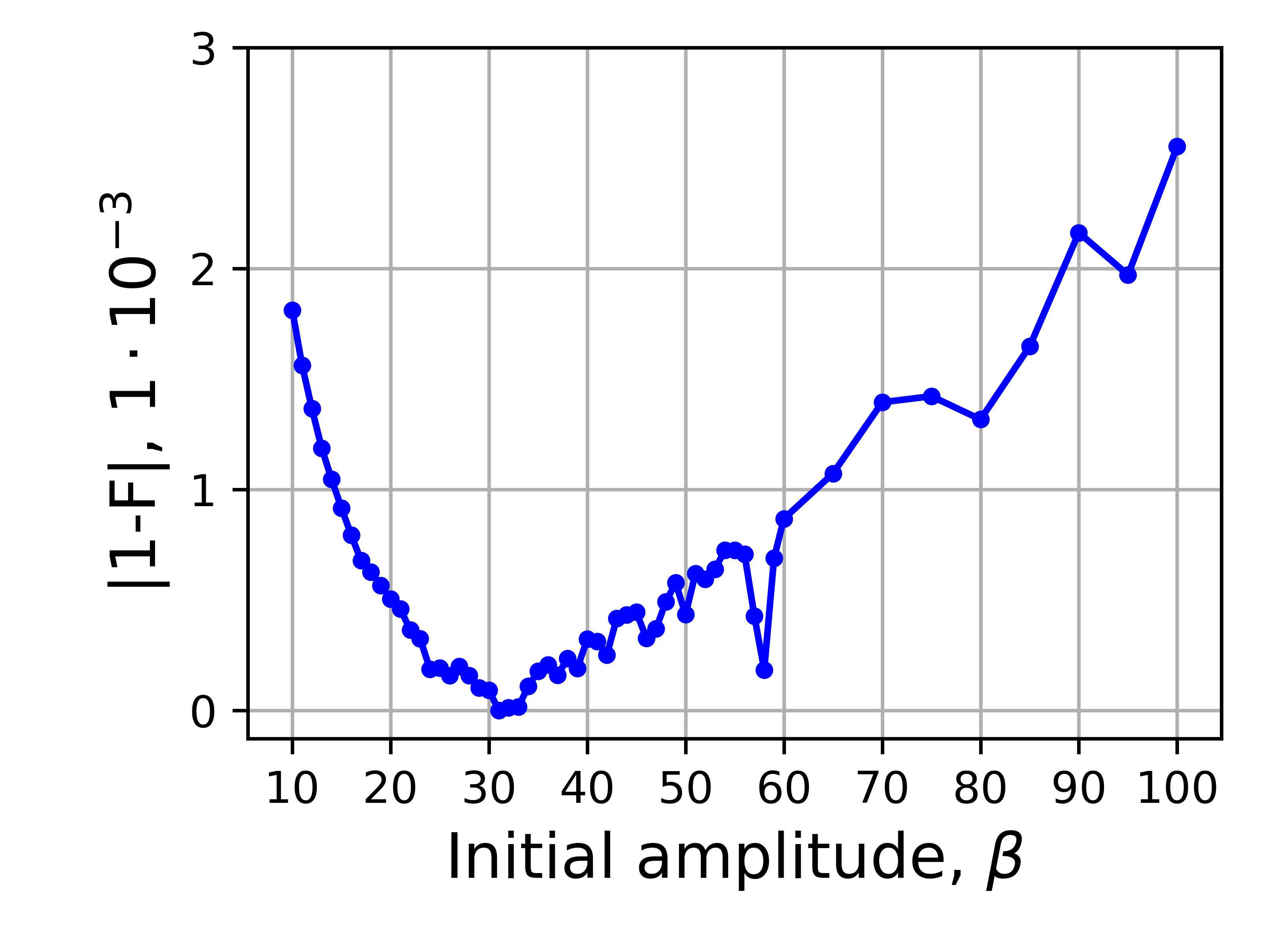
Figure 6: Deviation of the fidelity (16) from unity as a function of the amplitude in of the pump mode state $\beta$.

In Fig. 6, deviation of the resulting fidelity from one is plotted as a function of $\beta$. It does not exceed $3\times 10^{-3}$ and most probably results from the accumulated errors of the numerical calculations.

V Estimates

Consider the possibility of using the proposed method in optical whispering gallery mode resonators (WGMRs) that could have a large interaction coefficient $\gamma$ in the optical band [22, 23] due to high concentration of the optical energy in the small volumes of the optical modes.

In the case of isotropic medium and rectangular spatial distribution of the optical fields, the degenerate second-order non-linearity is described by the following Hamiltonian [24, 25]:

$$\hat{H}^{(2)}=-\frac{\epsilon_{0}\chi^{(2)}V}{2}E^{(+)}_{p}\Big{(}E^{(-)}_{s}\Big{)}^{2}+c.c.\,,$$ (18)

where $E^{(\pm)}_{p}$, $E^{(\pm)}_{s}$ are the rotating wave amplitudes of the electric field strengths of, respectively, the pump and signal modes. They can be quantized as follows:

$$\hat{E}^{(-)}_{s}=i\sqrt{\frac{\hbar\omega_{s}\nu_{s}}{2V\epsilon_{0}cn_{s}}}\hat{a}^{\dagger};\ \hat{E}^{(+)}_{p}=\sqrt{\frac{\hbar\omega_{p}\nu_{s}}{2V\epsilon_{0}cn_{p}}}\hat{b}\,,$$ (19)

where where $\nu_{s},\nu_{p}$ are the group velocity of the respective modes. Assuming for simplicity, that $\nu_{s,p}=c/n_{s,p}$ and substituting Eqs. (19) into (18), we recover the Hamiltonian (1) with

$$\gamma=\frac{\chi^{(2)}\omega_{s}}{4\sqrt{2}n_{s}^{2}n_{p}}\sqrt{\frac{\hbar\omega_{p}}{V\epsilon_{0}}}$$ (20)

With regard to the nonlinear media, the most suitable materials with the second order nonlinearity are either lithium niobate or lithium tantalate [26, 27]. Here we consider the lithium niobate.

We use the following values for our estimates:

$$\chi^{(2)}=2\times 10^{-11}\,\text{m/V}\,,$$

$$\omega_{s}=1.25\times 10^{15}\,\text{s}^{-1}\quad(\lambda_{s}=1.55\,\mu\text{m})\,,$$

$$\omega_{p}=2.5\times 10^{15}\,\text{s}^{-1}\quad(\lambda_{p}=775\,\text{nm})\,,$$

$$V=5.2\times 10^{-15}{\rm m^{3}}\,,$$

$$n_{s}=2.2111\,,\quad n_{p}=2.2587\,,$$

see [28, 29, 30]. Substituting them into Eq. (20), we obtain:

$$\gamma\approx 1\times 10^{7}\,\text{s}^{-1}\,.$$ (22)

It is well known that the non-Gaussian quantum states are readily destroyed by the optical losses. Therefore, implementation of the SC preparation procedure considered here requires that the optical losses in the WGMR have to be sufficiently small:

$$\varkappa\lesssim\gamma\,,$$ (23)

where $\varkappa$ is the bandwidth of the resonator. Taking into account the estimate (22) and assuming that $\lambda_{s}=1.55\,\mu\text{m}$, we obtain the following condition for the Q-factor of the WGMR:

$$Q=\frac{\omega_{s}}{\varkappa}\gtrsim 10^{8}\,.$$ (24)

This requirement is strict, but it can not be considered as an unrealistic one, see e.g. Ref. [29].