Positivity properties of scattering amplitudes
Abstract
We investigate positivity properties in quantum field theory (QFT). We find that planar Feynman integrals in QFT, as well as many related quantities, satisfy an infinite number of positivity conditions: the functions, as well as all their signed derivatives, are non-negative in a specified kinematic region. Such functions are known as completely monotonic (CM) in the mathematics literature. A powerful way to certify complete monotonicity is via integral representations. We thus show that it applies to non-planar integrals possessing a Euclidean region, to cosmological correlators, as well as to certain stringy integrals. Motivated by Positive Geometry, we investigate positivity properties in planar maximally supersymmetric Yang-Mills theory. We present evidence, based on known analytic multi-loop results, that the CM property extends to several physical quantities in this theory. This includes the (suitably normalized) finite remainder function of the six-particle maximally-helicity-violating (MHV) amplitude, four-point scattering amplitudes on the Coulomb branch, four-point correlation functions, as well as the angle-dependent cusp anomalous dimension. Our findings are however not limited to supersymmetric theories. It is shown that the CM property holds for the QCD and QED cusp anomalous dimensions, to three and four loops, respectively. We comment on open questions, and on possible numerical applications of complete monotonicity.
I Introduction
Positivity properties in QFT are often related to fundamental physical principles, such as unitarity and analyticity. Examples are bounds on effective field theory coefficients Arkani-Hamed et al. (2021a); Bellazzini et al. (2021), or the conformal bootstrap Simmons-Duffin (2017). The Positive Geometry program, initiated in ref. Arkani-Hamed and Trnka (2014); Hodges (2013), aims at a novel definition of quantum field theory. For scattering amplitudes, the starting point is a geometric object defined by the kinematic data of the scattered particles. The canonical form of this geometry corresponds to the scattering amplitudes (or, at loop level, to their integrand). This suggests a picture where the integrands can be thought of as volumes and are hence positive. It is an interesting question to explore if the integrated objects also have positivity properties. In this Letter we provide evidence in favor of this by reporting on a surprising infinite set of positivity constraints involving scattering amplitudes and their derivatives.
Let us briefly introduce the relevant mathematical concepts. A completely monotonic function in a region satisfies an infinite number of positivity conditions Widder (1941),
| (1) |
In other words, the function and all of its signed derivatives are positive. In particular, this means that such functions are non-negative, monotonically decreasing, and convex. This leads to typical shapes, cf. Figs. 1,2 for examples. It is remarkable that despite the rich analytic structure of the functions, their plots are rather featureless. The fact that such functions have ‘completely boring’ plots may be a virtue when it comes to numerical predictions in situation where full analytic results are not available, or that are time-intensive to evaluate numerically.
Let us quickly review useful features of CM functions. They are closed under multiplication and under taking convex sums: given two CM functions , and for , are again CM functions. Likewise, one may generate further CM functions by taking (signed) derivatives, or by integrating (with a suitable choice of boundary constant). Simple examples of CM functions are with and with are CM in , as can be verified by differentiation. The Bernstein-Haussdorff-Widder (BHW) theorem Widder (1941) states that a function is completely monotonic on if and only if it is the Laplace transform of a non-negative function , i.e.,
| (2) |
An example is
| (3) |
which is manifestly non-negative.
Note that the CM property depends on both the choice of variable and region. In general, composition of functions does not preserve it. However, if is completely monotonic and is absolutely monotonic (i.e., itself and all of its derivatives are non-negative), then is CM. Moreover, complete monotonicity is preserved under taking limits.
The multi-variable version of CM functions satisfies
| (4) |
by definition, and with a generalized version of the HBW theorem due to Choquet Choquet (1983). As a two-variable example, the following function appears in a finite seven-point one-loop integral Arkani-Hamed et al. (2011),
| (5) | ||||
It is useful to consider
| (6) |
which has the dispersive integral representation,
| (7) |
From this equation it is manifest that is CM on . Moreover, thanks to the product rule, and in view of eq. (6), we can deduce that is CM, as long as .
II Abundance of CM functions in QFT
We show that CM functions show up in numerous QFT building blocks. This is easily seen from suitable integral representations, as we explain presently.
The most important case is that of Feynman integrals. Consider the Feynman parametrization. In the latter, the Mandelstam variables and masses enter via a (negative) power of the so-called polynomial only, which in turn depends on them linearly. The kinematic domain in which is non-negative, if it exists, is called the Euclidean region. In the case the latter exists, scalar Feynman integrals are CM functions of the relevant combinations of Mandelstam variables and masses As an example, the one-loop massive bubble integral in two dimensions has the following Feynman representation,
| (8) |
where . It is a CM function of for , as can be seen by differentiating under the integral in eq. (8).
The Euclidean region exists for all planar integrals, and also for non-planar integrals for sufficiently general kinematics. For example, the four-point non-planar integrals considered in ref. Henn et al. (2014) have a Euclidean region if one external leg is off-shell, but not otherwise. A sufficient criterion for the existence of a Euclidean region was given in reference Mizera (2021).
We can use integral representations to ascertain the CM property for further relevant classes of quantum field theory objects. An example are the integral representations for cosmological correlators discussed in Arkani-Hamed et al. (2023). E.g.
| (9) | ||||
represents the contribution of a scalar tree-level diagram to the four-point wavefunction coefficient in a general Friedmann–Robertson–Walker (FRW) spacetime. We see that in eq. (9) is CM for .
Another example is the famous Veneziano formula,
| (10) |
One can see that this is CM in for by noticing that a derivative in (or ) inserts an extra factor of (or ) into the integrand, which is uniformly negative in the integration domain. This analysis can be extended to more general stringy canonical forms by virtue of the -representation, cf. section 9.4 of ref. Arkani-Hamed et al. (2021b),
| (11) |
Importantly, in this formula, , which makes it manifest that these integrals are CM in the interior of the Newton polytope defined by , which is where the integrals converge Berkesch et al. (2011). This is closely related to positivity certificates of Euler-type integrals discussed in reference Kozhasov et al. (2019).
Finally, there is a close connection between complete monotonicity and dispersion relations. For example, consider an unsubtracted dispersion relation,
| (12) |
where is the discontinuity of for . Using the Schwinger trick , this can be rewritten as eq. (2), with and
| (13) |
From eq. (12) we see that is a CM function of , provided that is non-negative. However, a weaker necessary condition is that in eq. (13) is non-negative. The above analysis can be generalized to Mandelstam representations Mandelstam (1959).
The above cases cover many building blocks in quantum field theory. However, physical quantities are usually linear combinations of those building blocks, with typically non-uniform signs, and additional kinematic factors that may change the sign properties of the functions, e.g. when taking derivatives. It is therefore interesting to ask: are there physical quantities that are completely monotone, as opposed to just their building blocks?
III Positivity of six-particle sYM amplitudes
An important motivation for expecting that this may be true comes from Positive Geometry. The prime example of a positive geometry is the Amplituhedron, which determines the loop integrands in planar super-Yang-Mills (sYM), which are rational functions. These integrands have a volume interpretation, and they are positive within the Amplituhedron region Hodges (2013); Arkani-Hamed et al. (2012a); Arkani-Hamed and Trnka (2014). What happens when one integrates the integrand over Minkowski space? The authors of Arkani-Hamed et al. (2015) found evidence that the finite part of integrated amplitudes is also positive, when evaluating the external kinematics within the tree Amplituhedron region.
The choice of infrared subtraction scheme presents a subtlety. For MHV amplitudes, the authors of Dixon et al. (2017) suggested to consider the ‘BDS-like-subtracted remainder function’ . Let us discuss this case in detail. The six-particle tree MHV Amplituhedron region is
| (14) | ||||
We expand quantities in planar sYM perturbatively in the Yang-Mills coupling using the following notation (and likewise for other quantities considered below),
| (15) |
where . The authors of reference Dixon et al. (2017) found that for , , for kinematics in . They showed this analytically in certain limits and on kinematic slices, and by numerical evaluation for randomly chosen kinematic points in . They also found evidence of monotonicity in a double scaling limit.
In this paper, we provide evidence that is CM in . We prove this analytically for , and provide numerical evidence at .
We begin by proving complete monotonicity at one loop. We have Dixon et al. (2017)
| (16) |
with
| (17) |
Note that implies . Therefore it is sufficient to prove that is CM for . We first note that . Therefore, if we can prove that is CM, then the same property for follows via integration. To this end, we compute
| (18) |
The RHS of this equation is a product of CM functions, and is hence CM itself, which completes the proof.
At two loops, is given by a weight four function Goncharov et al. (2010); Dixon et al. (2017). We outline the proof that this function is CM below. We employ a representation derived in Dixon et al. (2012), namely
| (19) | ||||
Here is a finite double pentagon integral Arkani-Hamed et al. (2012b); Dixon et al. (2012), and is a weight-four function, expressed in terms of harmonic polylogarithms Gehrmann and Remiddi (2001). We prove that is CM for by differentiation, and employing a dispersive representation. Next, we use Dixon et al. (2012),
| (20) |
where is a finite penta-box integral Drummond et al. (2011). The latter is seen to be CM for by considering its Feynman parametrization, in agreement with the CM property discussed above for its one-loop version . Finally, is a scalar hexagon integral, which is CM, and hence so is . This completes the proof.
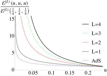
At three and four loops, we performed the following numerical checks of complete monotonicity. Employing the analytic formulas computed in refs. Dixon et al. (2013, 2014); Dixon , we evaluated both and all of its first two derivatives numerically for phase-space points within . We used Bauer et al. (2002); Duhr and Dulat (2019) for the numerical evaluation. Fig. 1 shows an interpolated plot for , for which becomes . The AdS curve corresponds to the strong coupling result Alday et al. (2011); Basso et al. (2014, 2020), , with 111We thank Lance Dixon for insightful correspondence regarding the constants in eq. (21).
| (21) |
Note that is CM for .
IV Evidence of complete monotonicity of further physical quantities
We present evidence of the CM property for several further quantities in planar sYM. In the first three cases, this evidence is based on numerical evaluation of the functions and their first two derivatives, as well as on numerical evaluation (whenever feasible) of the inverse Laplace transform. In the fourth case, the CM property can be proven.
1. Four-point Coulomb branch amplitudes Alday et al. (2010), which depend on the kinematic variables . We find numerical evidence that is a CM function of , for using the available results Caron-Huot and Henn (2014) at . Let us recall the small mass limit Alday et al. (2010); Brüser et al. (2018), in which
| (22) |
where is the light-like cusp anomalous dimension Beisert et al. (2007). We see that eq. (22) is consistent with the CM property as follows: First, the argument of the exponential is CM because and are CM functions for argument smaller than one, and because . Second, the exponential of a CM function is also a CM function.
2. Four-point deformed Amplituhedron amplitudes, computed to two loops in Arkani-Hamed et al. (2024). We find that are CM functions of , for , and .
3. Four-point correlation functions We find numerical evidence for given in eq. (1.1) of Drummond et al. (2013) being CM as functions of the cross-ratios given in eq. (1.11) of that paper, for (initially computed in Eden et al. (2000); Bianchi et al. (2000)). We leave the case for future work.
4. The angle-dependent cusp anomalous dimension, up to four loops, cf. eq. (5.3) of Henn and Huber (2013). We express it in terms of , which is related to the cusp angle by . We have, for example,
| (23) |
The RHS of eq. (23) is a CM function of . This follows from the fact that both factors are CM . Similarly, we were able to prove recursively that is a CM function of .
We note that is closely related to the logarithm of the Coulomb branch amplitudes discussed under 1., as the latter contain the cusp anomalous dimension in a Regge limit Henn et al. (2010), where , in which the variables are matched according to . This raises several important questions: is it more natural to look for CM properties of , or of , and in what variables? We leave these interesting questions, which are relevant to other quantities as well, to future investigations.
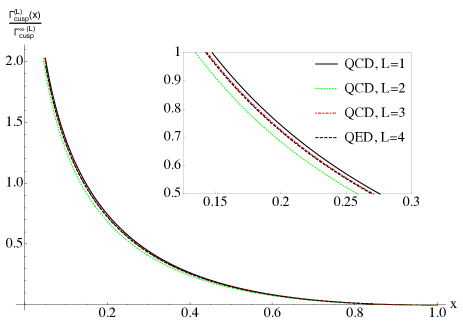
The above examples were from planar sYM. The CM property is however not limited to quantities in this theory. We found it also in the three-loop angle-dependent cusp anomalous dimension in QCD Grozin et al. (2015), and in the four-loop QED one Brüser et al. (2021). A comment is due regarding their numerical values. In the Euclidean region , they diverge logarithmically at zero, , while they vanish by definition at . Interestingly, as already noted in references Grozin et al. (2015); Brüser et al. (2021) (see also Kidonakis (2016)), if one normalizes the functions so that they have the same small asymptotics, their graphs are extremely similar, as shown in Fig. 2. (However, numerically, they differ by several per cent.) The remarkable similarity of the plots in that Figure suggests to us that complete monotonicity, together with physical input, could be useful for numerically approximating .
V Summary and Outlook
In this Letter, we have presented evidence that completely monotonic functions play an important role in scattering amplitudes, and in other quantities in QFT. In some cases complete monotonicity has an elementary explanation, such as integral representations, from which the infinite number of positivity properties are manifest. In other cases complete monotonicity is motivated by Positive Geometry, but remains to be proven.
Our findings open up several research directions:
1. Developing mathematical proofs for special functions from QFT. A pressing issue is to systematically develop methods for proving or disproving the CM property, for the relevant cases of special functions that appear in QFT. This would allow us to go from numerical evidence to rigorous statements about the CM property.
2. Exploring mathematical data to find out in which cases complete monotonicity holds. We are in the fortunate situation to have access to a wealth of analytically known scattering amplitudes, such as for example at higher loops Dixon and Liu (2023), for amplitudes with helicity configurations beyond MHV Arkani-Hamed et al. (2015), for higher-point Wilson loops with Lagrangian insertions Chicherin and Henn (2022), as well as for various QCD scattering amplitudes. It is exciting to study which of these functions have hidden CM properties.
3. Relating complete monotonicity to Positive Geometry. We find it likely that the connection to Positive Geometry could lead to a proof of the CM property for suitable quantities (and, along the way, inform us about a choice of natural variables in which to find the CM property). For example, for convex polytopes one can write the canonical rational function at any interior point as a Laplace transform on the dual cone Arkani-Hamed et al. (2017),
| (24) |
This suggests to us a close connection between the CM property and dual geometries. This could help when looking for a dual geometry in cases beyond polytopes, such as the conjectured dual Amplituhedron Arkani-Hamed et al. (2012a); Ferro et al. (2016); Herrmann et al. (2021).
4. Exploring connections to analyticity and unitarity. Another promising direction is to investigate the relation of the CM property to physically expected properties of the S-matrix Eden et al. (1966); Correia et al. (2021). For example, it would be fascinating to explore in which contexts the CM property can be derived from dispersion relations, e.g. by using positivity properties of the imaginary part of the amplitudes, cf. e.g. Jin and Martin (1964); Martin (1965) and eq. (13). We note that there are interesting related findings of notions of positivity in the context of renormalization group flow Hartman and Mathys (2024), and for forward amplitudes Hui et al. (2024).
5. Harnessing implications of complete monotonicity. The combination of positivity and convexity has proven to be a successful recipe in physics. This is well appreciated in the context of the conformal field theory and S-matrix bootstrap programs Simmons-Duffin (2017); Kruczenski et al. (2022), where these principles are used to constrain the space of allowed theories. We expect that the knowledge of an infinite number of positivity constraints and convexity of the space of CM functions may be useful for numerical approximations or bootstrap approaches. Just to give one example, the additional information we provide may be used to improve the method proposed in Zeng (2023) for numerically bootstrapping Feynman integrals. Another direction is to combine positivity with recent machine learning approaches to the symbol bootstrap Cai et al. (2024). Finally, it would be interesting to explore implications for analytically continued kinematic regions, which are relevant to phenomenological applications of scattering amplitudes. We expect the concept of positive real functions Seshu and Seshu (1961) to be useful in this regard.
Acknowledgments
It is a pleasure to thank Nima Arkani-Hamed, Lance Dixon, Yifei He, Martín Lagares, Elia Mazzucchelli, Sebastian Mizera, Alessandro Podo, Giulio Salvatori, Bernd Sturmfels, and Jaroslav Trnka for discussions. We also thank Jungwon Lim and Chenyu Wang for help with numerical computations, and Yang Zhang for correspondence. Funded by the European Union (ERC, UNIVERSE PLUS, 101118787). Views and opinions expressed are however those of the authors only and do not necessarily reflect those of the European Union or the European Research Council Executive Agency. Neither the European Union nor the granting authority can be held responsible for them.
References
- Arkani-Hamed et al. (2021a) N. Arkani-Hamed, T.-C. Huang, and Y.-t. Huang, JHEP 05, 259 (2021a), arXiv:2012.15849 [hep-th] .
- Bellazzini et al. (2021) B. Bellazzini, J. Elias Miró, R. Rattazzi, M. Riembau, and F. Riva, Phys. Rev. D 104, 036006 (2021), arXiv:2011.00037 [hep-th] .
- Simmons-Duffin (2017) D. Simmons-Duffin, in Theoretical Advanced Study Institute in Elementary Particle Physics: New Frontiers in Fields and Strings (2017) pp. 1–74, arXiv:1602.07982 [hep-th] .
- Arkani-Hamed and Trnka (2014) N. Arkani-Hamed and J. Trnka, JHEP 10, 030 (2014), arXiv:1312.2007 [hep-th] .
- Hodges (2013) A. Hodges, JHEP 05, 135 (2013), arXiv:0905.1473 [hep-th] .
- Widder (1941) D. Widder, The Laplace Transform, Princeton mathematical series (Princeton University Press, 1941).
- Choquet (1983) G. Choquet, in Measure Theory and its Applications, edited by J.-M. Belley, J. Dubois, and P. Morales (Springer Berlin Heidelberg, Berlin, Heidelberg, 1983) pp. 114–125.
- Arkani-Hamed et al. (2011) N. Arkani-Hamed, J. L. Bourjaily, F. Cachazo, S. Caron-Huot, and J. Trnka, JHEP 01, 041 (2011), arXiv:1008.2958 [hep-th] .
- Henn et al. (2014) J. M. Henn, A. V. Smirnov, and V. A. Smirnov, JHEP 03, 088 (2014), arXiv:1312.2588 [hep-th] .
- Mizera (2021) S. Mizera, Phys. Rev. D 103, 081701 (2021), arXiv:2101.08266 [hep-th] .
- Arkani-Hamed et al. (2023) N. Arkani-Hamed, D. Baumann, A. Hillman, A. Joyce, H. Lee, and G. L. Pimentel, (2023), arXiv:2312.05303 [hep-th] .
- Arkani-Hamed et al. (2021b) N. Arkani-Hamed, S. He, and T. Lam, JHEP 02, 069 (2021b), arXiv:1912.08707 [hep-th] .
- Berkesch et al. (2011) C. Berkesch, J. Forsgrard, and M. Passare, arXiv e-prints , arXiv:1103.6273 (2011), arXiv:1103.6273 [math.CV] .
- Kozhasov et al. (2019) K. Kozhasov, M. Michałek, and B. Sturmfels, “Positivity certificates via integral representations,” (2019), arXiv:1908.04191 .
- Mandelstam (1959) S. Mandelstam, Phys. Rev. 115, 1741 (1959).
- Arkani-Hamed et al. (2012a) N. Arkani-Hamed, J. L. Bourjaily, F. Cachazo, A. Hodges, and J. Trnka, JHEP 04, 081 (2012a), arXiv:1012.6030 [hep-th] .
- Arkani-Hamed et al. (2015) N. Arkani-Hamed, A. Hodges, and J. Trnka, JHEP 08, 030 (2015), arXiv:1412.8478 [hep-th] .
- Dixon et al. (2017) L. J. Dixon, M. von Hippel, A. J. McLeod, and J. Trnka, JHEP 02, 112 (2017), arXiv:1611.08325 [hep-th] .
- Goncharov et al. (2010) A. B. Goncharov, M. Spradlin, C. Vergu, and A. Volovich, Phys. Rev. Lett. 105, 151605 (2010), arXiv:1006.5703 [hep-th] .
- Dixon et al. (2012) L. J. Dixon, J. M. Drummond, and J. M. Henn, JHEP 01, 024 (2012), arXiv:1111.1704 [hep-th] .
- Arkani-Hamed et al. (2012b) N. Arkani-Hamed, J. L. Bourjaily, F. Cachazo, and J. Trnka, JHEP 06, 125 (2012b), arXiv:1012.6032 [hep-th] .
- Gehrmann and Remiddi (2001) T. Gehrmann and E. Remiddi, Comput. Phys. Commun. 141, 296 (2001), arXiv:hep-ph/0107173 .
- Drummond et al. (2011) J. M. Drummond, J. M. Henn, and J. Trnka, JHEP 04, 083 (2011), arXiv:1010.3679 [hep-th] .
- Caron-Huot et al. (2016) S. Caron-Huot, L. J. Dixon, A. McLeod, and M. von Hippel, Phys. Rev. Lett. 117, 241601 (2016), arXiv:1609.00669 [hep-th] .
- Dixon et al. (2013) L. J. Dixon, J. M. Drummond, M. von Hippel, and J. Pennington, JHEP 12, 049 (2013), arXiv:1308.2276 [hep-th] .
- Dixon et al. (2014) L. J. Dixon, J. M. Drummond, C. Duhr, and J. Pennington, JHEP 06, 116 (2014), arXiv:1402.3300 [hep-th] .
- (27) L. J. Dixon, www.slac.stanford.edu/lance/R64/, Accessed: 2024-06-01.
- Bauer et al. (2002) C. W. Bauer, A. Frink, and R. Kreckel, J. Symb. Comput. 33, 1 (2002), arXiv:cs/0004015 .
- Duhr and Dulat (2019) C. Duhr and F. Dulat, JHEP 08, 135 (2019), arXiv:1904.07279 [hep-th] .
- Alday et al. (2011) L. F. Alday, D. Gaiotto, and J. Maldacena, JHEP 09, 032 (2011), arXiv:0911.4708 [hep-th] .
- Basso et al. (2014) B. Basso, A. Sever, and P. Vieira, Phys. Rev. Lett. 113, 261604 (2014), arXiv:1405.6350 [hep-th] .
- Basso et al. (2020) B. Basso, L. J. Dixon, and G. Papathanasiou, Phys. Rev. Lett. 124, 161603 (2020), arXiv:2001.05460 [hep-th] .
- Note (1) We thank Lance Dixon for insightful correspondence regarding the constants in eq. (21).
- Alday et al. (2010) L. F. Alday, J. M. Henn, J. Plefka, and T. Schuster, JHEP 01, 077 (2010), arXiv:0908.0684 [hep-th] .
- Caron-Huot and Henn (2014) S. Caron-Huot and J. M. Henn, JHEP 06, 114 (2014), arXiv:1404.2922 [hep-th] .
- Brüser et al. (2018) R. Brüser, S. Caron-Huot, and J. M. Henn, JHEP 04, 047 (2018), arXiv:1802.02524 [hep-th] .
- Beisert et al. (2007) N. Beisert, B. Eden, and M. Staudacher, J. Stat. Mech. 0701, P01021 (2007), arXiv:hep-th/0610251 .
- Arkani-Hamed et al. (2024) N. Arkani-Hamed, W. Flieger, J. M. Henn, A. Schreiber, and J. Trnka, Phys. Rev. Lett. 132, 211601 (2024), arXiv:2311.10814 [hep-th] .
- Drummond et al. (2013) J. Drummond, C. Duhr, B. Eden, P. Heslop, J. Pennington, and V. A. Smirnov, JHEP 08, 133 (2013), arXiv:1303.6909 [hep-th] .
- Eden et al. (2000) B. Eden, C. Schubert, and E. Sokatchev, Phys. Lett. B 482, 309 (2000), arXiv:hep-th/0003096 .
- Bianchi et al. (2000) M. Bianchi, S. Kovacs, G. Rossi, and Y. S. Stanev, Nucl. Phys. B 584, 216 (2000), arXiv:hep-th/0003203 .
- Henn and Huber (2013) J. M. Henn and T. Huber, JHEP 09, 147 (2013), arXiv:1304.6418 [hep-th] .
- Henn et al. (2010) J. M. Henn, S. G. Naculich, H. J. Schnitzer, and M. Spradlin, JHEP 04, 038 (2010), arXiv:1001.1358 [hep-th] .
- Grozin et al. (2015) A. Grozin, J. M. Henn, G. P. Korchemsky, and P. Marquard, Phys. Rev. Lett. 114, 062006 (2015), arXiv:1409.0023 [hep-ph] .
- Brüser et al. (2021) R. Brüser, C. Dlapa, J. M. Henn, and K. Yan, Phys. Rev. Lett. 126, 021601 (2021), arXiv:2007.04851 [hep-th] .
- Kidonakis (2016) N. Kidonakis, Int. J. Mod. Phys. A 31, 1650076 (2016), arXiv:1601.01666 [hep-ph] .
- Dixon and Liu (2023) L. J. Dixon and Y.-T. Liu, JHEP 09, 098 (2023), arXiv:2308.08199 [hep-th] .
- Chicherin and Henn (2022) D. Chicherin and J. M. Henn, JHEP 07, 057 (2022), arXiv:2202.05596 [hep-th] .
- Arkani-Hamed et al. (2017) N. Arkani-Hamed, Y. Bai, and T. Lam, JHEP 11, 039 (2017), arXiv:1703.04541 [hep-th] .
- Ferro et al. (2016) L. Ferro, T. Lukowski, A. Orta, and M. Parisi, JHEP 03, 014 (2016), arXiv:1512.04954 [hep-th] .
- Herrmann et al. (2021) E. Herrmann, C. Langer, J. Trnka, and M. Zheng, JHEP 01, 035 (2021), arXiv:2009.05607 [hep-th] .
- Eden et al. (1966) R. J. Eden, P. V. Landshoff, D. I. Olive, and J. C. Polkinghorne, The analytic S-matrix (Cambridge Univ. Press, Cambridge, 1966).
- Correia et al. (2021) M. Correia, A. Sever, and A. Zhiboedov, JHEP 03, 013 (2021), arXiv:2006.08221 [hep-th] .
- Jin and Martin (1964) Y. S. Jin and A. Martin, Phys. Rev. 135, B1369 (1964).
- Martin (1965) A. Martin, Nuovo Cim. A 42, 930 (1965).
- Hartman and Mathys (2024) T. Hartman and G. Mathys, JHEP 01, 102 (2024), arXiv:2310.15217 [hep-th] .
- Hui et al. (2024) L. Hui, I. Kourkoulou, A. Nicolis, A. Podo, and S. Zhou, JHEP 04, 145 (2024), arXiv:2312.08440 [hep-th] .
- Kruczenski et al. (2022) M. Kruczenski, J. Penedones, and B. C. van Rees, (2022), arXiv:2203.02421 [hep-th] .
- Zeng (2023) M. Zeng, JHEP 09, 042 (2023), arXiv:2303.15624 [hep-ph] .
- Cai et al. (2024) T. Cai, G. W. Merz, F. Charton, N. Nolte, M. Wilhelm, K. Cranmer, and L. J. Dixon, (2024), arXiv:2405.06107 [cs.LG] .
- Seshu and Seshu (1961) S. Seshu and L. Seshu, Journal of Mathematical Analysis and Applications 3(3), 592 (1961).