Dark Sector Tunneling Field Potentials for a Dark Big Bang

Abstract

All of the significant evidence for dark matter observed thus far has been through its gravitational interactions. After 40 years of direct detection experiments, the parameter space for Weakly Interacting Massive Particles (WIMPs) as dark matter candidates is rapidly approaching the neutrino floor. In this light, we consider a dark sector that is strongly decoupled from the visible sector, interacting exclusively through gravity. In this model, proposed by Freese and Winkler [1], dark matter can be produced through a first-order phase transition in the dark sector dubbed “The Dark Big Bang”. In this study, we fully determine the allowed region of parameter space for the tunneling potential that leads to the realization of a Dark Big Bang and is consistent with all experimental bounds available.

I Introduction

Dark matter has been researched since the 1930s and the fact that it exists in the universe is well established. The early indicators of dark matter’s existence came from extragalactic data. To explain the velocities of galaxies within clusters [2] and the internal stability of galaxies themselves requires the presence of extra non-luminous mass [3, 4, 5]. Advanced measurements of the anisotropies in the Cosmic Microwave Background (CMB) have provided the strongest evidence for the existence of dark matter. In 2018, the Planck collaboration found that 27% of the energy of the universe is in dark matter, while only 5% is in Standard Model (SM) particles [6]. The interested reader can refer to this comprehensive history of the discovery and ongoing search for dark matter [7]. Modern research efforts aim to uncover the properties of dark matter particles through particle colliders [8], direct detection experiments [9], and observations of the universe [10, 11, 12].

WIMPs have been the leading candidate for particle dark matter since these are the lightest particles arising from a supersymmetric extension to the standard model. Supersymmetry is a theoretical model proposing the existence of an array of yet-undetected particles mirroring the standard model. Supersymmetry helps explain the mass value of the Higgs boson and the vacuum energy of the universe. Since WIMPs are the lightest of these particles, they should be the most easily detected. Yet besides a contentious signal from the DAMA collaboration (which may be verified or ruled-out in upcoming direct detection experiments such as COSINE-100 [13]), no WIMPs have been conclusively detected. In fact, the parameter space above the neutrino floor is almost ruled out entirely (see [14]). In this light, two of the possible paths for dark matter research are to come up with direct detection experiments below the neutrino floor [15] or to abandoned the weakly-interacting model entirely. This work will focus on the latter path.

Strongly decoupled dark matter only interacts with the visible sector through gravity. This is known as the “nightmare scenario” for physicists looking for dark matter. Gravity is by far the weakest of the fundamental forces in nature, so if this is the only way dark matter speaks to the visible universe, it will be very hard to detect. The Dark Big Bang theory, proposed in 2023 by Freese and Winkler [1], makes the nightmare a little less scary. If dark matter originated in a Dark Big Bang (DBB), gravity waves produced in the phase transition could be detected, providing a source of evidence for this decoupled dark matter [1].

The Dark Big Bang model proposes that dark and visible matter could have different origins in the early universe, assuming that dark matter is strongly decoupled from the visible sector. Initially, the dark sector is cold and has energy density $\rho_{\phi}$, which is always subdominant to the energy density of the visible sector [1]. Eventually, the dark false vacuum will decay, analogous to the vacuum decay of the standard Hot Big Bang scenario. The dark sector then goes through a period of reheating, producing a dark sector thermal bath denoted by $T_{\rm{DS}}$. The DBB model has been shown to successfully produce a wide range of dark matter particles with masses $\mathcal{O}$(keV - 10¹²GeV) [1] making it a versatile origin for many different dark matter particle models. In fact, a DBB could be possible with a dark sector that interacts weakly with the visible sector through portals such as the Higgs, neutrino, vector, or axion portal. These DBB scenarios have yet to be researched.

The theory of the Dark Big Bang is constrained to be consistent with standard $\Lambda$CDM cosmology and cosmological observations. The purpose of this paper is to impose these constraints onto the initial conditions of the DBB, explicitly determining the parameter space of the dark sector tunneling field potential which governs many aspects of the phase transition. We will show the parameter space for the tunneling field potential has two distinct regions. Parameters from one of the regions have not yet been utilized for a benchmark DBB, so this region will be of specific interest. We will show that a DBB with parameters chosen from this new region can produce the correct relic abundance of dark matter in the universe.

II A Phase Transition in the Dark Sector

II.1 Background

The Dark Big Bang occurs through a first-order phase transition in the dark sector. Since the dark sector is initially cold, the phase transition occurs through the quantum tunneling of the $\phi$ field through a potential barrier (as opposed to thermal fluctuations causing $\phi$ to jump over the potential barrier). Initially, all of the dark sector energy density resides in the tunneling field $\phi$. This phase transition can be modeled like a particle in a potential with two non-degenerate minima. An illustrative example is shown in Fig.1[1].

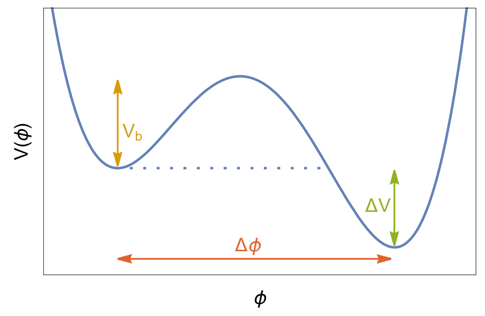
Figure 1: Model tunneling field potential used for a first-order phase transition in the dark sector [1]. At the beginning of the universe, $\phi$ sits in the metastable minimum of the potential well. The discontinuous phase transition is realized when $\phi$ quantum tunnels through the potential barrier and eventually comes to rest in the ultrastable minimum. The height of the potential barrier is denoted by $V_{\rm{b}}$. The separation between the two minima is $\Delta\phi$. The change in potential of $\phi$ through the phase transition is $\Delta V$.

While the dark sector is in the false vacuum state ($\phi$ sits in the metastable minimum of $V(\phi)$), quantum fluctuations cause bubbles of the true vacuum to randomly nucleate throughout the universe. If the bubbles nucleate with a large enough radius, expansion will be energetically favored over collapse and the bubbles will expand and collide [16]. In Fig. 1, this can be modelled by the $\phi$ field quantum tunneling through the potential barrier and materializing at a height $V(\phi)=\Delta V$ near the ultrastable minimum with zero kinetic energy. As $\phi$ rolls towards the ultrastable minimum, the kinetic energy gained is stored in the expanding bubble walls [16]. $\phi$ will then undergo oscillations around the ultrastable minimum, which are dampened by couplings to dark sector fields. As $\phi$ comes to a rest in the true vacuum state, bubble walls collide, releasing their energy into dark sector fields and gravity waves. A first-order phase transition is phenomenologically similar to the phase transition of super-heated water to gas [16]: bubbles of the new phase (gas) nucleate and expand in the old phase (water) until all of the water has been turned into gas.

The Lagrangian for the dark sector is [1]

$$\mathcal{L}_{\rm{DS}}=\frac{1}{2}\partial_{\mu}\phi\partial^{\mu}\phi+\frac{1}{2}\partial_{\mu}\chi\partial^{\mu}\chi-V(\phi)-y\phi^{2}\chi^{2}-\frac{m_{\chi}^{2}}{2}\chi^{2}-\kappa\chi^{4}\hskip 5.69054pt(+\mathcal{L}_{\rm{DR}})$$ (1)

where both $\phi$ and $\chi$ are taken to be real scalars, and $\mathcal{L}_{\rm{DR}}$ is the dark radiation Lagrangian density, if dark radiation is included in the model being considered. The tunneling field potential $V(\phi)$ takes the form [1]

$$V(\phi)=\frac{m^{2}}{2}\phi^{2}-\mu\phi^{3}+\lambda\phi^{4}+\Delta V$$ (2)

to allow for two non-degenerate potential minima. Placing the metastable minimum at $\phi=0$ requires $\mu>\sqrt{2\lambda}m$, where $m$ is the mass of of the tunneling field in the false vacuum state and $\mu$, $\lambda$ govern $\phi$ interactions. The true minimum of $V(\phi)$ is then [1]

$$\phi_{min}=\frac{3\mu+\sqrt{9\mu^{2}-16\lambda m^{2}}}{8\lambda}=\Delta\phi$$ (3)

which is found by setting $V^{\prime}(\phi)=0$ and taking the positive root. Since $\Delta V=V(0)-V(\phi_{\rm{min}})$, $\Delta V$ can be solved for algebraically [1]

$$\Delta V=\frac{(3\mu+\sqrt{9\mu^{2}-16\lambda m^{2}})^{2}}{64\lambda^{2}}\left(\frac{3\mu^{2}+\mu\sqrt{9\mu^{2}-16\lambda m^{2}}-8\lambda m^{2}}{32\lambda}\right)$$ (4)

Using a similar approach, the barrier height is

$$V_{b}=\frac{(3\mu-\sqrt{9\mu^{2}-16\lambda m^{2}})^{2}}{64\lambda^{2}}\left(\frac{-3\mu^{2}+\mu\sqrt{9\mu^{2}-16\lambda m^{2}}+8\lambda m^{2}}{32\lambda}\right)$$ (5)

The $\phi$ field undergoes a mass shift during the phase transition. When $\phi$ is in the true vacuum state, its mass becomes [1]

$$m_{\phi}^{2}=V^{\prime\prime}(\Delta\phi)=\frac{9\mu^{2}+3\mu\sqrt{9\mu^{2}-16\lambda m^{2}}}{8\lambda}-2m^{2}$$ (6)

which can be seen through the MacLaurin Series expansion of $V(\phi)$ around the metastable minimum.

II.2 Phase Transition Parameters

Many of the physical characteristics of a DBB are determined by the shape and scale of the tunneling potential $V(\phi)$. This paper will focus on the two parameters that are constrained by cosmological observations: the visible sector temperature at the time of the DBB ($T_{*}$) and the strength of the DBB ($\alpha$). The strength of the DBB is defined as the ratio of dark to visible sector energy densities directly after the phase transition [1]. Since the DBB occurs early in the universe during the radiation-dominated epoch, the total energy density of the visible sector can be approximated as the energy stored in radiation. The strength of the DBB can be written as [1]

$$\alpha\simeq\frac{\rho_{\phi}}{\rho_{r,*}}\simeq\frac{\Delta V}{\frac{\pi^{2}}{30}g_{\rm{eff}}(T_{*})T_{*}^{4}}$$ (7)

The _∗ subscript notation means the variable is evaluated at the time of the DBB. We have also defined the energy density of the dark sector before the phase transition as $\rho_{\rm{DS}}\simeq\rho_{\phi}=\Delta V$ [1]. The DBB theory accounts for the creation of all dark matter in the decay of the dark false vacuum, so dark matter particles must be produced efficiently in this phase transition. This requires the presence of light degrees of freedom in the dark sector $g_{\rm{DS}}$ that the bubble walls can always efficiently decay into [1]. With these light degrees of freedom in the dark sector, the end of the phase transition is considered a period of dark sector reheating, and the dark plasma produced quickly reaches a thermal equilibrium described by $T_{\rm{DS}}$ [1]. Gravity waves make up at most 5% of the dark sector energy density released in the phase transition [1], so the energy density in the dark sector after the phase transition can be approximated by [1]

$$\rho_{\phi}=\Delta V\simeq\frac{\pi^{2}}{30}g_{\rm{DS}}(T_{\rm{DS}})T_{\rm{DS}}^{4}$$ (8)

With this approximation, the dark reheating temperature can then be defined as [1]

$$T_{\rm{DS,*}}\simeq\left(\frac{30}{\pi^{2}g_{\rm{DS,*}}}\Delta V\right)^{1/4}$$ (9)

where $g_{\rm{DS,*}}\equiv g_{\rm{DS}}(T_{\rm{DS,*}})$. Then $\alpha$ is the ratio of the dark sector reheating temperature to the visible sector temperature when the DBB occurs, up to their respective degrees of freedom

$$\alpha\approx\frac{g_{\rm{DS},*}}{g_{\rm{eff},*}}\left(\frac{T_{\rm{DS},*}}{T_{*}}\right)^{4}$$ (10)

II.3 Bounds From the Early Universe

The DBB is bounded to be consistent with cosmological observations and standard $\Lambda$CDM cosmology. The bounds are discussed at length in Ref. [1] and we will provide a brief overview here. The lower limit on $\alpha$ is determined by the requirement that the energy released in the phase transition can account for all dark matter in the universe today [1]. In mapping the power spectrum of CMB anisotropies, the Planck collaboration determined today’s dark matter density to be $\rho_{\rm{DM},0}=1.26$ keVcm^-3  [6]. Using the scale factor at the time of the DBB $a_{*}$ to translate this to be a constrain on $\alpha$, the lower bound on the strength of the DBB becomes [1]

$$\alpha\geq\frac{\rho_{\rm{DM},0}}{a_{*}^{3}\rho_{r,*}}=\frac{4}{3}\frac{\rho_{\rm{DM},0}}{s_{0}T_{*}}=5.8\times 10^{-7}\left(\frac{\rm{MeV}}{T_{*}}\right)$$ (11)

where radiation density has been put in terms of entropy density of the visible sector $\rho_{r,*}=(3/4)s_{*}T_{*}$ and conservation of entropy $s_{*}a_{*}^{3}=s_{0}$ has been utilized.

The upper limit of $\alpha$ comes from existing bounds on the amount of extra energy density present in the early universe (in the DBB scenario, that extra energy density is $\rho_{\rm{DS}}$) [1]. Extra energy density causes a speed up of the expansion of the universe realized as an increase in the Hubble parameter $H$. The speed up could cause weak interactions to freeze out earlier in the universe leading to an increase in the relativistic species populating the early universe $N_{\rm{eff}}$. $N_{\rm{eff}}$ counts the number of these relativistic species (not including photons), and is called the effective number of neutrinos (although particles other than neutrinos can contribute to $N_{\rm{eff}}$) [17]. An increase in this number leads to dampening in the small scale (large $\ell$) power spectrum of CMB anisotropies. The Standard Model predicts $N_{\rm{eff}}=3.046$ [17] and the Planck collaboration has determined bounds on the change in this number $\Delta N_{\rm{eff}}=0.22\pm 0.15$ [6]. Taking the weaker bound $\Delta N_{\rm{eff}}<0.5$ leads to the following upper limit on $\alpha$ [1]

$$\alpha<\left(\frac{2\pi^{2}}{45}\right)^{1/3}\frac{4g_{\rm{eff}}^{1/3}(T_{*})\rho_{\rm{DR},0}}{3s_{0}^{4/3}}<0.079\left(\frac{g_{\rm{eff}}(T_{*})}{10}\right)^{1/3}$$ (12)

where $\rho_{\rm{DR,0}}$ is the present dark radiation density $\rho_{\rm{DR,0}}\lesssim 29.6$ meVcm^-3 [1].

The final constraint is on the latest a DBB can occur to be consistent with the $\Lambda$CDM picture of structure formation. Requiring that dark matter obtains the correct adiabatic perturbations to seed structure formation leads to the strongest constraint on the latest a DBB can occur [1]. $\rho_{\phi}$ is a smooth fluid at the time of the DBB, so the dark matter content must pick up perturbations from the visible sector radiation bath which dominates the universe [1]. The radiation bath exhibits adiabatic perturbations, which are realized in a common, local time shift of all background quantities in cosmological perturbation theory [17]. Adiabatic perturbations are defined by the equality $\delta\rho_{r}(\eta,\textbf{x})=\bar{\rho_{r}}^{\prime}\pi(\eta,\textbf{x})$ where $\eta$ is conformal time and x is a three dimensional space coordinate. This equation says that perturbed quantities at some spacetime point are the same as those in the background universe at a slightly shifted spacetime point. Adiabatic perturbations in visible sector radiation cause the DBB phase transition to occur at slightly different times throughout the universe. These time differences result in the perturbations becoming imprinted on the dark matter produced in the DBB (see [1]).

Observations of Ly-$\alpha$ from distant quasars can be used to constrain these perturbations on large scales. Using existing constraints on cosmological fluctuations from warm dark matter simulations [18, 19], the approximate bound on the latest a DBB can occur is [1]

$$T_{*}>6.8\times 10^{-4}\rm{MeV}$$ (13)

The bounds on a DBB are shown in Fig. 2, which has been expanded from [1] to include higher temperatures. The main focus of our work is to map this parameter space onto the parameters determining the tunneling field potential. In the next section, we will show how the phase transition parameters can be recast as functions of the tunneling field parameters.

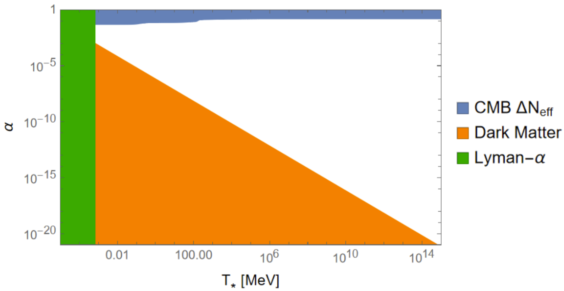
Figure 2: Bounds on the strength of a DBB and the latest a DBB can occur [1]. The allowed region for a DBB consistent with observations is the white space in the figure. The upper bound on $\alpha$ depends on the relativistic degrees of freedom in the universe and remains constant above the mass scale of the heaviest SM particle: top quarks m${}_{t}\sim 1.8\times 10^{5}$MeV. The lower bound on $\alpha$ continues to decrease linearly with temperature. The Ly-$\alpha$ bound is constant and is a bound on the latest time in the universe a DBB can occur.

III Mapping the Bounds On to tunneling Field Parameters

The initial conditions of a DBB are determined by the shape and scale of the tunneling potential (Eq. 2). The input parameters for a DBB model are then $m$, $\mu$, and $\lambda$, as well as dark matter particle mass and couplings, which are model dependent. The physical characteristics of the phase transition can be determined directly from the input parameters, as will be shown in the following section.

III.1 Bubble Nucleation and Decay

As outlined above, the DBB takes place through a first-order phase transition in the dark sector in which bubbles of true vacuum nucleate, expand, and collide, transforming the false vacuum into true vacuum. The process of false vacuum decay through quantum tunneling has been studied in the context of the Hot Big Bang [16, 20] and the developed formalism can be applied to the DBB. The bubble nucleation rate per comoving volume is [16, 20]

$$\Gamma\simeq m^{4}\left(\frac{S}{2\pi}\right)^{2}e^{-S}$$ (14)

where S is the Euclidean action of the bounce solution. The bounce solution comes from solving the Euclidean, or imaginary time ($t_{\rm{E}}=it$), equation of motion for $\phi$: $\Box_{\rm{E}}-V^{\prime}(\phi)=0$ with the boundary conditions $d\phi(0,\textbf{x})/dt_{E}=0$ and $\phi(\pm\infty,\textbf{x})=0$ [21]. In Euclidean time, $\phi$ starts in the metastable minimum at $\rm{t_{E}}=-\infty$, comes to rest near the ultrastable minimum at $\rm{t_{E}}=0$, and returns back to the metastable minimum at $\rm{t_{E}}=\infty$, hence the “bounce”. The action for the quartic potential considered here has a numerical solution beyond the analytic thin wall ($\Delta V\ll V_{\rm{b}}$) approximation [22]

$$S\simeq\frac{\pi^{2}\mu^{6}}{24(\mu^{2}-2\lambda m^{2})^{3}}\left[13.832\frac{4\lambda m^{2}}{\mu^{2}}-10.819\left(\frac{4\lambda m^{2}}{\mu^{2}}\right)^{2}+2.0765\left(\frac{4\lambda m^{2}}{\mu^{2}}\right)^{3}\right]$$ (15)

The lifetime of the dark sector false vacuum is now defined as the time the DBB occurs [23, 1]

$$t_{*}\simeq\left(\frac{105}{8\pi\Gamma}\right)^{1/4}$$ (16)

Using the definition of $\rho_{r}$ stated in Eq. 7 and the fact that during the radiation dominated epoch $\rho_{r}\sim a^{-4}\sim t^{-2}$, the visible sector temperature at the time of the DBB can be put in terms of t_∗ [1]

$$T_{*}\simeq\left(\frac{45}{2\pi^{2}}\right)^{1/4}\left(\frac{M_{P}^{2}}{g_{\rm{eff}}(T_{*})t_{*}^{2}}\right)^{1/4}$$ (17)

Additional phase transition (PT) parameters such as the duration of the PT and the initial radius of the nucleated bubbles are shown in [1] but are not considered in this work.

III.2 Mapping Equations

In order to map the parameter space for a DBB on to the input parameters for a tunneling field potential, the phase transition parameters need to be put in terms of $m$, $\mu$, and $\lambda$. First we will deal with $T_{*}$. One complication that is immediately apparent from Eq. 17 is the dependence on $g_{\rm{eff}}$, which also depends on $T_{*}$. To accurately account for the degrees of freedom, we incorporate the degrees of freedom into our definition of temperature. Thus, once the the temperature scale of the DBB is calculated, the corresponding degrees of freedom can be easily determined and divided out. Combining Eqs. 17, 16, 14, we find

$$T_{*}g_{\rm{eff}}^{1/4}(m,\mu,\lambda)=\left(\frac{45M_{pl}^{2}}{2\pi^{2}}\right)^{1/4}\left(\frac{8\pi}{105}\right)^{1/8}\left(m^{4}\left(\frac{S(m,\mu,\lambda)}{2\pi}\right)^{2}e^{-S(m,\mu,\lambda)}\right)^{1/8}$$ (18)

It is a simpler process putting $\alpha$ in terms of tunneling field parameters, since the degrees of freedom cancel out in the expansion. From Eqs. 7 and 18, $\alpha$ becomes

$$\alpha(m,\mu,\lambda)\simeq\frac{60}{45M_{pl}^{2}}\left(\frac{105}{8\pi}\right)^{1/2}\left(m^{4}\left(\frac{S(m,\mu,\lambda)}{2\pi}\right)^{2}e^{-S(m,\mu,\lambda)}\right)^{-1/2}\Delta V(m,\mu,\lambda)$$ (19)

where $S$ and $\Delta V$ are defined in Eqs. 15 and 4. With these equations, we can recast the bounds described in Sec. II.3 entirely as functions of $m$, $\mu$, and $\lambda$.

IV Results

For our analysis, we have fixed $\lambda$ = 1 to allow for the decay of $\phi$ to be very efficient (this choice was made for each of the benchmark Dark Big Bangs considered in [1]). Future research could look into how the parameter space changes with $\lambda$. For reasons outlined in Appendix A, we will discuss the parameter space in two regions. Region 1, which we have dubbed “the sliver”, rides the singularity in $S$ (where $\mu^{2}=2\lambda m^{2}$). This region’s proximity to the singularity makes the PT parameters very sensitive to choices of $m$ and $\mu$. Furthermore, this parameter space is so small that it cannot be visualized over large ranges of $m$ and $\mu$. A second region of parameter space (Region 2) opens up when $\mu\gg$ $m$ (see Appendix A). Region 1 of the available parameter space for a DBB is shown in Figs. 3 and 4. Both regions are shown in Figs. 5 and 7.

Throughout much of the available parameter space, the bound on the latest a DBB can occur (Lyman-$\alpha$ bound) is usually much weaker than the upper and lower bounds on the strength of the DBB $\alpha$. However, this bound does play a role at small $m$ and $\mu$ as shown in Fig. 5 and can be visually inferred by the gentler slope of the green region in Fig. 3. The Lyman-$\alpha$ bound can be turned into a constraint between $\alpha$ and $\Delta$V by combining Eqs. 7 and 13: $\alpha\lesssim 4.24\times 10^{12}\Delta V$ MeV^-4. Using this constraint and Eq. 11, the parameter space is ruled out towards small $m$ and $\mu$ values when

$$\Delta V(m,\mu)\approx\frac{1.37\times 10^{-19}}{T_{*}(m,\mu)}\rm{MeV}^{4}=\alpha(m,\mu)$$ (20)

which can be solved for $m$ and $\mu$ numerically. The values of $m$ and $\mu$ for which the parameter space is ruled out by the temperature bound are shown in Tab. 1.

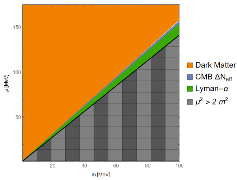
Figure 3: The available parameter space for a DBB when $\mu\gtrsim m$. The bounds have been recast from Fig. 2 to $m$-$\mu$ space using Eqs. 18 and 19. Also plotted is the constraint that $\mu>\sqrt{2\lambda m}$ with $\lambda$=1. The white region shows tunneling field parameter choices for a DBB consistent with the bounds and widens (narrows) beyond the figure to the right (left). While it appears that the parameter space is closed for most of the figure, Fig. 4 will show that the parameter space remains open throughout this range and is too narrow to visualize at this scale.

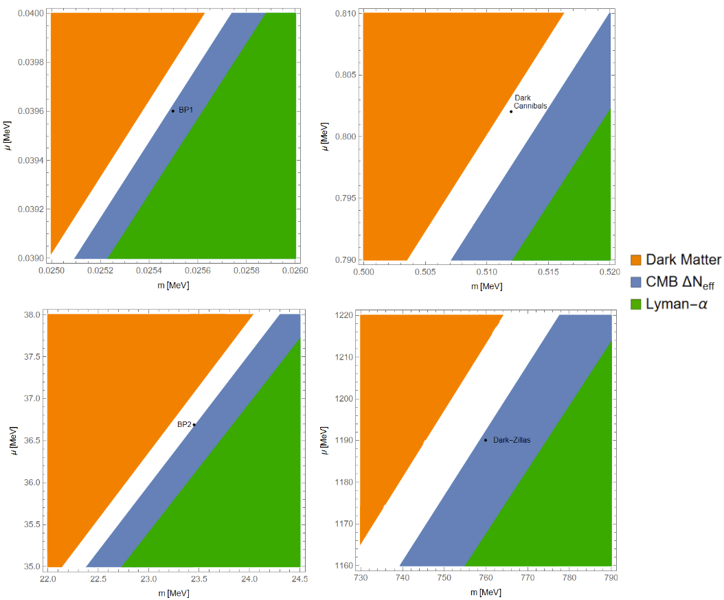
Figure 4: Magnified regions of the sliver parameter space shown in Fig. 3. The regions chosen correspond to the four benchmark Dark Big Bangs considered in [1]. Interestingly, we found that the choices of parameters for BP1 (Panel 1) and Dark-Zillas (Panel 4) violate the upper bound on $\alpha$. We believe this is a result of compounding rounding errors due to sensitivity of this region. These discrepancies do not significantly impact the results of [1], as the parameters can be adjusted slightly to produce the same PT characteristics used in their analysis.

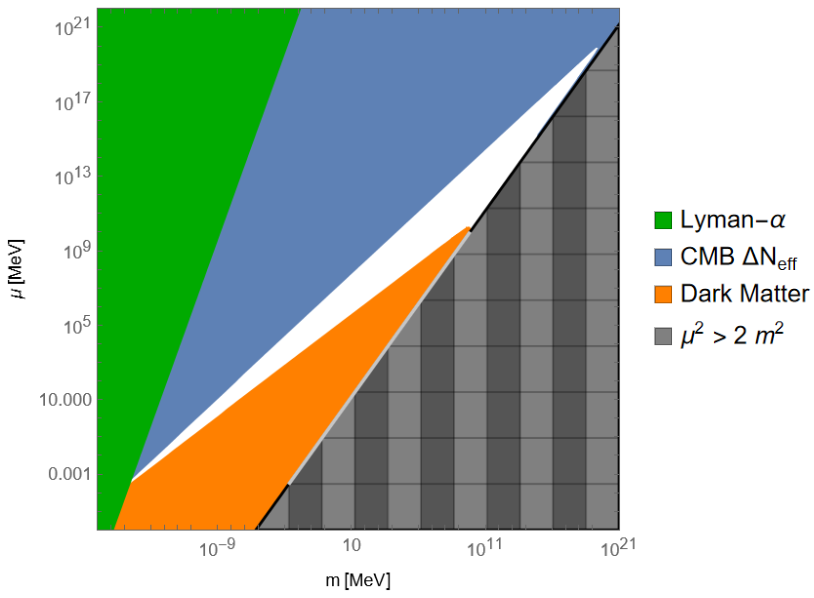
Figure 5: Region 2 of the available parameter space is shown in white with the relevant bounds as in Fig. 2. Using a log scale on both axes, the sliver region is imperceptible but remains open and is represented by the gray boundary line. Above $m\approx 6.1\times 10^{9}$, the lower (orange) bound on $\alpha$ plays no role and the parameter space is bounded on both sides by the upper (blue) bound.

The two separated regions of parameter space are a consequence of the minimum of $\alpha$ at constant $m$ dropping below the lower bound before returning back through the parameter space. As $m$ and $\mu$ increase, the minimum value of $\alpha$ increases. Eventually, the minimum of $\alpha$ crosses above the lower bound and the two parameter spaces merge. Above this point, the parameter space is bounded on both sides by the upper bound on $\alpha$ until not even the minimum value of $\alpha$ crosses below the upper bound. The critical points are summarized in Tab. 1.

Critical Point	($m,\mu$) [MeV]
Region 2 opens	($1.9\times 10^{-16},2.1\times 10^{-4}$)
Region 1 opens	$(2.3160\times 10^{-4},3.5915\times 10^{-4})$
Regions merge	($6.10\times 10^{9},1.64\times 10^{10}$)
Parameter space closes (TCC)	($1.65\times 10^{12},2.70\times 10^{12}$)
Parameter space closes	($8.17\times 10^{19},2.18\times 10^{20}$)

Table 1: Numerical solutions for the critical points of the parameter space in order of increasing $m$. The parameter space is closed below the “opening” values and above the “closing” values. The two different values for where the parameter space closes are from whether or not the Trans-Planckian Censorship Conjecture (TCC) is considered as a bound on the scale of inflation (see Sec. V). The opening point of Region 1 must be approximated to smaller orders of magnitude because of the sensitivity of $\alpha$ near the singularity.

V Discussion

We are particularly interested in looking at the qualitative differences between the two regions. In Region 2, $\mu\gg m$, making analytic analysis much simpler than in the sliver. Additionally, there has yet to be a benchmark DBB considered with input parameters drawn from this region. Given these considerations, this section will first look at the features of tunneling potentials from Region 2 and then consider benchmark DBBs using input parameters from this region.

V.1 Tunneling Potentials

Looking at the quartic potential in Eq. 2, one can deduce the effects $m,\mu$, and $\lambda$ have on the shape of the potential. As $\phi$ increases from zero, $V(\phi)$ first increases $\sim m^{2}\phi^{2}$, then decreases $\sim\mu\phi^{3}$, and finally increases $\sim\lambda\phi^{4}$. So throughout Region 2, where $\mu\gg m$, the potential barrier protecting the stability of the false vacuum is the smallest feature of the tunneling potential, as shown in Fig. 6. This section will show that although $V_{\rm{b}}$ is small throughout Region 2, the tunneling potentials from this region can successfully provide the initial conditions for a first-order phase transition in the dark sector.

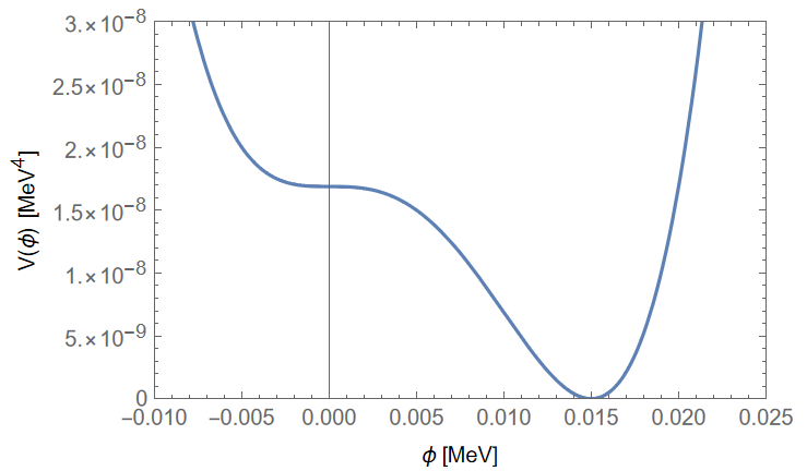
Figure 6: Benchmark tunneling field potential from Region 2 of the parameter space. The potential shown here corresponds to the input parameters of DW 1 shown in Tab. 2. Although the potential barrier is imperceptible, it is large enough to withstand thermal fluctuations. For this potential, $V_{\rm{b}}\sim 10^{-77}$ MeV⁴ while $T_{\rm{GH}}^{4}\sim 10^{-106}$ MeV⁴.

Additional constraints on the tunneling field potential come from the stability of the dark false vacuum. While the tunneling field is trapped in the metastable minimum of the potential, the dark sector goes through a period of inflation. For the dark false vacuum to remain stable during inflation, fluctuations caused by the Gibbons-Hawking temperature $T_{\rm{GH}}$ must not exceed the potential barrier $(T_{\rm{GH}})^{4}\lesssim V_{\rm{b}}$ [1, 24]. The Gibbons-Hawking temperature is proportional to the Hubble parameter during inflation $T_{\rm{GH}}=H_{I}/2\pi$ [25]. We then have the condition

$$V_{\rm{b}}\gtrsim\left(\frac{1}{2\pi}\right)^{4}\left(\frac{\Delta V}{3M_{p}^{2}}\right)^{2}$$ (21)

where the Hubble parameter of the dark sector during inflation is defined with $\rho_{\rm{DS}}=\Delta V$. In Region 2, we can safely use analytic approximations for $V_{\rm{b}}$ and $\Delta V$. It can be shown that for $\mu\gg\rm{m}$,

$$\Delta V\approx\frac{27}{256}\mu^{4}\left(1-\frac{4}{3}\frac{m^{2}}{\mu^{2}}\right)$$ (22)

and

$$V_{\rm{b}}\approx\frac{576m^{6}}{31104\mu^{2}}$$ (23)

Eqs. 22 and 23 show that $\Delta V>V_{\rm{b}}$ throughout Region 2, ensuring the tunneling field will indeed decay and not remain in the false vacuum forever. Yet it is important to check that the barrier height is large enough to remain stable during inflation because of the $V_{\rm{b}}\sim\mu^{-2}$ dependence. Using these approximations, we find that all of Region 2 produces tunneling field potentials with barrier heights large enough to avoid destabilization from fluctuations caused by $T_{\rm{GH}}$, i.e. the Gibbons-Hawking bound is weaker than the upper limit on $\alpha$, as shown in Fig. 7.

Because $m\ll\mu$ throughout Region 2, there appears to be risk of isocurvature perturbations [26] being generated in the dark matter content (see [1] for details). We find that throughout Region 2, $m>H_{I}$ where as before $H_{I}=\sqrt{\frac{\Delta V}{3M_{\rm{p}}^{2}}}$ and $m$ is the mass of the tunneling field in the false vacuum. Therefore isocurvature perturbations are not induced since quantum fluctuations in $\phi$ are heavily suppressed. Fig. 7 shows that imposing the bounds for false vacuum stability (Gibbons-Hawking) and the upper limit on the strength of the DBB (CMB $\Delta N_{\rm{eff}}$) ensure that isocurvature perturbations are safely avoided throughout Region 2.

The most stringent bound on the energy scale of the phase transition is realized through the Trans-Planckian Censorship Conjecture (TCC) [27]. This conjecture postulates an upper limit on the scale of inflation for a consistent theory of quantum gravity [28, 1]

$$\Delta V\lesssim 10^{48}\rm{MeV}^{4}$$ (24)

where $(\Delta V)^{1/4}$ is the energy scale of dark sector inflation. Imposing this bound closes the parameter space at much smaller $m$ and $\mu$ values than in Fig. 5. The parameter space including limits on the scale of inflation from the TCC is shown in Fig. 7.

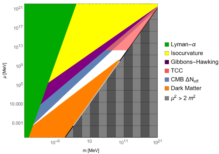
Figure 7: The available parameter space for a DBB consistent with observations, including constraints on the scale of (dark sector) inflation. The open parameter space is the same as Fig. 5 with an additional bound from the Trans-Planckian Censorship Conjecture (TCC), since the bounds from unwanted isocurvature perturbations and false vacuum stability considerations are both weaker than the upper bound on $\alpha$. The TCC bound closes the parameter space above it entirely at the ($m,\mu$) value shown in Tab. 1.

Appendix B shows calculated PT and tunneling field parameters for the critical points in Tab. 1. A notable result of these calculations is that a DBB as late as $\approx$ 32.5 days (the latest a DBB can occur) after the Hot Big Bang can be realized in both Region 1 and Region 2. The only significant difference (for a very late DBB) between these two regions is the mass shift $m$ undergoes in transitioning from the false vacuum to the true vacuum: $\mathcal{O}(1)$ in Region 1, $\mathcal{O}(10^{12})$ in Region 2.

V.2 Benchmark Dark Big Bangs

A large range of dark matter particle masses $m_{\chi}$ can be realized through the DBB [1]. The energy scale of dark sector inflation acts as a guide to the dark matter that can be considered. A dark sector with light dark matter requires $m_{\chi}\lesssim(\Delta V)^{1/4}$. On the other hand, dark matter can be more energetic than the energy scale of dark sector inflation by considering the Lorentz boost of the (runaway) bubble walls $\gamma_{w}$ [1, 29]. Heavy dark matter $m_{\chi}\gg(\Delta V)^{1/4}$ is then limited by [1, 29]

$$m_{\chi}\lesssim\gamma_{w}m_{\phi}\simeq 2\frac{\Delta V}{m(\Delta\phi)^{2}}\frac{M_{\rm{p}}}{\sqrt{g_{\rm{eff}}(T_{*})T_{*}^{4}}}m_{\phi}$$ (25)

The maximum possible dark matter masses for the critical points of the parameter space are shown in Tab. 3. The DBB is constrained to be consistent with the $\Lambda$CDM model of cosmology, so dark matter produced in the DBB must become cold early enough in the universe to reflect the $\Lambda$CDM picture of structure formation. The requirement that dark matter be non relativistic by $T>7.8$ keV [1] somewhat constrains choices of $m_{\chi}$ in constructing a model DBB. While there are many dark matter particle models that can be realized through a DBB [1], we will choose the simplest model: dark WIMPs.

Dark WIMPs are analogous to the well known WIMP model for particle dark matter, the difference being dark WIMPs annihilate into dark radiation $\xi$ that resides in the dark sector [1]. We will choose both $\chi$ and $\xi$ to be real scalars for simplicity (following choices made in Ref. [1]). The Lagrangian is then Eq. 1 with [1]

$$\mathcal{L}_{\rm{DR}}\supset y^{\prime}\chi^{2}\xi^{2}$$ (26)

where we have only included terms important to the annihilation process being considered. For our benchmark cases, we follow the standard thermal freeze out model using [1]

$$\frac{dY_{\chi}}{dT}=\frac{\langle\sigma_{\chi\chi\rightarrow\xi\xi}v\rangle s}{TH(T)}\left(1+\frac{T}{3g_{\rm{eff}}}\frac{dg_{\rm{eff}}}{dT}\right)(Y_{\chi}^{2}-Y_{\chi,eq}^{2})$$ (27)

as the Boltzmann equation for $\chi\chi\leftrightarrow\xi\xi$ annihilations, where $Y_{\chi}=n_{\chi}/s$.

The largest deviations from the freeze out of standard WIMPs come from the dark and visible sectors having different temperatures. In the dark WIMP case, the equilibrium abundance $Y_{\chi,\rm{eq}}$ depends on $T_{\rm{DS}}$, as does when $\chi$ is considered to be relativistic $m_{\chi}/T_{\rm{DS}}>1$. Since entropy is conserved in both sectors and, for the dark WIMP case, the dark sector always has relativistic degrees of freedom, the ratio of the temperatures of the two sectors is constant up to changes in the degrees of freedom [1]

$$\frac{T_{\rm{DS}}}{T}=\left(\frac{g_{\rm{eff}}(T)}{g_{\rm{eff}}(T_{*})}\right)^{1/3}\left(\frac{g_{\rm{DS}}(T_{\rm{DS,*}})}{g_{\rm{DS}}(T_{\rm{DS}})}\right)^{1/3}\frac{T_{\rm{DS,*}}}{T_{*}}$$ (28)

Eq. 28 can be used to put $T_{\rm{DS}}$ in terms of $T$. For the benchmark cases considered here, we took $g_{\rm{DS},*}=2$ if $\chi$ is produced relativistically and $g_{\rm{DS}}=1$ once $\chi$ becomes non-relativistic ($\xi$ will always contribute to the dark sector degrees of freedom). In our calculations, we approximated $g_{\rm{DS}}$ with a continuous step function of the form

$$g_{\rm{DS}}(T)\approx\frac{g_{\rm{DS},f}-g_{\rm{DS},i}}{e^{(T-T_{\rm{nr}})/K}+1}+g_{\rm{DS},i}$$ (29)

where $g_{\rm{DS},i}$ $(g_{\rm{DS},f})$ is the initial (final) relativistic degrees of freedom in the dark sector, $T_{\rm{nr}}$ is the visible sector temperature at which $\chi$ becomes non relativistic ($m_{\chi}/T_{\rm{DS}}=1$), and K is a constant determining how fast $\chi$ becomes non-relativistic. The benchmark cases considered are shown in Tab. 2.

Benchmark	DW 1	DW 2
Input Parameters
$m_{\chi}$ [keV]	10	500
$m$ [keV]	$8\times 10^{-11}$	$6\times 10^{-5}$
$\mu$ [keV]	20	$2.00\times 10^{5}$
$y^{\prime}\times 10^{7}$	$0.0120$	0.189
$\lambda$	1	1
$K$	0.012	0.34
Derived Parameters
$m_{\phi}$ [keV]	30.0	3.00 $\times 10^{5}$
$(\Delta V)^{1/4}$ [keV]	11.4	$1.14\times 10^{5}$
Phase Transition
$t_{*}$ [s]	1545	$2.75\times 10^{-5}$
$T_{*}$ [MeV]	0.029	138.39
$T_{\rm{DS,*}}$ [MeV]	0.013	126.55
$\alpha$	0.02	0.07
Dark Matter
$\langle\sigma_{\chi\chi\rightarrow\xi\xi}v\rangle$ [$\rm{cm^{3}s^{-1}}$]	$1.3\times 10^{-26}$	$1.3\times 10^{-27}$
$T_{\rm{nr}}$ [keV]	18.4	553.32
$T_{\rm{FO}}$ [keV]	2.37	62.78
$\Omega_{\chi}h^{2}$	0.120	0.120
$\Delta N_{\rm{eff}}$	0.24	0.41

Table 2: Benchmark Dark Big Bangs producing Dark WIMP (DW) dark matter with input parameters from Region 2. The input parameters were chosen to feature phase transitions that occur at different times in the universe, are strong enough to fall within the sensitivity bounds of upcoming GW surveys, and produce the correct relic abundance assuming Dark WIMPs make up all the dark matter in the universe. Benchmark cases featuring the same Dark WIMP masses with parameters chosen from Region 1 can be found in Ref. [1].

The evolution of $\rho_{\chi}$ for each benchmark case is shown in Fig. 8. Once $Y_{\chi}$ is solved for numerically, the dark WIMP energy density is given by $\rho_{\chi}=m_{\chi}Y_{\chi}s$ in the non relativistic regime. The dark WIMP energy density evolution while the particles are in thermal equilibrium and (for the most part) relativistic is

$$\rho_{\chi,\rm{eq}}=\frac{g_{\rm{DS}}(T)}{2\pi^{2}}m_{\chi}^{3}T_{\rm{DS}}K_{1}\left(\frac{m_{\chi}}{T_{\rm{DS}}}\right)+T_{\rm{DS}}Y_{\chi,\rm{eq}}s$$ (30)

where $K_{1}$ is a modified Bessel function of the second kind and $s$ is the entropy density of the visible sector $s=\frac{2\pi^{2}}{45}g_{\rm{s}}(T)T^{3}$. Eq. 30 is found by numerically integrating the Maxwell-Boltzmann phase space distributions for $n_{\chi,\rm{eq}}$ and $\rho_{\chi,\rm{eq}}$.

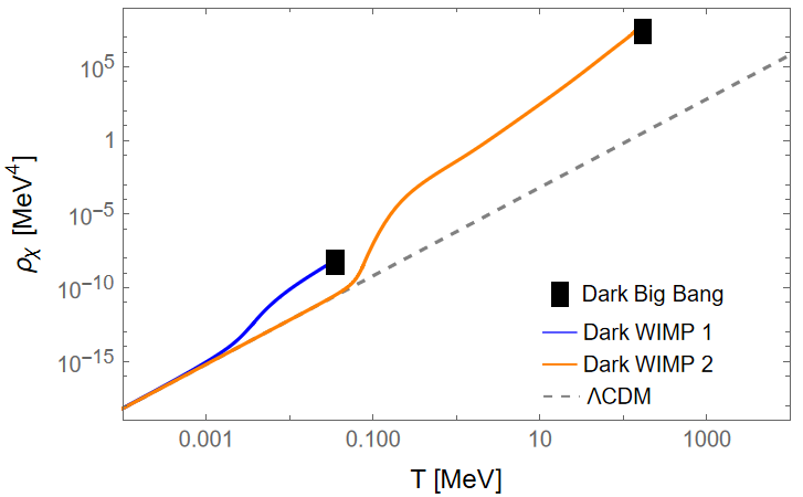
Figure 8: Evolution of the Dark WIMP energy density for the two benchmark cases shown in Tab. 2. In both cases, the dark matter is produced relativistically and redshifts like $\rho_{\chi}\propto T^{4}$. The Dark WIMPs freeze out as cold relics and join the standard $\Lambda$CDM evolution track, redshifting like $\rho_{\chi}\propto T^{3}$ and producing the correct relic abundance of dark matter in the late universe.

Before the DBB, all of the energy in the dark sector resides in the tunneling field $\phi$. After the DBB, the energy is split between dark matter particles, dark radiation, and gravity waves. The energy density of the gravity waves produced during the DBB can be approximated by [30, 1]

$$\rho_{\rm{GW,*}}\sim 0.05\hskip 1.42262pt\alpha\hskip 1.42262pt\Delta V$$ (31)

at the time of the DBB. The energy density of gravity waves will redshift like $\rho_{\rm{GW}}\sim a^{-4}$ [1]. The projected sensitivity windows of the International Pulsar Timing Array (IPTA) [31] and the Square Kilometer Array (SKA) [32] make strong and late DBB’s favorable for detection [1]. Both benchmark Dark Big Bangs fall withing IPTA and SKA sensitivity windows.

VI Conclusion

The Dark Big Bang is an exciting new theory for the evolution of the universe. As WIMPs continue to evade detection, it is becoming increasingly important to consider dark sectors that are strongly decoupled from the visible sector. We have conducted an extensive analysis of the available parameter space for the tunneling potential of a DBB that is consistent with cosmological observations. Notably, we have shown that a region of parameter space exists (Region 2) far from the singularity of the Euclidean action. This region of parameter space is especially useful because many of the PT parameters can be determined through analytic approximations.

We have shown that nearly all of the important characteristics describing a DBB can be put in terms of the tunneling field parameters $m$, $\mu$, and $\lambda$. Even the gravity waves released from the PT, one of the most important observables of the DBB, can be determined from the tunneling field parameters (Eq. 31). Evidence for the existence of a stochastic background of gravity waves permeating the universe was first detected by NanoGrav in June 2023 [12]. As research on gravity waves continues to advance, signatures of a DBB may become differentiable from the stochastic background. In fact, signatures of the Dark Big Bang may have already been observed in NanoGrav’s 15 year data set [1].

In the future, it would be interesting to see how the projected sensitivities of upcoming gravity wave surveys translate onto the parameter space of the tunneling field potential. Future research could also consider weak couplings between the dark and visible sectors through portals. These couplings could give rise to additional observable signatures of the DBB [1] and new bounds on the tunneling field potential parameters.

Appendix A Analytic Behavior

In this section we discuss the analytic behavior of the phase transition parameters. We will separate the parameter space into two regimes: Region 1 ($\mu\gtrsim$ m) and Region 2 ($\mu\gg$ m).

A.1 Region 1

Both $\alpha$ and $T_{*}$ depend on the Euclidean action of the bounce solution. In the thin wall approximation, which is good enough to understand the general behavior

$$S\approx\frac{\pi^{2}\mu^{6}}{24\lambda(\mu^{2}-2\lambda m^{2})^{3}}$$ (32)

S has a singularity at $\mu^{2}=2\lambda m^{2}$, which is the driving factor for the behavior of $\alpha$ and $T_{*}$ for Dark Big Bangs where $m$ and $\mu$ are comparable in size. Since $\mu>\sqrt{2\lambda}m$, we are right above the singularity in this region of parameter space. Setting $\lambda=1$, $\alpha$ scales like:

$$\alpha\sim m^{-2}S^{-1}e^{S/2}\Delta V$$ (33)

Here we can ignore the $\Delta V$ term, since the singularity of S drives the behavior. Above the singularity, $\alpha$ decreases rapidly from positive infinity. The scaling of $T_{*}$ is

$$T_{*}\sim(m^{4}S^{2}e^{-S})^{1/8}$$ (34)

Above the singularity, $T_{*}$ initially increases from zero, dominated by $S^{2}$, then decreases like $e^{-S}$. These scaling show that, in Region 1, the phase transition parameters are extremely sensitive to the values of $m$ and $\mu$. Being near the singularity means there is a very narrow parameter space in which $\alpha$ and $T_{*}$ both fall within the correct bounds.

A.2 Region 2

Another allowed parameter space for a DBB consistent with the imposed bounds opens up when $\mu\gg m$ for reasons that will be shown here. In this region we are far from the singularity. It is convenient to rewrite the tunneling potential and PT parameters in terms of the variable $\frac{m^{2}}{\mu^{2}}$. In the following analysis, we set higher order terms of $\frac{m^{2}}{\mu^{2}}$ to zero and set $\lambda=1$. To first-order approximation, the Euclidean action scales like

$$S\sim 1-6\frac{m^{2}}{\mu^{2}}$$ (35)

and the potential difference scales like

$$\Delta V\sim\mu^{4}(1-\frac{8}{3}\frac{m^{2}}{\mu^{2}})$$ (36)

Using these approximations and Eq. 33, it can be shown that for $\mu\gg m$,

$$\alpha\sim\frac{\mu^{6}}{m^{4}}$$ (37)

and using Eq. 34

$$T_{*}\sim\frac{m}{\mu^{1/2}}$$ (38)

These scalings show that region 2 of the parameter space should be expected. Near the singularity, $\alpha$ decreases from positive infinity, shooting quickly through the allowed parameter space. Then, if $m$ is fixed and $\mu$ increased, $\alpha$ will return to allowed values from below the lower bound.

We can also find the slope of the bounds on the DBB when $\mu\gg m$. Writing the lower bound on $\alpha$ (CMB $\Delta N_{\rm{eff}}$) as a function of $\mu$, we find

$$\mu\sim m^{6/11}$$ (39)

For the upper bound on $\alpha$ (Dark Matter), we find

$$\mu\sim m^{2/3}$$ (40)

These scaling relations are reflected in the parameter space where the upper bound on $\alpha$ has a steeper slope than the lower bound (see Fig. 5 or Fig. 7). The steepest slope is the temperature (Lyman-$\alpha$) bound which has the scaling $\mu\sim m^{2}$, as can be seen from Eq. 38.

Appendix B Critical Point Evaluation

The purpose of this section is to give numerical values for the tunneling field potentials and phase transition parameters for critical points tabulated in Tab. 1. Since the critical points found are numerical approximations for the boundaries of the parameter space, some values calculated violate the bounds imposed on the DBB and some fall just within the parameter space. Tab. 3 is meant to give a general idea of the tunneling field and PT parameters near the critical points. For all calculations, we set $\lambda=1$.

	R2 Opens	R1 Opens	Intersection	PS Closes (TCC)	PS Closes
$m$ [MeV]	$1.90\times 10^{-16}$	$2.3160\times 10^{-4}$	$6.10\times 10^{9}$	$1.65\times 10^{12}$	$8.17\times 10^{19}$
$\mu$ [MeV]	$2.10\times 10^{-4}$	$3.5915\times 10^{-4}$	$1.64\times 10^{10}$	$2.70\times 10^{12}$	$2.18\times 10^{20}$
($\Delta V)^{1/4}$ [MeV]	$1.20\times 10^{-4}$	$1.20\times 10^{-4}$	$8.41\times 10^{9}$	$1.01\times 10^{12}$	$1.12\times 10^{20}$
$\Delta\phi$ [MeV]	$1.58\times 10^{-4}$	$2.03\times 10^{-4}$	$1.15\times 10^{10}$	$1.60\times 10^{12}$	$1.53\times 10^{30}$
($V_{b})^{1/4}$ [MeV]	$7.75\times 10^{-5}$	$7.55\times 10^{-5}$	$1.41\times 10^{9}$	$5.17\times 10^{11}$	$1.89\times 10^{19}$
$m_{\phi}$ [MeV]	$3.15\times 10^{-4}$	$3.35\times 10^{-4}$	$2.22\times 10^{10}$	$2.74\times 10^{12}$	$2.94\times 10^{20}$
$t_{*}$ [s]	$2.88\times 10^{6}$	$2.86\times 10^{6}$	$6.13\times 10^{-31}$	$4.62\times 10^{-25}$	$4.66\times 10^{-41}$
$T_{*}$ [MeV]	$6.78\times 10^{-4}$	$6.81\times 10^{-4}$	$6.19\times 10^{14}$	$7.13\times 10^{11}$	$7.09\times 10^{19}$
$T_{\rm{DS,*}}$ [MeV]	$1.33\times 10^{-4}$	$1.32\times 10^{-4}$	$9.33\times 10^{9}$	$1.11\times 10^{12}$	$1.24\times 10^{20}$
$\alpha$	$8.77\times 10^{-4}$	$8.50\times 10^{-4}$	$9.69\times 10^{-22}$	$0.113$	0.170
$m_{\chi,\rm{max}}$ [GeV]	$7.94\times 10^{28}$	$4.04\times 10^{16}$	$1.69\times 10^{8}$	$6.16\times 10^{17}$	$2.24\times 10^{18}$

Table 3: Tunneling potential and phase transition parameters for the critical points in the $m-\mu$ parameter space. To calculate $T_{\rm{DS},*}$, we fixed $g_{\rm{DS}}=2$. We have also included the maximum mass of dark matter candidates produced in each DBB scenario, according to Eq. 25. For the critical point where Region 2 (R2) opens (column 2), T_∗ is slightly below the Lyman-$\alpha$ bound. Notably, for both critical points where the parameter space (PS) closes (columns 5 & 6), $T_{\rm{DS},*}>T_{*}$ yet $\alpha$ falls within the bounds (it is typical for the dark sector reheating temperature to be less than the visible sector temperature at the DBB). This is a result of our choice for $g_{\rm{DS}}$, which is much smaller than $g_{\rm{eff}}$ at high temperatures.

References

- Freese and Winkler [2023] K. Freese and M. W. Winkler, Dark matter and gravitational waves from a dark big bang, Phys. Rev. D 107, 083522 (2023).
- Zwicky [1933] F. Zwicky, Die rotverschiebung von extragalaktischen nebeln, Helvetica Physica Acta, Vol. 6, p. 110-127 6, 110 (1933).
- Einasto et al. [1974] J. Einasto, A. Kaasik, and E. Saar, Dynamic evidence on massive coronas of galaxies, Nature 250, 309 (1974).
- Ostriker et al. [1974] J. Ostriker, P. Peebles, and A. Yahil, The size and mass of galaxies and the mass of the universe (1974).
- Ostriker and Peebles [1973] J. P. Ostriker and P. J. Peebles, A numerical study of the stability of flattened galaxies: or, can cold galaxies survive?, The Astrophysical Journal 186, 467 (1973).
- Aghanim et al. [2020] N. Aghanim, Y. Akrami, M. Ashdown, J. Aumont, C. Baccigalupi, M. Ballardini, A. Banday, R. Barreiro, N. Bartolo, S. Basak, et al., Planck 2018 results-vi. cosmological parameters, Astronomy & Astrophysics 641, A6 (2020).
- Bertone and Hooper [2018] G. Bertone and D. Hooper, History of dark matter, Reviews of Modern Physics 90, 045002 (2018).
- Berlin and Kling [2019] A. Berlin and F. Kling, Inelastic dark matter at the lhc lifetime frontier: Atlas, cms, lhcb, codex-b, faser, and mathusla, Physical Review D 99, 015021 (2019).
- Akerib et al. [2020] D. Akerib, C. Akerlof, S. Alsum, H. Araújo, M. Arthurs, X. Bai, A. Bailey, J. Balajthy, S. Balashov, D. Bauer, et al., Projected wimp sensitivity of the lux-zeplin dark matter experiment, Physical Review D 101, 052002 (2020).
- Ade et al. [2019] P. Ade, J. Aguirre, Z. Ahmed, S. Aiola, A. Ali, D. Alonso, M. A. Alvarez, K. Arnold, P. Ashton, J. Austermann, et al., The simons observatory: science goals and forecasts, Journal of Cosmology and Astroparticle Physics 2019 (02), 056.
- Abazajian et al. [2019] K. Abazajian, G. Addison, P. Adshead, Z. Ahmed, S. W. Allen, D. Alonso, M. Alvarez, A. Anderson, K. S. Arnold, C. Baccigalupi, et al., Cmb-s4 science case, reference design, and project plan, arXiv preprint arXiv:1907.04473 (2019).
- Agazie et al. [2023] G. Agazie, A. Anumarlapudi, A. M. Archibald, Z. Arzoumanian, P. T. Baker, B. Bécsy, L. Blecha, A. Brazier, P. R. Brook, S. Burke-Spolaor, et al., The nanograv 15 yr data set: Evidence for a gravitational-wave background, The Astrophysical Journal Letters 951, L8 (2023).
- Adhikari et al. [2019] G. Adhikari, P. Adhikari, E. B. de Souza, N. Carlin, S. Choi, M. Djamal, A. Ezeribe, C. Ha, I. Hahn, E. J. Jeon, et al., Search for a dark matter-induced annual modulation signal in nai (tl) with the cosine-100 experiment, Physical review letters 123, 031302 (2019).
- Cushman et al. [2013] P. Cushman, C. Galbiati, D. McKinsey, H. Robertson, T. Tait, D. Bauer, A. Borgland, B. Cabrera, F. Calaprice, J. Cooley, et al., Snowmass cf1 summary: Wimp dark matter direct detection, arXiv preprint arXiv:1310.8327 (2013).
- O’Hare [2021] C. A. O’Hare, New definition of the neutrino floor for direct dark matter searches, Physical Review Letters 127, 251802 (2021).
- Coleman [1977] S. Coleman, Fate of the false vacuum: Semiclassical theory, Physical Review D 15, 2929 (1977).
- Baumann [2022] D. Baumann, Cosmology (Cambridge University Press, 2022).
- Garzilli et al. [2021] A. Garzilli, A. Magalich, O. Ruchayskiy, and A. Boyarsky, How to constrain warm dark matter with the lyman- forest, Monthly Notices of the Royal Astronomical Society 502, 2356 (2021).
- Villasenor et al. [2023] B. Villasenor, B. Robertson, P. Madau, and E. Schneider, New constraints on warm dark matter from the lyman- forest power spectrum, Physical Review D 108, 10.1103/physrevd.108.023502 (2023).
- Callan Jr and Coleman [1977] C. G. Callan Jr and S. Coleman, Fate of the false vacuum. ii. first quantum corrections, Physical Review D 16, 1762 (1977).
- Kolb [2018] E. Kolb, The early universe (CRC press, 2018).
- Adams [1993] F. C. Adams, General solutions for tunneling of scalar fields with quartic potentials, Physical Review D 48, 2800 (1993).
- Freese and Winkler [2022] K. Freese and M. W. Winkler, Have pulsar timing arrays detected the hot big bang: Gravitational waves from strong first order phase transitions in the early universe, Physical Review D 106, 103523 (2022).
- Hawking and Moss [1982] S. W. Hawking and I. L. Moss, Supercooled phase transitions in the very early universe, Physics Letters B 110, 35 (1982).
- Gibbons and Hawking [1977] G. W. Gibbons and S. W. Hawking, Cosmological event horizons, thermodynamics, and particle creation, Physical Review D 15, 2738 (1977).
- Kofman and Linde [1987] L. A. Kofman and A. D. Linde, Generation of density perturbations in inflationary cosmology, Nuclear Physics B 282, 555 (1987).
- Bedroya and Vafa [2020] A. Bedroya and C. Vafa, Trans-planckian censorship and the swampland, Journal of High Energy Physics 2020, 1 (2020).
- Bedroya et al. [2020] A. Bedroya, R. Brandenberger, M. Loverde, and C. Vafa, Trans-planckian censorship and inflationary cosmology, Physical Review D 101, 103502 (2020).
- Watkins and Widrow [1992] R. Watkins and L. M. Widrow, Aspects of reheating in first-order inflation, Nuclear Physics B 374, 446 (1992).
- Caprini et al. [2007] C. Caprini, R. Durrer, and G. Servant, Gravitational wave generation from bubble collisions in first-order phase transitions: An analytic approach, arXiv preprint arXiv:0711.2593 (2007).
- Antoniadis et al. [2022] J. Antoniadis, Z. Arzoumanian, S. Babak, M. Bailes, A. Bak Nielsen, P. Baker, C. Bassa, B. Bécsy, A. Berthereau, M. Bonetti, et al., The international pulsar timing array second data release: Search for an isotropic gravitational wave background, Monthly Notices of the Royal Astronomical Society 510, 4873 (2022).
- Dewdney et al. [2009] P. E. Dewdney, P. J. Hall, R. T. Schilizzi, and T. J. L. Lazio, The square kilometre array, Proceedings of the IEEE 97, 1482 (2009).