London SW7 2AZ UK
22email: p.bressloff@imperial.ac.uk
Cellular diffusion processes in singularly perturbed domains
Abstract
There are many processes in cell biology that can be modeled in terms of particles diffusing in a two-dimensional (2D) or three-dimensional (3D) bounded domain containing a set of small subdomains or interior compartments , (singularly-perturbed diffusion problems). The domain could represent the cell membrane, the cell cytoplasm, the cell nucleus or the extracellular volume, while an individual compartment could represent a synapse, a membrane protein cluster, a biological condensate, or a quorum sensing bacterial cell. In this review we use a combination of matched asymptotic analysis and Green’s function methods to solve a general type of singular boundary value problems (BVP) in 2D and 3D, in which an inhomogeneous Robin condition is imposed on each interior boundary . This allows us to incorporate a variety of previous studies of singularly perturbed diffusion problems into a single mathematical modeling framework. We mainly focus on steady-state solutions and the approach to steady-state, but also highlight some of the current challenges in dealing with time-dependent solutions and randomly switching processes.
1 Introduction
There are a wide range of problems in cell biology that can be modelled in terms of particles diffusing in a two-dimensional (2D) or three-dimensional (3D) bounded domain containing a set of small subdomains or compartments , , within the interior (singularly-perturbed diffusion problems). For example, could represent the cell membrane while the compartments could represent synapses or protein clusters such as macro-assemblies of adhesion molecules. Alternatively, if were the cell volume then the corresponding compartments could be enzyme-rich reactive substrates, or high density liquid droplets (biological condensates). On a larger length scale, could represent the extracellular medium surrounding a set of diffusively-coupled cells as in bacterial quorum sensing. In most of these applications one is interested in calculating the steady-state solution (assuming it exists), and the rate of approach to steady state as determined by the principal eigenvalue of the linear evolution operator or by the so-called accumulation time111Another class of problem treats the compartments as totally or partially absorbing traps, and the main focus is determining the first passage time or splitting probability for a single particle to be captured by one of the traps – the so-called narrow capture problem Coombs09 ; Chevalier11 ; Coombs15 ; Ward15 ; Lindsay16 ; Lindsay17 ; Grebenkov20 ; Bressloff21a ; Bressloff21b . We do not consider single particle diffusion in this review.. The latter is based on the fractional deviation of the time-dependent solution from steady state, and has been used extensively in studies of diffusion-based morphogenesis Berez10 ; Berez11 ; Berez11a ; Gordon11 ; Bressloff19 . The type of steady-state boundary value problem (BVP) that typically arises can be analysed using a combination of matched asymptotic analysis and Green’s function methods. The basic idea is to construct an inner or local solution of the diffusion equation in a small neighbourhood of each compartment, which is then matched to an outer solution in the bulk domain. The matching is achieved by expressing the outer solution in terms of the Green’s function of the diffusion equation in the absence of any compartments. It follows that the details of the matched asymptotic analysis in 2D and 3D domains differ considerably due to corresponding differences in the Green’s function singularities:
as . Hence, an asymptotic expansion of the solution to a BVP in 3D is in powers of , where represents the size of a compartment relative to the size of the bulk domain. On the other hand, the analogous expansion in 2D tends to be in powers of at in . The slower convergence of in the limit can be handled by summing the logarithmic terms non-perturbatively, as originally shown in Refs. Ward93 ; Ward93a .
Examples of cellular processes that have been analyzed using singular perturbation theory include the following: intracellular protein concentration gradients mediated by enzyme-rich subcellular domains Straube09 ; Levy11 ; Levy13 ; coarsening of biological condensates via Ostwald ripening Kavanagh14 ; Bressloff20a ; Bressloff20b ; Bressloff24b ; protein clustering Bressloff24b ; synaptic receptor trafficking Bressloff08 ; Bressloff23a ; bacterial quorum sensing Muller13 ; Gou16 ; Iyan21a ; Iyan21b ; volume transmission Lawley18 ; Lawley20 . Although each of these applications utilises the same basic mathematical method, they tend to be treated in isolation. Therefore, in this review we show how the majority of current applications can be incorporated into a single type of BVP involving an inhomogeneous Robin boundary condition on combined with the insertion and removal of particles within . We consider three different models for the boundary inhomogeneity : (I) is a prescribed constant on ; (II) acts as a semi-permeable membrane and is identified with the particle concentration on the interior side of the membrane; (iii) is treated as a well-mixed biochemical compartment that can exchange one molecular species with the exterior environment., whose concentration within determines . For simplicity, we assume that all of the compartments are either circularly symmetric (2D) or spherically symmetric (3D). More general shapes are briefly discussed in section 6.
The structure of the paper is as follows222In this review we focus on the underlying mathematical principles and techniques, and how they are applied to singularly-perturbed diffusion problems in cell biology. Explicit results for specific configurations of and , , and choices of boundary conditions can be found in the cited literature.. In section 2 we introduce the general model equations and show how they are related to the various applications in specific limits. In section 3 we solve the steady-state BVP in both 2D and 3D using singular perturbation theory. The relaxation to steady-state is analysed in section 4 by solving the BVP for the singularly perturbed diffusion equations in Laplace space and then taking the small- limit, where is the Laplace variable. This determines the corresponding accumulation time. In section 5 we summarise a recent study Iyan21b that uses singular perturbation theory to reduce a PDE-ODE model of diffusively coupled biochemical compartments (model III) to a nonlinear system of ODEs. Finally, in section 6, we describe various extensions of the theory, including randomly switching boundaries, and Kuramoto-like models of diffusively coupled oscillators. These examples highlight one major challenge for future work on singularly-perturbed diffusion problems, namely, developing asymptotic and numerical methods that can deal effectively with time-dependent and switching processes. (For very recent progress in this direction see Ref. Pelz24 .)
2 The general setup
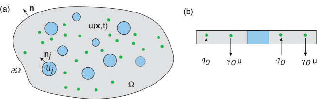
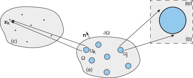
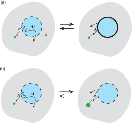
Consider a -dimensional simply-connected, bounded domain , , containing a set of interior subdomains or compartments , , see Fig. 1(a). For concreteness, suppose that each compartment is circularly (spherically) symmetric for () – more general shapes will be considered in section 6. Denoting the radius and centre of the -th compartment by and , respectively, we have
| (2.1) |
The main characteristic of a singularly perturbed domain is that the compartments are small compared to the size of the domain and are well separated. More precisely, suppose that the domain is inscribed by a rectangular area or volume whose smallest dimension is , and introduce the dimensionless parameter where . We then fix length scales by setting and writing with , and . We also assume that for all and , . (If is unbounded, then we identify with the smallest distance between any pair of compartments, that is, .)
Let denote the particle concentration in the region exterior to all of the compartments, that is, with . We take to satisfy the following singularly perturbed diffusion problem:
| (2.2a) | ||||
| (2.2b) | ||||
| (2.2c) | ||||
where is the diffusivity, is the outward unit normal of the exterior surface and is the unit normal of the interior surface that is directed out of the interior , see Fig. 1(a). The term in equation (2.2a) represents a particle source current, whereas the term represents removal of particles at a rate , see Fig. 1(b); the latter could correspond to a degradation rate. The exterior boundary is assumed to be totally reflecting, whereas on each interior boundary we impose a generalised Robin boundary condition with constant reactivity . In the limit , equation (2.2c) reduces to the inhomogeneous Dirichlet boundary condition for all , whereas we obtain a totally reflecting boundary condition when . It remains to specify the boundary field , . We consider three different compartmental models for , as illustrated in Fig. 2:
I. Constant boundary fields. The simplest boundary condition is for all , where is a prescribed constant. Equation (2.2c) then reduces to a classical Robin boundary condition for .
II. Spatially inhomogeneous compartments and semi-permeable interfaces. Now suppose that the boundary acts as a semipermeable interface between diffusion in the exterior domain and diffusion within each interior . Equations (2.2a,b) are supplemented by the following diffusion equation for the particle concentration in :
| (2.3a) | ||||
| and the boundary condition (2.2c) is replaced by the pair of semipermeable boundary conditions | ||||
| (2.3b) | ||||
Here indicates whether a point on the boundary is approached from the exterior or interior of the compartment . The diffusivity within the -th compartment may differ from the exterior diffusivity . We also allow for the insertion and removal of particles within .
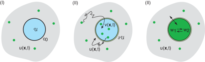
III. Spatially homogeneous compartments as biochemical reaction networks. Each compartment is treated as a biochemical reaction network involving a set of chemical species , . Diffusion within is assumed to be sufficiently fast so that the corresponding compartment can be treated as well-mixed. This means that the concentrations within are spatially homogeneous. Only one of the chemical species can be exchanged with the exterior domain , which we identify with . This implies that for all . Using mass action kinetics we then have the following system of equations for the concentrations :
| (2.4) |
for . For simplicity, the mass action kinetics is taken to be the same for all cells, that is, the form of is independent of .) One can view equations (2.2) and (2.4) with as a nonlinear PDE-ODE model of diffusion-mediated communication between small signalling compartments Gou16 ; Iyan21a ; Iyan21b . Finally, note that the factor of ensures that the number of particles crossing is consistent with the definition of the flux in the boundary condition (2.2c), assuming that the compartmental and bulk concentrations are defined with respect to the same volume.
We now summarise various biological applications of equations (2.2) that involve one of the above compartmental models.
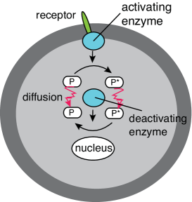
Intracellular signalling Straube09 ; Levy11 ; Levy13 . An important component of many intracellular signal transduction pathways is the reversible cycling between an inactive and an active protein state, which is catalysed by opposing activator and deactivator enzymes. A concentration gradient in these signalling cycles can then be generated by the spatial segregation of the opposing enzymes Brown99 ; Kholodenko09 ; Garcia10 ; Howard12 . One such mechanism is the phosphorylation of proteins by a membrane-bound kinase, which are then dephosphorylated by a cytosolic phosphatase, see Fig. 3. This results in a gradient of the phosphorylated protein, with a high concentration close to the cell membrane and a low concentration within the interior of the cell. As the cell grows in size, the surface-to-volume ratio decreases and membrane-activated proteins have to diffuse over longer distances in order to reach their target such as the nucleus. Hence, the proteins become progressively deactivated towards the cell interior, thus providing a mechanism for coupling cell growth with the cell cycle and cell division Meyers06 . It has also been observed that the range of an intracellular protein gradient can be enhanced by signalling cascades mediated by kinases located on the membranes of subcellular compartments. Cascades of intracellular phosphorylation-dephosphorylation gradients can be formulated in terms of equations (2.2) for and (model I) Straube09 ; Levy11 ; Levy13 . The boundaries represent the membranes of subcellular compartments that are rich in kinases, and is the concentration of an activated signalling molecule in the cytosol. Phosphotases within the cytosol deactivate the signalling molecules at the constant rate . If the total cytosolic concentration of activated and deactivated signalling molecules is a constant and the enzymes on are unsaturated, then one can identify with and with the rate of phosphorylation.
Ostwald ripening of biological condensates Alikakos04 ; Kavanagh14 ; Bressloff20a ; Bressloff20b ; Bressloff24b . Ostwald ripening describes the coarsening of polydisperse droplets during late-stage liquid-liquid phase separation, ultimately transitioning to a single condensate in thermodynamic equilibrium with a surrounding dilute phase Lif61 ; Wagner61 . In this example represents a liquid droplet in the high density phase, is the concentration of particles in the low density phase, and . The boundary condition on each surface is taken to be with
| (2.5) |
where is the density of the dilute phase under complete phase separation, and is the so-called capillary length constant. (More precisely, denotes a volume fraction.) Equation (2.5) expresses the Gibbs-Thomson law due to interfacial tension on the droplet interface Doi13 . We thus have an example of model I in the limit . The no-flux boundary condition on ensures mass conservation. Suppose that the coarsening dynamics is much slower than the equilibration of the concentration profile in the dilute phase. Under this quasi-static approximation, the solute concentration exterior to the droplets satisfies a steady-state diffusion equation of the form
| (2.6) |
The quasi-static approximation ensures that the total volume of condensates is conserved. This follows from integrating equation (2.6a) with respect to and using the divergence theorem:
| (2.7) |
That is, the sum of the fluxes into the condensates is zero so that there is no net change in the total condensate volume. The particle flux at the surface determines the rate of growth or shrinkage of the droplet under the adiabatic approximation. Introduce a slow time-scale and let be the slowly varying radius of the -th droplet. The number of particles within the -th droplet then evolves according to the equation
| (2.8) |
where is the steady-state concentration for the set of radii , and is the corresponding droplet boundary. In the case of a uniform spherical droplet in the high density phase , the number of particles is . Hence, equation (2.8) yields a closed equation for the dynamics of the droplet radii.
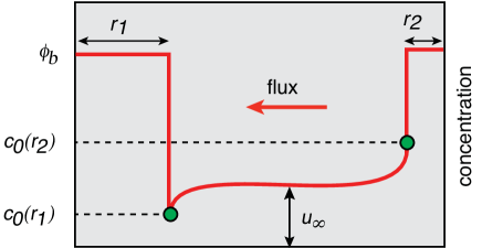
In classical Ostwald ripening, the difference in surface concentrations for droplets of different sizes results in a net diffusive flux from small to large droplets. This is illustrated in Fig. 4 for two droplets and with . These fluxes modify the far-field solute concentration , which ultimately leads to complete phase separation333Standard treatments of Ostwald ripening use a mean-field approximation, in which each droplet “sees” an effective far-field concentration that is determined self-consistently. The theory of diffusion in singularly perturbed domains can be used to calculate corrections to mean field theory Kavanagh14 ; Bressloff20a ; Bressloff20b ; Bressloff24b .. However, multiple coexisting biological condensates are found in the cytoplasm and cell nucleus (see the reviews Hyman14 ; Brangwynne15 ; Berry18 ; Mittag22 and references therein). These membrane-less organelles are viscous, liquid-like structures containing enhanced concentrations of various proteins and RNA, many of which can be continually exchanged with the surrounding medium. It has been hypothesised that the coexistence of multiple droplets over significant timescales involves the active suppression of Ostwald ripening. Various hypotheses have been given to account for this suppression: actively driven chemical reactions that maintain the out-of-equilibrium switching of proteins between soluble and phase separating forms Zwicker15 ; Wurtz18 ; Lee19 ; Weber19 (see also section 6.2); the mechanical suppression of coarsening mediated by intracellular visco-elastic networks such as the cytoskeleton Feric13 ; Style18 ; Ros20 ; the slow conversion of a molecular constituent between the dilute and dense phases due to various regulatory interfacial proteins Seydoux18 ; Folk21 ; Lee21 . The last mechanism can be implemented by considering model I with Bressloff24a .
Protein clustering in membranes Bressloff24b . A second example of a self-organising process based on model I is protein clustering in cell membranes, where is an anchored protein cluster and is the concentration of free proteins. Each boundary is taken to be totally absorbing, and proteins are exchanged between the cytosol and membrane via the active mechanisms of endocytosis and exocytosis Foret12 . That is, and specify the rates of endocytosis and exocytosis, respectively. The aggregation or clustering of proteins and other macromolecules plays an important role in the formation of various large-scale structures in cell membranes, including the assemblies of cell-cell adhesion proteins in epithelia Quang13 , lipid raft formation Turner05 ; Turner18 , and postsynaptic domains (PSDs) at excitatory and inhibitory synapses in neurons. PSDs are rich in scaffolding proteins that can transiently trap transmembrane neurotransmitter receptors, thus localising them at specific sites that are apposed to active zones in presynaptic domains where neurotransmitters are released. PSDs thus play a crucial role in determining the effective strength of synaptic connections between cells Mac11 ; Bied17 ; Choquet18 , see also the next application. One model of PSD formation is based on Smoluchowski coagulation equations, in which the system is kept out of equilibrium by the recycling of particles between the cell membrane and interior Ranft17 ; Hakim20 . This results in the stabilisation of a stationary distribution consisting of multiple clusters. (Other models treat PSD formation as a reaction-diffusion process undergoing non-equilibrium pattern formation Hasel11 ; Hasel15 ; Hakim20 ; Specht21 .) Recently, a modified PSD aggregation model has been introduced, which involves fixed anchoring sites that trap clusters at specific positions within the membrane, consistent with the alignment of PSDs and presynaptic active zone Ranft23 . These anchoring sites can be identified with the compartmental centres . In this particular model, cluster growth and shrinkage is based on the absorption of free proteins at the boundaries , combined with endocytosis within the cluster. There exists a unique steady-state solution satisfying the system of equations
| (2.9a) | ||||
| (2.9b) | ||||
with the radii determined self-consistently from
| (2.10) |
where is the uniform concentration within a cluster.
Synaptic receptor trafficking Bressloff08 ; Bressloff23a . One application of model II is synaptic receptor trafficking within the cell membrane of a neuron. Advances in single particle tracking (SPT) and imaging techniques have established that freely diffusing neurotransmitter receptors are temporarily confined by binding to scaffolding proteins within the PSDs Choquet13 . (The dynamics of scaffolding proteins considered in the previous example occurs on slower time scales.) Surface receptors are also exchanged between the cell membrane and interior of the cell via active forms of vesicular transport (exocytosis and endocytosis). The lateral diffusion and trapping of synaptic receptors occurs for almost all types of synapses. This includes the majority of fast excitatory synapses in the central nervous system, which involve the neurotransmitter glutamate binding to -amino-3-hydroxy-5-methyl-4-isoxazole-propionic acid receptors (AMPARs) within dendritic spines Borgdorff02 ; Groc04 ; Thoumine12 ; Choquet18 , and inhibitory synapses containing the glycine receptor (GlyR) that are found in the postsynaptic membrane of the soma and initial portion of dendrites in spinal cord neurons Meier01 ; Dahan03 ; Triller23 . As the effective strength or weight of a synapse depends on the number of synaptic receptors, it follows that the synaptic weight is determined by a non-equilibrium steady-state in which there is a dynamical balance between different non-zero receptor fluxes (diffusive, endocytotic etc.) This also implies that activity-dependent changes in the strength of the synapse correspond to shifts in the dynamical balance-point.
Since a typical dendrite is hundreds of microns in length but only a few microns in diameter, most diffusion-trapping models of AMPAR trafficking treat the dendrite as a quasi-one-dimensional (1D) cable along which the spines are represented as discrete point sources or sinks Earnshaw06 ; Holcman06 ; Bressloff07 ; Earnshaw08 ; Schumm22 . On the other hand, the reduction to a 1D cable model is not appropriate for inhibitory synapses located in the somatic membrane, for example. In such cases, one has to treat the somatic membrane as a singularly perturbed 2D domain containing one or more synapses that act as transient traps Bressloff23a 444Analyzing the full 2D model in the case of a long thin cylindrical surface also establishes the validity of the quasi-1D approximation for dendrites Bressloff08 .. In terms of equations (2.2a,b) and (2.3a,b), represents a synapse, is the concentration of extrasynaptic receptors and is the concentration of synaptic receptors within the -th synapse. The constants and represent the extrasynaptic and synaptic rates of endocytosis, while and are the corresponding rates of exocytosis. The inclusion of a semi-permeable interface is motivated by the so-called partitioned fluid-mosaic model of the plasma membrane, in which confinement domains are formed by a fluctuating network of cytoskeletal fence proteins combined with transmembrane picket proteins that act as fence posts Kusumi05 . Note that the effects of scaffolding proteins within the PSD can be encoded by the synaptic diffusivity Bressloff23a . This exploits a well-known biophysical mechanism for reducing the diffusion coefficient, in which scaffold proteins act as mobile buffers Keener09 . Finally, solving the steady-state equations then determines the number of receptors in the -th synapse according to
| (2.11) |
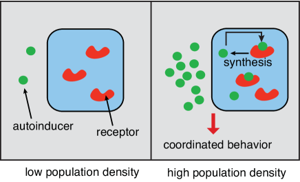
Bacterial quorum sensing Muller13 ; Gou16 ; Iyan21a ; Iyan21b . One of the major applications of model III is bacterial quorum sensing (QS), which is a form of collective chemical sensing and response that depends on population density555A modified version of the PDE-ODE system given by equations (2.2) and (2.4) has been used to model the spatial spread of an airborne disease between localized patches of human populations David20 . The dynamics within a patch is given by an SIR (susceptible-infected-recovered) model, with the rate of infection determined by the concentration of pathogen on the boundary . The field represents the concentration of diffusing pathogen outside the local populations. For simplicity, the movement of people between patches is ignored.. Examples include bioluminescence, biofilm formation, virulence, and antibiotic resistance Waters05 ; Hense15 ; Perez16 ; Papenfort16 ; Muk19 . Bacterial QS involves the exchange of certain signalling molecules called autoinducers between the intracellular and extracellular environments. At low cell densities the concentration of autoinducers within individual cells is too low to trigger a cellular response. However, as the population grows, the concentration of autoinducers passes a threshold, resulting in the activation of various genes including those responsible for synthesising the autoinducers. The resulting positive feedback loop means that all of the cells initiate transcription at approximately the same time, resulting in some form of coordinated behaviour. The basic process at the single-cell level is shown in Fig. 5.
Most models of bacterial QS assume that extracellular diffusion is sufficiently fast so that one can treat the system as a population of identical homogeneous cellular compartments diffusively coupled to a well-mixed extracellular compartment . The corresponding dynamics is given by a system of coupled nonlinear ODEs of the form
| (2.12a) | ||||
| (2.12b) | ||||
where is the uniform extracellular autoinducer concentration, is the autoinducer concentration within the -th cell, and is the volume fraction of the cytosol relative to the extracellular domain. (Note that is related to the cell density.) However, in order to take into account the effects of bulk diffusion, it is necessary to consider the coupled PDE-ODE model given by equations (2.2) and (2.4) with a cytosolic degradation rate, and .
3 Matched asymptotics: steady-state analysis
Consider the steady-state diffusion problem for a constant boundary field (model I):
| (3.1a) | |||
| (3.1b) | |||
| (3.1c) | |||
The corresponding steady-state equations for model II are
| (3.2a) | |||
| (3.2b) | |||
| (3.2c) | |||
| (3.2d) | |||
Finally, the steady-state version of model III is obtained by setting in equation (3.1),with
| (3.3) |
Given the basic assumption that the compartments are small and well-separated, we can use a combination of matched asymptotics and Green’s function methods along the lines of Refs. Ward93 ; Ward93a ; Straube07 ; Gou16 ; Bressloff23a in 2D and Refs. Straube09 ; Cheviakov11 ; Bressloff23b in 3D. More specifically, we construct an inner or local solution valid in an neighbourhood of each compartment, and then match to an outer or global solution that is valid away from each neighbourhood. The general construction is illustrated in Fig. 6. We now give a detailed description of the steps of the analysis, first in 2D and then 3D. In both cases, we develop the asymptotic analysis for model I and then indicate how to extend the analysis models II and III. We also perform the rescalings
| (3.4) |
so that the total flux across the boundary and the rates of insertion and removal within are 666One example where the reactivity is not rescaled is in a conversion-limited model of Ostwald ripening during the liquid-liquid phase separation of biological condensates Lee21 ; Bressloff24b Taking the flux across each droplet boundary to be means that the coarsening of droplets is significantly slowed down, resulting in the coexistence of multiple droplets over relevant biological timescales. The corresponding matched asymptotic analysis has to be modified accordingly.. Finally, without loss of generality, se take . (If then we simply perform the shifts , etc.)
3.1 Asymptotic analysis in 2D
In the 2D case (), the inner solution of equations (3.1) near the -th compartment is constructed by introducing the stretched local variable and setting
| (3.5) |
The inner solution then satisfies (on dropping terms)
| (3.6a) | |||
| (3.6b) | |||
Using polar coordinates with and setting , we have
| (3.7) |
which has the general solution
| (3.8) |
with
| (3.9) |
In order to determine the coefficients we have to match the far-field behaviour of the inner solution with the outer solution. The outer solution is constructed by shrinking each compartment to a single point and imposing a corresponding singularity condition that is obtained by matching with the inner solution. The outer equation is given by
| (3.10) |
for together with the boundary condition . The corresponding singularity conditions are
| (3.11) |
for . A common feature of strongly localised perturbations in 2D domains Ward93 is the appearance of the small parameter
| (3.12) |
In order to eliminate the term in the singularity condition (3.11), we rescale the unknown coefficients by setting . It is well-known that more slowly than . Hence, if one is interested in obtaining accuracy with respect to an expansion, then it is necessary to sum over the logarithmic terms non-perturbatively Ward93 ; Ward93a .
The first step is to introduce the Neumann Green’s function of the modified Helmholtz equation according to777There are very few geometries for which the 2D or 3D Neumann Green’s function of the modified Helmholtz equation is known explicitly, see appendix A.
| (3.13a) | ||||
| (3.13b) | ||||
Note that the 2D Green’s function can be decomposed as
| (3.14) |
where is the non-singular part of the Green’s function. It follows that the solution of equation (3.10) can be written in the form
| (3.15) |
We have unknown coefficients , which are determined by matching the inner and outer solutions:
| (3.16) |
We have set for convenience, with . Let us rewrite equation (3.16) as a matrix equation:
| (3.17) |
where is the identity matrix,
| (3.18) |
and is an matrix with entries
| (3.19) |
Inverting equation (3.17) yields in component form
| (3.20) |
with
| (3.21) |
Note that the solution (3.20) for is a non-perturbative function of the small parameter , which was obtained by matching the inner and outer solutions using Green’s functions along the lines originally developed in Refs. Ward93 ; Ward93a . This effectively sums over the logarithmic terms, which is equivalent to calculating the asymptotic solution for all terms of for any . It is with respect to a corresponding expansion. If one were to Taylor expand equation (3.20) in powers of , then the leading order form of the outer solution would be
| (3.22) |
Finally, note that the asymptotic solution (3.20) still holds in the limit , except that . This corresponds to having the Dirichlet boundary condition for all .
Zero degradation ().
Special care has to be taken when , since the solution of Laplace’s equation in a bounded domain with a reflecting boundary is only defined up to a constant. The corresponding generalised Neumann Green’s function satisfies the equation
| (3.23a) | ||||
| (3.23b) | ||||
for fixed . The additional constant term on the right-hand side of equation (3.23a) is needed in order to ensure that both sides yield zero when integrating with respect to . The condition determines uniquely. Again we can decompose as
| (3.24) |
where is the regular part of the Green’s function . (Some examples of in simple geometries are collected in appendix A.) The analysis of the inner solution is identical to the case . However, the outer solution is now only defined up to a constant such that
| (3.25) |
for and some constant . Since , it follows that
| (3.26) |
In addition, if then
Hence, the outer solution satisfies the steady-state diffusion equation if and only if
| (3.27) |
In order to determine the unknown coefficients, , and , we require linearly independent conditions. One of these is given by equation (3.27) whereas the others are obtained from matching the inner and outer solutions. Proceeding along similar lines to the derivation of equation (3.20) we find that
| (3.28) |
with
| (3.29) |
Imposing the constraint (3.27) on equation (3.28) then determines the unknown constant :
| (3.30) |
Finally, note that expanding equations (3.28) and (3.30) to yields
| (3.31) |
and the outer solution reduces to
| (3.32) |
One important application of the above analysis is determining the coarsening dynamics of 2D Ostwald ripening Kavanagh14 ; Bressloff20a . First, substituting the inner solution (3.8) into equation (2.8) under the adiabatic approximation and setting with gives to leading order
| (3.33) |
Substituting for using equation (2.5) then implies that
| (3.34) |
Hence,
| (3.35) |
where is the harmonic mean of the droplet radii,
| (3.36) |
Including higher-order terms in the asymptotic expansion then yields corrections to this mean field result.
Semi-permeable interface (model II).
The only modification of the inner solution (3.8) and the outer solution (3.15) in the case of a semipermeable interface concerns the calculation of the constants and appearing in the matching condition (3.16). That is, we have to extend the inner solution so that it includes the effects of diffusion within each compartment as determined by equations (3.2). In terms of stretched coordinates, we set
| (3.37) |
The inner solutions then satisfy (on dropping terms)
| (3.38a) | |||
| (3.38b) | |||
| (3.38c) | |||
Using polar coordinates with , the solution can be written as Bressloff23a
| (3.39a) | |||
| (3.39b) | |||
where and is a modified Bessel function of the first kind. The coefficients can be expressed in terms of by imposing equations (3.38c). After some algebra, we find that
| (3.40) |
with
| (3.41) |
It follows that
| (3.42) |
in the matching condition (3.16). Note that in the limit for all we recover model I.
The above model has been used to study the effects of bulk diffusion on synaptic receptor trafficking in somatic inhibitory synapses Bressloff23a . Substituting equation (3.39b) into equation (2.11) then gives the following expression for the steady-state number of receptors in the -th synapse:
| (3.43) |
We have used the Bessel function identity , which implies that
It follows that the synaptic strength as determined by depends on local synaptic parameters such as the rates of endo/exocytosis and , the synaptic diffusivity , and the size of the synapse . However, there is also a heterosynaptic component to the synaptic strength due to the fact that the coefficient depends on all of the other synapses through the matching condition (3.16) Bressloff23a .
Biochemical reaction network (model III).
In compartmental model III the constant is determined from equation (3.3) under the mappings by setting on :
| (3.44) |
We have also set . Using equations (3.8) and (3.9) with , we obtain the nonlinear algebraic system Gou16
| (3.45) |
(Recall from equation (3.20) that the coefficients depend on all the coefficients , .) Since the underlying coupled PDE-ODE system is nonlinear, it follows that there may exist more than one solution of equation (3.45). However, in order to determine the stability of each steady-state solution, one has to linearise the full time-dependent equations and solve a non-trivial eigenvalue problem Gou16 . Linear stability analysis also yields necessary conditions for the occurrence of a Hopf bifurcation, signalling the emergence of collective oscillations. Alternatively, asymptotic methods can be used to reduce the PDE-ODE system to an effective nonlinear ODE system in the fast diffusion regime Gou16 ; Iyan21a ; Iyan21b , providing a more tractable framework for investigating diffusion-mediated synchronisation, see also section 5.
3.2 Asymptotic analysis in 3D
The 3D analysis of equations (3.1) is based on an asymptotic expansion with respect to rather than Straube09 ; Cheviakov11 ; Bressloff23b . The outer solution is expanded as
| (3.46) |
with
| (3.47a) | |||
for . Equations (3.47) are supplemented by singularity conditions as , . The latter are determined by matching to the inner solution. In the inner region around the -th compartment, we again introduce the stretched coordinates and set . Expanding the inner solution as
| (3.48) |
we have
| (3.49a) | |||
| (3.49b) | |||
(Note that for .) Finally, the matching condition is that the near-field behaviour of the outer solution as should agree with the far-field behaviour of the inner solution as , which is expressed as
| (3.50) |
In particular, note that the far-field behaviour of determines the near-field behaviour of so we alternate between the inner and outer solutions during matching.
In order to solve the inner BVP for , we introduce spherical polar coordinates and set :
| (3.51) |
Assuming that the solution decays at infinity, we have
| (3.52) |
(Note that in the limit .) The matching condition (3.50) then implies that satisfies equations (3.47) together with the singularity condition
It follows that the leading order contribution to the outer solution can be written as
| (3.53) |
where is the 3D version of the modified Helmholtz Green’s function defined in equation (3.13). In particular, the 3D Green’s function has the singularity structure
| (3.54) |
Next we match the far-field behaviour of with the non-singular contribution to the near-field behaviour of around . That is, as with
| (3.55) |
It follows that the solution of equation (3.49) for is
| (3.56) |
Hence, satisfies equation (3.47) supplemented by the singularity condition
Following along identical lines to the derivation of , we obtain the result
| (3.57) |
In conclusion, the outer solution takes the form
| (3.58) |
while the inner solution around the -th cluster is
| (3.59) |
Zero degradation ().
As in the case of 2D diffusion, we have to modify the analysis when . In particular, the outer solution has a constant term that has to be determined self-consistently:
| (3.60) |
The leading order contribution to the inner solution now takes the form
| (3.61) |
with defined in (3.52). The subsequent analysis proceeds along identical lines to the previous case. The outer solution becomes
| (3.62) |
while the inner solution around the -th cluster is now
| (3.63) |
Here is the 3D version of the modified Green’s function of equation (3.23), and is given by equation (3.55) after replacing by . The unknown constant is determined by ensuring that the outer solution (3.62) satisfies the steady-state equation . Applying the Laplacian to both sides of equation (3.62) implies that for , we have
It follows that to
| (3.64) |
Equations of the form (3.58) and (3.62) have been used to characterise the spatial decay of intracellular protein gradients under phosphorylation- dephosphorylation Straube09 . Analogous to the 2D case, equation (3.62) has also been used to determine droplet coarsening dynamics in 3D Ostwald ripening. Substituting equation (2.5) into equation (3.64) and taking the limit , we have
| (3.65) |
Moreover, since with , we find that equation (2.8) becomes
| (3.66) |
Hence, at time all droplets satisfying () are growing (shrinking). This means that the critical radius is an increasing function of time so that only a single droplet remains in the limit .
Semi-permeable interface (model II).
Consider the 3D version of the inner BVP (3.38). Introducing the series expansions
| (3.67) |
we have for
| (3.68a) | |||
| (3.68b) | |||
| (3.68c) | |||
For the sake of illustration, we calculate the leading order contribution (), which in spherical polar coordinates is the solution to the BVP
| (3.69a) | |||
| (3.69b) | |||
| (3.69c) | |||
Assuming that vanishes at infinity, we obtain a solution of the form
| (3.70) |
with . Substituting into the boundary conditions (3.69c) gives
| (3.71) |
which can be rearranged to yield the result
| (3.72) |
with defined in (3.52). Note that we recover equation (3.52) with in the fast diffusion limit .
Biochemical reaction network (model III).
The 3D version of equation (3.44) is
| (3.73) |
Using equation (3.59) with , we thus obtain the nonlinear algebraic system
| (3.74) |
The existence of steady-state solutions and the reduction of the PDE-ODE system to a nonlinear ODE system is developed in Ref. Muller13 . However, as far as we are aware, the emergence of collective oscillations via a Hopf bifurcation has not yet been explored in 3D.
4 Relaxation to steady state and the accumulation time
Models I and II are linear diffusion problems and we expect the system to relax to a unique steady-state. In many applications one is also interested in characterizing the relaxation to steady state. A standard approach is to calculate the principal nonzero eigenvalue of the negative Laplacian Ward93 ; Ward93a ; Cheviakov11 . However, this is a global measure of the relaxation process that does not account for possible differences in the relaxation rate at different spatial locations. In addition, it relies on the assumption that the eigenvalues have sufficiently large spectral gaps. Therefore, in this section we use asymptotic methods to calculate the accumulation time for singularly perturbed diffusion problems Bressloff22 ; Bressloff23 .
Following Ref. Bressloff22 , consider the simple motivating example of diffusion along the finite interval, , with a constant flux at the end and a reflecting boundary at . The concentration satisfies the diffusion equation888In the particular application to morphogenesis, represents the extracellular morphogen concentration gradient along the body axis of a developing embryo, while the boundary flux at is generated by local protein synthesis Berez10 ; Berez11 ; Berez11a ; Gordon11 . The constant is an effective degradation rate due to binding of morphogen to cell surface receptors. The spatially varying morphogen concentration drives a corresponding spatial variation in gene expression through some form of concentration thresholding mechanism.This converts a continuously varying morphogen concentration into a discrete spatial pattern of differentiated gene expression across a cell population. One constraint of the model is that the concentration gradient should be established within appropriate developmental time scales.
| (4.1) |
with . If , then the boundary condition at can be neglected and with identified as the space constant for exponential decay. One way to quantify the relaxation to steady state is to consider the eigenfunction expansion
| (4.2) |
where , , are the eigenvalues and eigenfunctions of the linear operator with homogeneous boundary conditions:
| (4.3) |
The eigenfunctions form a complete orthonormal set
| (4.4) |
A straightforward calculation shows that
| (4.5) |
If the positive eigenvalues are well separated, then the relaxation to steady state will be dominated by the term with and constant. (The constants are determined by the initial condition.) Hence, we can identify as the effective relaxation time.
In order to define the corresponding accumulation time for the above 1D problem, let
| (4.6) |
denote the fractional deviation of the concentration from steady state. Assuming that there is no overshooting, i. e. no sign reversal of ), then can be interpreted as the fraction of the steady-state concentration that has accumulated at by time . It follows that is the fraction accumulated in the interval . The accumulation time at position is then defined as Berez10 ; Berez11 ; Gordon11 :
| (4.7) |
In terms of the eigenfunction expansion (4.2),
| (4.8) |
which is non-singular since for all . For the simple diffusion process given by equation (4.1), can be calculated explicitly in the limit and one finds that Berez10
| (4.9) |
Let us now turn to equations (2.2) with (model I) and an initial condition with having compact support on . Suppose that there exists a unique solution of the steady-state equations (3.1). In contrast to the above 1D example, care has to be taken regarding the sign of . If the initial condition , then for all since the boundaries act as source terms. On the other hand, if has sufficient nonzero compact support then the boundaries act as sinks and for all . We will consider the latter example here and thus reverse the sign in the definition of the accumulation time:
| (4.10) |
where we have introduced the Laplace transform . Laplace transforming the higher-dimensional version of equation (4.12) implies that
| (4.11) |
so that the corresponding accumulation time can be written as
| (4.12) |
(In order to calculate the accumulation time for higher-dimensional diffusion in a singularly perturbed domain, it is more convenient to work in Laplace space.) Laplace transforming equations (2.2) with and , we have
| (4.13a) | ||||
| (4.13b) | ||||
| (4.13c) | ||||
Mathematically speaking, these equations are identical in form to the steady-state problem under the mappings , and an effective external input . Hence, the asymptotic methods presented in section 3 can be extended to solve the diffusion problem in Laplace space. (This also holds for model II, but breaks down in the case of model III due to the presence of nonlinear time-dependent terms; extensions of the latter beyond steady-state analysis will be discussed in section 5.) Also note that the steady-state solution could also be recovered using the identity
One subtle feature about working in Laplace space concerns the small- behaviour of the corresponding Green’s function , which is defined by equations (3.13) under the mapping . (The small- behaviour is needed in order to evaluate the accumulation time using equation (4.12).) For , the Green’s function is a nonsingular function of such that . However, in the special case (zero degradation), has a simple pole at such that Bressloff22 ; Bressloff23
| (4.14) |
where satisfies equations (3.23). This causes particular problems in 3D, since we obtain a double series expansion in and that includes terms in powers of . Although such terms can be eliminated by performing partial summations, the details are rather technical Bressloff23 . Therefore, we will restrict the analysis to the case .
4.1 Asymptotic analysis in 2D
Following along identical lines to section 3.1, the inner solution takes the form
| (4.15) |
provided that . (Since we are ultimately interested in the limit , this restriction is not an issue here.) Similarly, the outer solution becomes
| (4.16) |
where
| (4.17) |
Matching the inner and outer solutions yields a system of equations for the unknown coefficients :
| (4.18) |
We thus obtain the matrix solution
| (4.19) |
with
| (4.20) |
and
| (4.21) |
For , the Green’s function is non-singular in the limit . Hence, multiplying the outer solution (4.16) by , differentiating with respect to and taking the limit gives
| (4.22) |
where
| (4.23) |
is the coefficient of the corresponding steady-state solution, and
| (4.24) |
with
| (4.25) |
We have multiplied both sides of equation (4.19) by and differentiated with respect to using the matrix identity
| (4.26) |
for any invertible and differentiable matrix . Combining the various results yields the following general expression for the accumulation time:
| (4.27) | |||||
A general result of this analysis is that the accumulation time diverges as in the case of a nonzero initial condition in the bulk, for which the compartments act as strongly localised sinks. The situation is very different if for all , since the compartments now act as strongly localised sources from which particles diffuse into the bulk. Reversing the sign in the definition of the accumulation time, we have .
4.2 Asymptotic analysis in 3D
We now turn to the aysmptotic analysis of equations (4.13) in 3D. The outer solution can be expanded as
| (4.28) |
with
| (4.29a) | |||
| (4.29b) | |||
for . Equations (4.29) are supplemented by singularity conditions as , . The latter are determined by matching to the inner solution
| (4.30) |
where
| (4.31a) | |||
| (4.31b) | |||
The matching condition is now
| (4.32) |
In order to perform this matching, we need to Taylor expand near the -th compartment and rewrite it in terms of stretched coordinates:
| (4.33) |
It immediately follows that the contribution to the inner solution no longer vanishes at infinity. In particular,
| (4.34) |
The matching condition (4.32) then implies that satisfies equations (4.29) together with the singularity condition
Hence, we have the solution
| (4.35) |
Combining the non-singular near-field behaviour of with equation (4.33) implies that
| (4.36) |
where for , and .
The first term on the right-hand side generates contributions to the inner solution in the form of first-order spherical harmonics, which only affect the outer solution at . In order to show this, we decompose the solution around the -th compartment as with
and
The solution for is then
| (4.37) |
In order to determine , we introduce local spherical polar coordinates such that and , . In spherical polar coordinates we have
| (4.38) | |||
| (4.39) |
Recall that Laplace’s equation in spherical polar coordinates has the general solution
| (4.40) |
where is an associated Legendre polynomial. Imposing the Dirichlet boundary condition and the far-field condition implies that
| (4.41) |
Clearly this leads to a singular term that is .
In summary, we obtain an outer solution of the form
| (4.42) |
Multiplying both sides by , differentiating with respect to and taking the limit gives
| (4.43) |
We conclude that
| (4.44) | |||||
As in the 2D case, is singular in the limit for having nonzero support, but is finite when (after a sign reversal).
5 Asymptotic reduction of a 2D PDE-ODE model to a nonlinear ODE system
In contrast to the linear models I and II , which are based on linear diffusion equations, model III describes a nonlinear coupled PDE-ODE system that can support multiple steady-state solutions. However, only those that are linearly stable will be observable. Moreover, a steady-state solution may undergo a bifurcation due to one or more eigenvalues associated with the linearised system crossing the imaginary axis, resulting in a modified set of unstable and stable steady-state solutions, and possibly the emergence of a limit cycle. The linear stability of the 2D model and conditions for a Hopf bifurcation have been analysed in Ref. Gou16 . Asymptotic methods have also been used to reduce the PDE-ODE system to an effective nonlinear ODE system in the well mixed limit Gou16 ; Iyan21a , and this analysis has subsequently been extended to the regime Iyan21b . The reduced models provided a more tractable mathematical framework for investigating the role of diffusion-mediated coupling on the collective dynamics of compartmental oscillators, at least in the fast diffusion regime. In this section we review the asymptotic reduction of Ref. Iyan21b 999Extending asymptotic and numerical methods to the time domain is an important topic for future work in this area. A recent preprint by Pelz and Ward Pelz24 develops a hybrid asymptotic-numerical theory for studying diffusion-mediated collective oscillations. In particular, these authors extend asymptotic methods for analyzing equations (2.2) and (2.4) to the time-dependent setting without any restrictions on the diffusivity. This leads to a novel integro-differential ODE system that characterizes intracellular dynamics in a memory-dependent bulk-diffusion field. They also introduce a fast time-marching scheme to compute numerical solutions to the integro-differential system over long time intervals..
The main idea is to derive an ODE for the mean bulk concentration
| (5.1) |
which is accurate to and couples to the dynamical variables , . First, integrating equation (2.2a) with and , and using the divergence theorem shows that
| (5.2a) | |||
| where we have taken (assuming that is not too large). Moreover, | |||
| (5.2b) | |||
Assuming , set with . The inner solution around the -th compartment satisfies the equation
| (5.3a) | |||
| (5.3b) | |||
Using polar coordinates with and setting , we have the solution
| (5.4) |
where
| (5.5) |
Substituting the inner solution into equations (5.2) then gives
| (5.6a) | |||
| (5.6b) | |||
It remains to determine the coefficients , by matching the inner solution with the outer solution, which satisfies
| (5.7a) | ||||
| (5.7b) | ||||
| (5.7c) | ||||
Introduce the expansion
| (5.8) |
Substituting into the outer equations shows that Iyan21b
| (5.9a) | |||
| (5.9b) | |||
| (5.9c) | |||
The sum over Dirac delta functions in equation (5.9) ensures that is consistent with equation (5.6) when integrated over . Proceeding as in previous sections, we write
| (5.10) |
where satisfies equations (3.23). Finally, matching the inner and outer solutions using equation (5.9c) gives
| (5.11) |
In summary, as originally shown in Ref. Iyan21b , the PDE-ODE system of model III with bulk diffusivity can be reduced to an ODE system given by equations (5.6) with coefficients determined by the matrix equation (5.11). In order to relate this result to the classical ODE system (2.12a), suppose that all the cells are identical so that and . The solution of equation (5.11) can then be written as
| (5.12) |
and equations (5.6) become
| (5.13a) | |||
| (5.13b) | |||
where . Since in the well-mixed limit , equations (5.13) reduce to the non-spatial model (2.12a) with . However, all information regarding the scaled diffusivity and the spatial configurations of the cells via the dependence of on is lost. The effects of these features on synchrony and oscillatory dynamics of diffusion-mediated quorum sensing are explored in some detail in Ref. Iyan21b by considering the particular example of Sel’kov reaction kinetics. (The latter was originally introduced as a simple model of glycolysis oscillations in yeast cells Selk68 .) Each isolated compartment is assumed to be slightly below the threshold for the onset of oscillations. In the presence of diffusion-mediated cell–cell interactions with , one finds that for a range of parameter values and geometric arrangements of cells, the coupled system can undergo a Hopf bifurcation resulting in collective synchronisation. However, these collective oscillations disappear in the well-mixed limit, indicating the crucial role of bulk diffusion in the emergence of synchrony.
6 Themes and variations
We conclude by discussing some generalisations and open problems arising from the theoretical framework presented in previous sections.
6.1 Non-spherical compartments
As originally shown by Ward and Keller Ward93 ; Ward93a , it is possible to generalise the asymptotic analysis of singularly perturbed diffusion problems to more general compartmental shapes such as ellipsoids by applying classical results from electrostatics. In particular, note that the low-order terms in the expansion of the inner solution around the -th compartment satisfy Laplace’s equation. This is supplemented by a Robin boundary condition on together with some far-field condition. For the sake of illustration, suppose that the Robin boundary condition is replaced by the Dirichlet condition on and as . (Given the solution to Laplace’s equation, one could determine self-consistently by imposing the Robin boundary condition.) We can then write the solution as
| (6.1) |
with satisfying the boundary value problem
| (6.2) |
This is a well-known problem in electrostatics and has the far-field behaviour
| (6.3) |
where is the capacitance and the dipole vector of an equivalent charged conductor with the shape . (Here has the units of length.) Some examples of capacitances for various trap shapes are as follows Cheviakov11 :
One typically finds that low-order terms in the asymptotic expansion for non-spherical compartments can be obtained from the corresponding expressions for the spherical case by replacing the scaled radius with the more general shape capacitance . An analogous result holds for 2D with replaced by the so-called logarithmic capacitance.
6.2 Switching processes
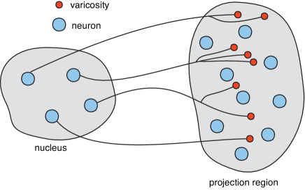
Volume transmission. There is at least one example of a singularly perturbed diffusion problem in cell biology that is not covered by the boundary conditions shown in Fig. 2, namely, volume transmission. The latter refers to a form of neural communication whereby a population of neurons makes non-specific connections to other brain regions Fuxe10 ; Reed23 . That is, rather than forming one-to-one synaptic connections to other neurons, they simply release neurotransmitter into the extracellular space from numerous axon terminals known as varicosities. A number of well-known neurotransmitters participate in volume transmission, including serotonin, dopamine, histamine and acetylcholine. In most cases, the cell bodies are located in brain stem nuclei and their axons project to a distant brain region such as the striatum or cortex, where they release the neurotransmitter, see Fig. 7. Recently, volume transmission has been formulated as an example of diffusion in a singularly perturbed domain in which the boundaries randomly switch between open and closed states Lawley18 ; Lawley20 . That is, each compartment represents a varicosity that acts as a source of neurotransmitter when the source neuron fires and is a sink for neurotransmitter otherwise. The latter is due to the re-uptake of neurotransmitter into the terminals.
The model equations take the form
| (6.4a) | ||||
| (6.4b) | ||||
| (6.4c) | ||||
| (6.4d) | ||||
Here is a constant flux of neurotransmitter into the extracellular space when the corresponding source neuron is firing. Note that the volume is the extracellular space that includes the varicosities but excludes the target cells. Equations (6.4) are an example of a diffusion process in a randomly switching environment Bressloff15a ; Bressloff15b . One way to analyze such a system is to take expectations with respect to the random switching process, conditioned on the current state of the environment. For the sake of illustration, suppose that all the source neurons fire synchronously and that switching between the global quiescent and firing states is described by a two-state Markov chain with transition rates :
| (6.5) |
(If each varicosity switched independently then we would have a Markov chain of size , where is the number of varicosities.) Let denote the current state of the source neurons, and introduce the conditional expectations
| (6.6) |
It can then be shown that evolves according to the equations
| (6.7a) | ||||
| (6.7b) | ||||
| (6.7c) | ||||
The matrix generator of the Markov chain is
| (6.8) |
The steady-state can then be obtained by performing two successive asymptotic expansions based on model I. First, suppose that we replace the inhomogeneous Neumann boundary condition for on by the Dirichlet boundary condition for some unknown constant . Summing the steady-state version of equations (6.7) with respect to and setting gives
| (6.9a) | ||||
| (6.9b) | ||||
This is equivalent to equations (3.1) for model I in the limits and . Solving the latter equation along the lines outlined in section 3, we then set and in the steady-state version of equations (6.7):
| (6.10a) | |||
| (6.10b) | |||
Equations (6.10) yield another version of model I, with and an external input , which can also be solved using the methods of section 3. The resulting solution depends on the unknown constants , which are finally determined by imposing the original Neumann boundary condition for Lawley20 . (An analogous pair of BVPs arises in the analysis of narrow escape through a stochastically-gated boundary Bressloff15b .)
One general result that emerges from the singular-perturbation theory is that the leading order term in the asymptotic expansion of the extracellular concentration is a constant that is independent of the number and location of the varicosities, correlations in neural firings, and the size and geometry of the extracellular space Lawley20 . These features do appear in the next leading order term, which may still be space-independent under mild assumptions.
Active phase separation. Another example of a singularly perturbed diffusion problem with switching is a model for the active suppression of Oswald ripening during the formation of multiple biological condensates. In this model, solute molecules randomly and independently switch between two conformational states, one phase separating () and the other soluble Wurtz18 ; Lee19 . It is assumed that switching between the states and occurs according to the chemical reactions
where and are concentration-independent reaction rates. The latter reflects the non-equilibrium nature of the chemical reactions, in which detailed balance does not hold due to the phosphorylating action of ATP, say. Let , , denote the concentration of solute molecules in state . The steady-state diffusion equations take the form Bressloff20a ; Bressloff20b
| (6.11a) | ||||
| (6.11b) | ||||
| supplemented by the boundary conditions | ||||
| (6.11c) | ||||
The unknown constants are determined by solving a second pair of diffusion equations within each droplet and imposing flux continuity of the soluble phase across :
| (6.12a) | ||||
| (6.12b) | ||||
| supplemented by the boundary conditions | ||||
| (6.12c) | ||||
The flux continuity conditions are
| (6.13) |
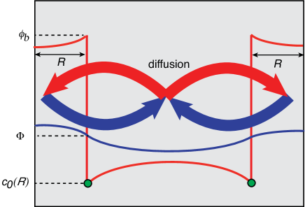
The combination of non-equilibrium chemical reactions, phase separation and diffusion can lead to a stationary state consisting of multiple high density droplets that is maintained by circulating fluxes of and molecules. The basic mechanism is illustrated in Fig. 8 for a pair of droplets. As in classical Ostwald ripening, dynamical equations for the droplet radii can be derived using mean field theory under an adiabatic approximation. The resulting equations support a stable fixed point that represents a multi-droplet solution Wurtz18 ; Lee19 . Singular perturbation theory has subsequently been used to investigate corrections to mean field theory, which take into account finite-size effects associated with the boundary of the domain and the positions of the droplets Bressloff20a .
Switching boundaries versus switching particles. One significant difference between the model of volume transmission and the model of active phase separation is that in the former case the boundaries physically switch, whereas in the latter case it is the particles that independently switch states. These two distinct scenarios are. illustrated in Fig. 9. For a sufficiently large number of solute molecules, the diffusion equations of active phase separation are deterministic. On the other hand, all particles move in the same randomly switching environment during volume transmission, which means that equations (6.4) are stochastic. In other words is a stochastic field, and equations (6.7) are first-moment equations. It is also possible to derive singularly-perturbed diffusion equations for the second-order moments etc. From these it can be shown that the randomly switching environment induces statistical correlations between the particles even though they are not interacting. For example,
| (6.14) |
One direction for future exploration would be to apply singular perturbation theory to these higher-order moment equations.
6.3 The Kuramoto model
The original non-spatial model (2.12a) has motivated a number of theoretical studies of simplified oscillator models coupled via quorum sensing Schwab12 ; Schwab12a ; Sharma16 ; Verma19 . In particular, following Ref. Schwab12 ; Schwab12a , suppose that each oscillator is just beyond a Hopf bifurcation point so that its state at time can be represented by a complex amplitude , 101010This contrasts with the regime considered in Ref. Iyan21b , where each isolated oscillator is below the Hopf bifurcation threshold.. It follows that the state of the environment can be represented by a complex variable , which diffusively couples to each . Let be the natural frequency of the -th oscillator. The frequencies are randomly drawn from a distribution , which is taken to be an even function about a mean frequency . Finally, moving to a rotating frame with frequency , the dynamics of the system can be represented by the equations
| (6.15a) | ||||
| (6.15b) | ||||
In the rotating frame the frequencies are drawn from an even distribution with zero mean. Suppose that equation (6.15a) is rewritten in polar coordinates with and :
| (6.16a) | ||||
| (6.16b) | ||||
As a further simplification, consider the large limit with in steady-state for all . This allows us to effectively eliminate the dynamics of the amplitudes . After performing the rescalings and , equations (6.15) reduce to Schwab12a
| (6.17a) | ||||
| (6.17b) | ||||
Equations (6.17) are a modified version of the classical Kuramoto model Kuramoto84 ; Strogatz00 , in which is identified with the state of an external medium rather than the first circular moment of the oscillators. The latter is defined according to
| (6.18) |
Here is equal to the average phase and is a measure of the degree of phase-coherence; a completely incoherent state corresponds to the case , whereas a completely synchronised state satisfies .
The collective behaviour of the globally-coupled model given by equations (6.17) can be investigated in the thermodynamic limit by considering a continuum mean field model Schwab12a . Let denote the density of oscillators with frequency that have a phase in the interval at time with the normalization
| (6.19) |
Since the total number of oscillators with frequency is fixed, we have the continuity or Liouville equation
| (6.20a) | |||
| and | |||
| (6.20b) | |||
where
| (6.21) |
The modified ODE system (5.13), which takes into account the effects of finite diffusion in the bulk, suggests a generalisation of equations (6.17) of the following form:
| (6.22a) | ||||
| (6.22b) | ||||
It would be interesting to explore how the presence of the matrix affects synchronization and clustering of the original model for finite . However, in contrast to equations (6.17), taking the thermodynamic limit of equations (6.22) doesn’t make sense, since the reduction of the PDE-ODE system to the ODE system (5.13) assumes that the compartments are well-separated. This assumption would break down in the limit , at least in a bounded domain .
Acknowledgements
I would like to thank Michael Ward (University of British Columbia) for many stimulating discussions regarding the asymptotic methods that he and his collaborators pioneered.
Appendix A: Neumann Green’s functions in simple geometries
One of the crucial features of the asymptotic expansions presented in this review is the involvement of the Neumann Green’s function of the modified Helmholtz equation and the generalised Neumann Green’s function of Laplace’s equation, see equations (3.13) and (3.23), respectively. Explicit expressions for these Green’s functions and their regular parts are only known for a small set of geometries, particularly in the case of the modified Helmholtz equation. In this appendix we collect some of the known results.
(a) Laplace’s equation on the disc. Let be the unit circle centred at the origin. The 2D Neumann Green’s function is given by
| (A.1) |
with the regular part obtained by dropping the first logarithmic term.
(b) Laplace’s equation the sphere. Let be the sphere of radius centred about the origin. The 3D Neumann Green’s function takes the form Cheviakov11
| (A.2) |
where the constant is chosen so that , and
It can be shown that is independent of .
(c) Laplace’s equation in a rectangular domain. Let be a rectangular domain . The 2D Neumann Green’s function has the logarithmic expansion Bressloff08 ; Pillay10
| (A.3) |
where
and
| (A.4) |
Assuming that , we have the approximation
The only singularity exhibited by equation (A.3) occurs when , , in which case and the term diverges. Writing
where the first term on the right hand side is singular and the second is regular, we find that
| (A.5) |
where is the regular part of the Green’s function given by
| (A.6) |
(d) Modified Helmholtz equation in a sphere Grebenkov20 .
| (A.7) |
with
| (A.8) |
Here is a Legendre polynomial, , and are modified spherical Bessel functions,
| (A.9) |
In order to simplify the analysis, we will assume that the initial position is at the centre of the sphere. Using the identities
| (A.10) |
we see that
| (A.11) |
Similarly,
| (A.12) |
Further useful identities are
| (A.13) |
The 3D Neumann Green’s function for Laplace’s equation in the sphere can also be written down explicitly so that Cheviakov11
| (A.14) | ||||
for , where . It also follows that
| (A.15) |
and
| (A.16) |
References
- (1)
- (2) Alikakos ND, Fusco G and Karali G (2004) Ostwald ripening in two dimensions – the rigorous derivation of the equations from the Mullins-Sekerka dynamics. J. Diff. Eqs. 205: 1-49.
- (3) Baillou R and Ranft J (2023) Non-equilibrium cluster-cluster aggregation in the presence of anchoring sites. arXiv:2308.15162v1.
- (4) Berezhkovskii AM, Sample C and Shvartsman S Y (2010) How long does it take to establish a morphogen gradient? Biophys. J. 99 L59-L61
- (5) Berezhkovskii AM, Sample C and Shvartsman S (2011) Formation of morphogen gradients: local accumulation time. Phys Rev E 83: 051906
- (6) Berezhkovskii AM and Shvartsman S (2011) Physical interpretation of mean local accumulation time of morphogen gradient formation. J. Chem. Phys. 135: 154115
- (7) Berry J, Brangwynne CP and Haataja HP (2018) Physical principles of intracellular organization via active and passive phase transitions. Rep. Prog. Phys. 81: 046601.
- (8) Biederer T, Kaeser PS and Blanpied TA (2017) Transcellular nanoalignment of synaptic function. Neuron 96: 680-696.
- (9) Borgdorff AJ and Choquet D (2002) Regulation of AMPA receptor lateral movements. Nature 417: 649-653.
- (10) Brangwynne CP, Tompa P and Pappu RV (2015) Polymer physics of intracellular phase transitions. Nature Phys. 11: 899-904.
- (11) Bressloff PC and Earnshaw BA (2007) Diffusion-trapping model of receptor trafficking in dendrites. Phys. Rev. E 75: 041916.
- (12) Bressloff PC, Earnshaw BA and Ward MJ (2008) Diffusion of protein receptors on a cylindrical dendritic membrane with partially absorbing targets. SIAM J. Appl. Math. 68: 1223-1246.
- (13) Bressloff PC and Lawley SD (2015) Moment equations for a piecewise deterministic PDE. J. Phys. A 48: 105001
- (14) Bressloff PC and Lawley SD (2015) Escape from subcellular domains with randomly switching boundaries. Multiscale Model. Simul. 13: 1420-1455
- (15) Bressloff PC, Lawley SD and Murphy P (2019) Protein concentration gradients and switching diffusions Phys. Rev. E 99: 032409
- (16) Bressloff PC (2020) Active suppression of Ostwald ripening: Beyond mean field theory. Phys. Rev. E 101: 042804.
- (17) Bressloff PC (2020) Two-dimensional Ostwald ripening in a concentration gradient. J. Phys. A 53: 365002.
- (18) Bressloff PC (2021) Asymptotic analysis of extended two-dimensional narrow capture problems. Proc. Roy. Soc. A. 477: 20200771.
- (19) Bressloff PC (2021) Asymptotic analysis of target fluxes in the three-dimensional narrow capture problem. Multiscale Model. Simul. 19: 612-632
- (20) Bressloff PC (2022) Accumulation time of diffusion in a 2D singularly perturbed domain. Proc. Roy. Soc A 478: 20210847.
- (21) Bressloff PC (2023) Accumulation time of diffusion in a 3D singularly perturbed domain. SIAM J. Appl. Math. 83:862-881.
- (22) Bressloff PC (2023) 2D interfacial diffusion model of inhibitory synaptic receptor dynamics. Proc. Roy. Soc. A 479:2022.0831.
- (23) Bressloff PC (2023) The 3D narrow capture problem for traps with semipermeable interfaces. Multiscale Modeling and Simulation 21 (2023).
- (24) Bressloff PC (2024) Asymptotic analysis of particle cluster formation in the presence of anchoring sites. Eur. J. Phys. E 47:30
- (25) Bressloff PC. (2024). Asymptotic analysis of conversion-limited phase separation. Proc. Roy. Soc. A 480: 2023.0725.
- (26) Brown GC and Kholodenko BN (1999) Spatial gradients of cellular phospho-proteins. FEBS Lett. 457: 452-454.
- (27) Chapdelaine T, Hakim V, Triller A, Ranft J and Specht CG (2021) Reciprocal stabilization of glycine receptors and gephyrin scaffold proteins at inhibitory synapses. Biophys. J. 120: 805-817.
- (28) Chevalier C, Benichou O, Meyer B and Voituriez R (2011) First-passage quantities of Brownian motion in a bounded domain with multiple targets: a unified approach. J. Phys. A 44: 025002.
- (29) Cheviakov AF and Ward MJ (2011) Optimizing the principal eigenvalue of the Laplacian in a sphere with interior targets. Math. Comp. Modeling 53 042118.
- (30) Choquet D and Triller A (2003) The role of receptor diffusion in the organization of the postsynaptic membrane. Nat. Rev. Neurosci. 4: 251-265.
- (31) Choquet D and Triller A (2013) The dynamic synapse. Neuron 80: 691-703.
- (32) Choquet D (2018) Linking nanoscale dynamics of AMPA receptor organization to plasticity of excitatory synapses and learning J. Neurosci. 38: 9318-9329.
- (33) Coombs D, Straube R and Ward MJ (2009) Diffusion on a sphere with localized traps: Mean first passage time, eigenvalue asymptotics, and Fekete points. SIAM J. Appl. Math. 70: 302-332.
- (34) Delgado MI, Ward M and Coombs D (2015) Conditional mean first passage times to small traps in a 3-D domain with a sticky boundary: Applications to T cell searching behavior in lymph nodes. Multiscale Model. Simul. 13: 1224-1258.
- (35) Cruikshank A, Nijhout HF, Best J and Reed M (2023) Dynamical questions in volume transmission. J. Biol. Dyn. 17: 2269886.
- (36) Czondora K, Mondina M, Garciaa M, Heinec M, Frischknechtc R, Choquet D, Sibaritaa JB and Thoumine OR (2012) A unified quantitative model of AMPA receptor trafficking at synapses. Proc. Nat. Acad. Sci. USA 109: 3522-3527.
- (37) Dahan M, Levi S, Luccardini C, Rostaing P, Riveau B and Triller A (2003) Diffusion dynamics of glycine receptors revealed by single-quantum dot tracking. Science 302: 442-445.
- (38) David JF, Iyaniwura SA, Ward MJ and Brauer F (2020) novel approach to modelling the spatial spread of airborne diseases: an epidemic model with indirect transmission. Math. Bio. Eng. 17: 3294-3328.
- (39) Doi, M 2013 Soft Matter Physics. Oxford University Press, Oxford.
- (40) Earnshaw BA and Bressloff PC (2006) A biophysical model of AMPA receptor trafficking and its regulation during LTP/LTD. J. Neurosci. 26: 12362-12373.
- (41) Earnshaw BA and Bressloff PC (2008) Modeling the role of lateral membrane diffusion on AMPA receptor trafficking along a spiny dendrite. J. Comput. Neurosci. 25: 366-389
- (42) Feric M and Brangwynne CP (2013) A nuclear F-actin scaffold stabilizes ribonucleoprotein droplets against gravity in large cells. Nat. Cell Biol. 15 1253-1259.
- (43) Folkmann. AW, Putnam A, Lee CF and Seydoux G (2021) Regulation of biomolecular condensates by interfacial protein clusters. Science 373: 1218-1224.
- (44) Foret L (2012) Aggregation on a membrane of particles undergoing active exchange with a reservoir. Eur. Phys. J E 35: 12.
- (45) Fuxe K, Dahlstrom AB, Jonsson G, Marcellino D, Guescini M, Dam M, Manger P and Agnati L (2010) The discovery of central monoamine gave volume transmission to the wired brain. Prog.Neurobiol. 90: 82–-00.
- (46) Gordon P, Sample C, Berezhkovskii AM, Muratov CB and Shvartsman S (2011) Local kinetics of morphogen gradients. Proc Natl Acad Sci. 108: 6157-6162
- (47) Gou J and Ward MJ (2016) Asymptotic analysis of a 2-D Model of dynamically active compartments coupled by bulk diffusion. J. Nonlinear Science. 26: 979-1029.
- (48) Grebenkov DS (2020) Diffusion toward non-overlapping partially reactive spherical traps: Fresh insights onto classic problems. J. Chem. Phys. 152: 244108.
- (49) Groc L, Heine M, Cogent L, Brickley K, Stephenson FA, Lounis B and Choquet D (2004) Differential activity-dependent regulation of the lateral mobilities of AMPA and NMDA receptors. Nat. Neurosci. 7: 695-696.
- (50) Hakim V and Ranft J (2020) Lifetime of a structure evolving by cluster aggregation and particle loss, and application to postsynaptic scaffold domains. Phys. Rev. E. 101 012411.
- (51) Haselwandter CA, Calamai M, Kardar M, Triller A and da Silveira RA (2011) Formation and stability of synaptic receptor domains. Phys Rev Lett 106: 238104.
- (52) Haselwandter CA, Calamai M, Kardar M, Triller A and da Silveira RA (2015) Self-assembly and plasticity of synaptic domains through a reaction-diffusion mechanism. Phys. Rev. E 92: 032705.
- (53) Hense BA and Schuster M (2015) Core principles of bacterial autoinducer systems. Microbiol Mol Biol Rev 79: 153-169.
- (54) Holcman D and Triller A (2006) Modeling synaptic dynamics driven by receptor lateral diffusion. Biophys. J. 91: 2405-2415.
- (55) Howard M (2012) How to build a robust intracellular concentration gradient. Trends Cell Biol. 22: 311-317.
- (56) Hyman AA, Weber CA and Jûlicher F (2014) Liquid-liquid phase separation in biology. Annu. Rev. Cell Dev. Biol. 30: 39-58.
- (57) Iyaniwura S and Ward MJ (2021) Localized signaling compartments in 2-D coupled by a bulk diffusion field: Quorum sensing and synchronous oscillations in the well-mixed limit. Europ. J. Appl. Math., 32(5):1001-1031.
- (58) Iyaniwura S and Ward MJ (2021) Synchrony and oscillatory dynamics for a 2-D PDE-ODE model of diffusion-mediated communication between small signaling compartments. SIAM J. Appl. Dyn. Sys., 20(1):438-499.
- (59) Kavanagh E (2014) Interface motion in the Ostwald ripening and chemotaxis systems. Master Thesis, University of British Columbia.
- (60) Keener JP and Sneyd J (2009) Mathematical Physiology I: Cellular Physiology. 2nd edn. Springer, New York.
- (61) Kholodenko BN (2009) Spatially distributed cell signalling. FEBS Letters 583: 4006-4012.
- (62) Kuramoto Y (1984) Chemical Oscillations, Waves, and Turbulence Springer..
- (63) Kurella V, Tzou JC, Coombs D and Ward MJ (2015) Asymptotic analysis of first passage time problems inspired by ecology. Bull Math Biol. 77: 83-125.
- (64) Kusumi A, Nakada C, Ritchie K, Murase K, Suzuki K, Murakoshi H, Kasai RS, Kondo J and Fujiwara T (2005) Paradigm shift of the plasma membrane concept from the two-dimensional continuum fluid to the partitioned fluid: high-speed single-molecule tracking of membrane molecules Annu. Rev. Biophys. Biomol. Struct. 34: 351
- (65) Lawley SD (2018) A probabilistic analysis of volume transmission in the brain. SIAM J. Appl. Math. 78: 942–962.
- (66) Lawley SD and Shankar V (2020) Asymptotic and numerical analysis of a stochastic PDE model of volume transmission. Multiscale Model. Simul. Math. 18: 887-915..
- (67) Lee CF and Wurtz JD (2019) Novel physics arising from phase transitions in biology. J. Phys. D 52: 023001.
- (68) Lee CF (2021) Scaling law and universal drop size distribution of coarsening in conversion-limited phase separation Phys. Rev. Res. 3: 043081
- (69) Levy C and Iron D (2011) Model of cell signal transduction in a three-dimensional domain. J Math Biol 63:831-854.
- (70) Levy C and Iron D (2013) Dynamics and stability of a three-dimensional model of cell signal transduction J. Math. Biol. 67:1691-1728.
- (71) Lifshitz IM and Slyozov VV (1961) The kinetics of precipitation from supersaturated solid solutions. J. Phys. Chem. Solids. 19: 35-50.
- (72) Lindsay AE, Spoonmore RT and Tzou JC (2016) Hybrid asymptotic-numerical approach for estimating first-passage-time densities of the two-dimensional narrow capture problem Phys. Rev. E 94: 042418.
- (73) Lindsay AE, Bernoff AJ and Ward MJ (2017) First passage statistics for the capture of a Brownian particle by a structured spherical target with multiple surface targets Multiscale Model. Simul. 15: 74-109.
- (74) MacGillavry HD, Kerr JM and Blanpied TA (2011) Lateral organization of the postsynaptic density. Mol. Cell. Neurosci. 48: 321-331.
- (75) Maynard SA, Ranft J and Triller A (2023) Quantifying postsynaptic receptor dynamics: insights into synaptic function Nat. Rev. Neurosci. 24: 4-22.
- (76) Meier J, Vannier C, Serge A, Triller A and Choquet D (2001) Fast and reversible trapping of surface glycine receptors by gephyrin. Nature Neurosci. 4: 253-260.
- (77) Meyers J, Craig J and Odde DJ (2006) Potential for control of signaling pathways via cell size and shape. Curr. Biol. 16: 1685-1693.
- (78) Mittag T and Pappu RV (2022) A conceptual framework for understanding phase separation and addressing open questions and challenges. Molecular Cell 82: 2201-2214.
- (79) Mukherjee S and Bassler BL (2019) Bacterial quorum sensing in complex and dynamically changing environments. Nat. Rev. Microbiology 17: 371-382
- (80) Muller J and Uecker H (2013) Approximating the dynamics of communicating cells in a diffusive medium by ODEs - homogenization with localization. J. Math. Biol. 67: 1023-1065.
- (81) Munoz-Garcia J and Kholodenko BN (2010) Signaling and control from a systems perspective. Biochem. Soc. Trans. 38:1235-1241.
- (82) Papenfort K and Bassler BL (2016) Quorum sensing signal-response systems in Gram-negative bacteria. Nat. Rev. Microbiol. 14: 577-588.
- (83) Pelz M and Ward MJ (2024) Synchronized memory-dependent intracellular oscillations for a cell-bulk ODE-PDE model in . Preprint.
- (84) Pérez-Velázquez J, Gölgeli M and García-Contreras R (2016) Mathematical modelling of bacterial quorum sensing: A review. Bulletin of Mathematical Biology, 78: 1585-1639.
- (85) Pillay S, Ward MJ, Peirce A and Kolokolnikov T (2010) An asymptotic analysis of the mean first passage time for narrow escape problems: Part I: Two-dimensional domains. SIAM Multiscale Model. Sim. 8: 803-835.
- (86) Quang BAT, Mani M, Markova O, Lecuit T and Lenne PF (2013) Principles of E-cadherin supramolecular organization in vivo. Current Biology 23:2197-2207.
- (87) Ranft J, Almeida LG, Rodriguez PC, Triller A and Hakim V (2017) An aggregation-removal model for the formation and size determination of postsynaptic scaffold domains, PLoS Computational Biology 13: e1005516.
- (88) Rautu SA, Rowlands G and Turner MS (2018) Europhysics Letters 121: 58004.
- (89) Rosowsk KA, Sai T, Vidal-Henriquez E, Zwicker D, Style RW and Dufresne ER (2020) Elastic ripening and inhibition of liquid-liquid phase separation, Nat. Phys. 16: 422.
- (90) Schumm RD and Bressloff PC (2022) Local accumulation times in a diffusion-trapping model of synaptic receptor dynamics. Phys. Rev. E 105: 064407.
- (91) Schwab DJ, Baetica A and Mehta P (2012) Dynamical quorum-sensing in oscillators coupled through an external medium. Physica D 241: 1782-1788.
- (92) Schwab D, Plunk GG and Mehta P (2012) Kuramoto model with coupling through an external medium. Chaos 22: 043139.
- (93) Sekimoto K and Triller A (2009) Compatibility between itinerant synaptic receptors and stable postsynaptic structure. Phys. Rev. E 79: 031905.
- (94) Sel’kov EE (1968) Self-oscillations in glycolysis 1. A simple kinetic model. European J. Biochem. 4, 79-86.
- (95) Seydoux G (2018) The P Granules of C. elegans: A Genetic Model for the Study of RNA-Protein Condensates. J. Mol. Biol. 430 4702-4710.
- (96) Sharma PR, Kamal NK, Verma UK., Suresh K, Thamilmaran K and Shrimali MD (2016) Suppression and revival of oscillation in indirectly coupled limit cycle oscillators. Phys. Lett. A 380: 3178-3184.
- (97) Straube R, Ward MJ and Falcke M (2007) Reaction rate of small diffusing molecules on a cylindrical membrane. J. Stat. Phys. 129: 377-405.
- (98) Straube R and Ward MJ (2009) An asymptotic analysis of intracellular signaling gradients arising from multiple small compartments, SIAM J.Appl. Math. 70: 248-269.
- (99) Strogatz SH (2000) From Kuramoto to Crawford: Exploring the onset of synchronization in populations of coupled oscillators. Physica D 143: 1-20.
- (100) Style RW, Sai T, Fanelli N, Ijavi M, Smith-Mannschott K, Xu Q, Wilen LA and Dufresne ER (2018) Liquid-liquid phase separation in an elastic network Phys. Rev. X 8: 011028.
- (101) Turner MS, Sens P and Socci ND (2005) Phys. Rev. Lett. 95: 168301.
- (102) Verma UK, Chaurasia SS and Sinha S (2019) Explosive death in nonlinear oscillators coupled by quorum sensing. Phys. Rev. E 100: 032203.
- (103) Wagner C (1961) Theorie der Alterung von Niederschlägen durch Umlösen. Z. Elektrochemie 65: 581-594.
- (104) Ward MJ and Keller JB (1993) Strong localized perturbations of eigenvalue problems. SIAM J Appl Math 53: 770-798.
- (105) Ward MJ, Henshaw WD and Keller JB (1993) Summing logarithmic expansions for singularly perturbed eigenvalue problems. SIAM J. Appl. Math. 53: 799-828.
- (106) Waters CM and Basser BL (2005) Quorum sensing: Cell-to-cell communication in bacteria. Annu. Rev. Cell Dev. Biol. 21: 319-346.
- (107) Weber CA, Zwicker. D, Jülicher F and Lee CF (2019) Physics of active emulsions. Rep. Prog. Phys. 82 064601.
- (108) Wurtz JD and Lee CF (2018) Chemical-reaction-controlled phase separated drops: formation, size selection and coarsening. Phys. Rev. Lett. 120: 078102.
- (109) Zwicker D, Hyman AA and Jülicher F (2015) Suppression of Ostwald ripening in active emulsions. Phys. Rev. E 92: 012317.
- (110)