Multi-Bit Mechanism: A Novel Information Transmission Paradigm for Spiking Neural Networks
Abstract
Since proposed, spiking neural networks (SNNs) gain recognition for their high performance, low power consumption and enhanced biological interpretability. However, while bringing these advantages, the binary nature of spikes also leads to considerable information loss in SNNs, ultimately causing performance degradation. We claim that the limited expressiveness of current binary spikes, resulting in substantial information loss, is the fundamental issue behind these challenges. To alleviate this, our research introduces a multi-bit information transmission mechanism for SNNs. This mechanism expands the output of spiking neurons from the original single bit to multiple bits, enhancing the expressiveness of the spikes and reducing information loss during the forward process, while still maintaining the low energy consumption advantage of SNNs. For SNNs, this represents a new paradigm of information transmission. Moreover, to further utilize the limited spikes, we extract effective signals from the previous layer to re-stimulate the neurons, thus encouraging full spikes emission across various bit levels. We conducted extensive experiments with our proposed method using both direct training method and ANN-SNN conversion method, and the results show consistent performance improvements.
1 Introduction
In recent years, deep learning represented by artificial neural networks (ANNs) has been widely applied in many downstream tasks such as computer vision krizhevsky2012imagenet and game playing silver2016mastering , etc. However, these achievements are mostly built upon high computational budgets, which limits the application of ANNs on edge computing scenarios.
As an alternative, spiking neural networks (SNNs) are proposed. SNNs transmit signals using discrete spikes with temporal characteristics, which is close to the information transmission mechanism of biological neurons, thus being regarded as the third generation of neural networks maass1997networks . Moreover, the sparse nature of the spikes makes the feature matrix sparse, reducing computational load, while their binary characteristics which transforms the multiply-and-accumulate (MAC) operations calculations into accumulate (AC) operations roy2019towards , simplifying the computation. All these, endows SNNs with high performance and low power consumption characteristics diehl2015unsupervised .
However, current SNNs also face challenges. Firstly, the forward process involves the conversion from full-precision membrane potentials to binary spikes, leading to significant information loss. Secondly, the network structures of existing SNNs mostly consist of simple modules where information is transmitted layer by layer, greatly reducing the network’s expressive power.
We claim that the roots of these two problems lie in the characteristics of the neuron structure and network architecture of SNNs, respectively. On one hand, in terms of neuron structure, existing SNNs, like ANNs, typically assume that there is only one synaptic connection between adjacent neurons. However, in biological neural networks, adjacent neurons often have multiple synapses. This may not be crucial for ANNs since they can transmit full-precision real values through a single synapse. But for SNNs, the presence of multiple synapses implies the possibility of transmitting multi-bit signals, which evidently helps to improve the precision of information transmission. Unfortunately, current SNNs simply adopt the single synapse setting like ANNs and thus lose the potential to transmit higher precision data. On the other hand, in terms of network architecture, the information flow in current SNNs is simply transmitted layer by layer. Such mechanism lacks the cross-layer information exchange existing in the biological neural networks, leading to the degenerated expressive power of SNNs. According to thomson2003interlaminar , projections from layer 3 to layer 5 exist in the adult mammalian neocortex.
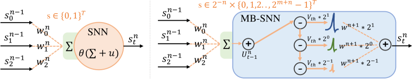
Based on the above considerations, we propose a multi-bit information transmission mechanism as shown in Fig.1 that expands the output of neurons from one bit to multiple bits without introducing extra parameters. This method significantly reduces information loss during the forward process of the network. Additionally, we simulate interlaminar connections. On one hand, this structure enriches the network’s topological connections, enhancing the network’s expressive power. On the other hand, through Efficient Channel Attention (ECA) wang2020eca , this structure extracts effective information from the previous layer of the network to stimulate the current neuron again, further compensating for the lost information. Our contributions are as follows:
-
•
We propose a multi-bit information transmission mechanism. This mechanism expands the output of spiking neurons from single bit to multiple bits. While preserving the low-energy advantages of SNNs, it significantly reduces information loss during the forward process. For SNNs, this represents a new paradigm of information transmission.
-
•
We propose interlaminar connections. This approach further reduces information loss and enhances the network’s expressive capability. Additionally, the sufficient retention of information makes the neurons more active, allowing the multi-bit mechanism to better realize its power.
-
•
We conducted extensive experiments. The results show that whether it is static datasets or neuromorphic datasets; whether it is direct training or ANN-SNN conversion training, our theory consistently demonstrated improvements in the experimental results. It is worth mentioning that even at ultra-low time steps, our method remains highly competitive compared to other methods.
2 Related work
2.1 Training method of SNNs
The training algorithms for SNNs can be categorized into unsupervised and supervised learning algorithms. Unsupervised learning algorithms are mostly bio-inspired, and the most commonly used one is the STDP (Spike-Timing-Dependent Plasticity) algorithm song2000competitive based on synaptic plasticity mechanisms hebb2005organization . These algorithms offer better biological interpretability, but their performance is generally less effective compared to supervised learning algorithms liu2021sstdp .As for supervised learning, due to the non-differentiable nature of spikes, the supervised learning methods for SNNs differ significantly from those for ANNs. Currently, there are two training methods: one is direct training wu2018spatio ; yao2023attention ; wang2022ltmd ; zuo2020spiking ; zuo2022multi , which introduces a differentiable function to approximate the heaviside function. The derivative of this function is used to replace the derivative of the heaviside function at the corresponding position for backpropagation, hence it is also known as the gradient surrogate method. The other method is ANN-SNN conversion bu2023optimal ; liu2022spikeconverter ; kim2020spiking , which first trains an ANN, then replaces the network’s activation function with spiking neurons, allowing the activation values of ANNs to be mapped to the firing rates of spiking neurons and continue to propagate in the network.
2.2 Quantization loss
Previous researchers zheng2021going have proposed and demonstrated that the membrane potential follows a normal distribution with a mean of 0. The occurrences of membrane potential exceeding the threshold are rare in the distribution, leading to a low firing rate of neurons as shown in Fig.3(a), which endows the spike with sparse characteristics. The sparse nature is the source of high performance and low power consumption in SNNs, but it also causes a significant quantization loss, hindering the development of deeper networks. To reduce quantization loss, many researchers have made efforts.
Some attempt to adjust the distribution of the membrane potential to alter the firing rate. zheng2021going indirectly adjust the distribution of membrane potential by adjusting the variance of the input , ensuring that the firing rate remains at a reasonable level. guo2022loss calculates the mutual information between the membrane potential and spikes to conclude that the maximum information content of spikes occurs when the firing rate is 0.5.
Others try to expand spikes into multi-valued ones to enhance the information content of the spikes. feng2022multi packages k LIF neurons with different thresholds into a single MLF unit, where neurons within the unit share inputs and their outputs are summed, resulting in a spike value range of , which increases the diversity of the output spikes. zhao2022backeisnn proposes an inhibitory type of spike, expanding the range of spike values to . Similarly, guo2024ternary also introduces ternary spikes, using as a scaling coefficient to set the spike values to .
3 Method
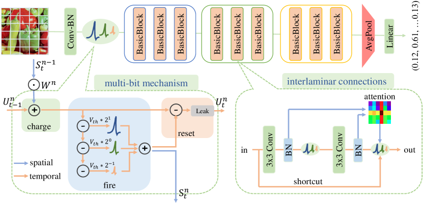
To reduce the loss during the forward process and enhance the amount of information carried by spikes, we propose a multi-bit information transmission mechanism. Futhermore, in order to preserve the information and promote the full firing of spikes across various bit positions, we introduce interlaminar connections. Specifically, as shown in Fig.2, we construct a ResNet-20 network, incorporating the multi-bit mechanism on the basis of LIF neurons, and introducing interlaminar connections in the basic block of the ResNet.
3.1 Multi-bit mechanism
We propose multi-bit mechanism. This mechanism extends the output of neurons from single-bit to multi-bit. Specifically, due to the fact that connections between two neurons (synapses) are multivalent rather than unique, we extend the spike to a fixed-point unsigned binary number with integer bits and fractional bits. Specifically, the feature space has the shape , and the original spike is a single integer bit, with the representation range being , so the overall feature space distribution is . The extended spike consists of integer bits and fractional bits, with the representation range being , thus the overall feature space distribution is . Clearly, the representation capability of the extended spikes has significantly increased.
We are not merely increasing the number of integer bits or fractional bits independently to improve spike distinguishability. Instead, we combine both aspects because they serve different purposes. In the following, we will provide a detailed explanation of the differences between them.
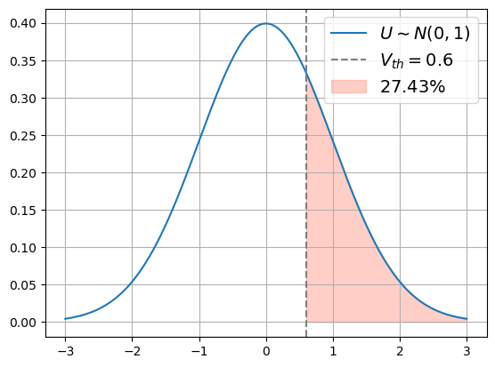
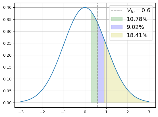
We first review the firing scenario of the basic LIF model as presented in Fig.3(a), where we assume without loss of generality that the membrane potential follows a standard normal distribution, with . We use entropy to represent the loss of information before and after firing. Before firing, the membrane potential is normally distributed. Its probability density function is
| (1) |
and its entropy is fixed, which can be described as
| (2) |
In the LIF model, the continuous is discretized into spikes, whose probabilities can be expressed as
| (3) |
where denotes the upper quantile of the normal distribution. The entropy of spikes is
| (4) |
The forward process loss of LIF is
| (5) |
The magnitude of Loss is solely determined by , as is fixed. Therefore, increasing the magnitude of is beneficial for reducing the loss in the forward process.
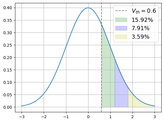
Next, let’s analyze the case of expanding the number of integer bits. Assuming an upward expansion of one bit, i.e., m=2, the range of spike values becomes {0, 1, 2, 3}. Thus, Eq.14 is transformed to
| (6) |
where represents a spike containing 2-bit integer bits, the maximum value that can be encoded is 3, thus when the membrane potential reaches three times the threshold, the maximum value of the spike is 3. The specific divisions are illustrated in Fig.3(b). The entropy can be expressed as
| (7) |
Expanding the number of integer bits does not change the quantity of spikes. Rather, it granularizes the existing spikes. This method significantly enhances the distinction of spikes, increasing the amount of information carried by them and reducing the loss in the conversion from membrane potential to spikes. However, the potential for expansion in this manner is limited, as only a very few neurons are capable of accumulating a membrane potential that exceeds several times the threshold.
Next, we analyze the expansion of spikes in terms of decimal places, as shown in Fig.3(c), which illustrates the result of expanding by one decimal place. The implementation method is similar to that of expanding the integer bits, but the effects are different. Expanding the decimal places not only allows for further granularization of the existing spikes but also enables some neurons that have not reached the threshold, yet are relatively active, to transmit part of the signal downstream. The corresponding forward process is
| (8) |
and the entropy can be expressed as
| (9) |
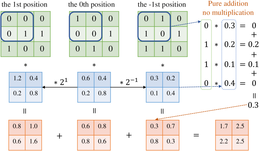
It is worth noting that the additional computational cost brought by the multi-bit mechanism is very minimal, as it does not alter the advantage of SNNs in converting MAC operations to AC operations. With the introduction of the multi-bit mechanism, the binary weights of each bit can be perfectly integrated into the parameters. SNNs still use addition for computations, as demonstrated in the Fig.4 showing the calculation process of convolutional layer parameters and multi-bit spikes.
Finally, we can calculate the entropy corresponding to the above scenarios. Clearly, as shown in Tab.1, with the bit width increases, the entropy of the spikes is increasing, which means that the information loss in converting membrane potential to spikes is decreasing.
| 0.848 | 1.149 | 1.361 | 1.998 |
3.2 Interlaminar connections
Whether it’s an ANN or an SNN, information in their network structures typically flows layer by layer. However, in real neural networks, cross-layer information fusion truly exists, known as interlaminar connections thomson2003interlaminar . Here, to further reduce the information loss in the forward process and facilitate the potential of multi-bit mechanisms, we incorporate interlaminar connections into the Basic Block of ResNet. Specifically, the original structure of the Basic Block remains unchanged, but the outputs from the two BN layers are merged before being fed into the second spiking neuron. The fusion process is illustrated in Algorithm. 1, where outputs from the two BN layers are first concatenated along the channel dimension, followed by a 1D convolution and BN. Next, the ECA module is applied to distinguish salient features while ignoring less important ones, obtaining the final fused result, which is then input into MBLIF to complete the fusion of information. It should be noted that in the fusion process, although some additional modules are introduced, apart from the 1D convolution and ECA module which have a small number of learnable parameters, the overall increase in parameters and computational cost is negligible . The entire process can be expressed as
| (10) |
| (11) |
Wherein, and respectively represent the outputs of the preceding and following BN layers, and denotes the ECA attention process as shown in Eq. 16.

Interlaminar connections not only directly enrich the network’s topological connections and enhance its expressive capabilities, but also indirectly alter the dynamical activity of spiking neurons. Specifically, on top of existing activity, newly introduced connections utilize the attention mechanism to extract effective features, which are then used to re-stimulate the neurons. As shown in Fig.5(a)-Fig.5(c), this stimulation serves as a compensation for lost information and essentially changes the original charging method of the neurons, acting as a kind of secondary charging. This means that neurons will be more fully activated; already active neurons will become even more active, and neurons that were previously inactive may also enter an active state. This encourages neurons to fully fire across all bits, fully exploiting the potential of the multi-bit information transmission mechanism.
4 Experiments
In this section, we conducted extensive experiments. Whether on static datasets or neuromorphic datasets, and whether using direct training methods or ANN-SNN conversion training, the results consistently showed improvements. Details are provided in the appendix.
4.1 Static image classification
| Work | Network | T | Accuracy |
| TSSL-BP zhang2020temporal | CIFARNet | 5 | 91.41 |
| MLF feng2022multi | ResNet-20 | 4 | 94.25 |
| tdBN zheng2021going | ResNet-19 | 2 | 92.34 |
| 4 | 92.92 | ||
| 6 | 93.16 | ||
| TET deng2022temporal | ResNet-19 | 4 | 94.44 |
| 6 | 94.50 | ||
| Ternary guo2024ternary | ResNet-20 | 2 | 94.48 |
| 4 | 94.96 | ||
| OURS | ResNet-20 | 1 | 94.59 |
| 2 | 94.75 | ||
| 4 | 94.93 | ||
| 6 | 95.00 |
| Work | Network | T | Accuracy |
| IM-LOSS guo2022loss | VGG-16 | 5 | 70.18 |
| PALIF ding2023improved | ResNet-20 | 4 | 76.09 |
| tdBN zheng2021going | ResNet-19 | 2 | 69.41 |
| 4 | 70.86 | ||
| 6 | 71.12 | ||
| TET deng2022temporal | ResNet-19 | 2 | 72.87 |
| 4 | 74.47 | ||
| 6 | 74.72 | ||
| Ternary guo2024ternary | ResNet-20 | 2 | 73.41 |
| 4 | 74.02 | ||
| OURS | ResNet-20 | 1 | 75.43 |
| 2 | 76.06 | ||
| 4 | 76.51 |
We conducted classification experiments on static data using the direct training method. Tab.2 show our experimental results on CIFAR-10krizhevsky2009learning and CIFAR-100krizhevsky2009learning , which indicate that we achieve 95.00 and 76.51 accuracy on these datasets, respectively.
4.2 Neuromorphic data classification
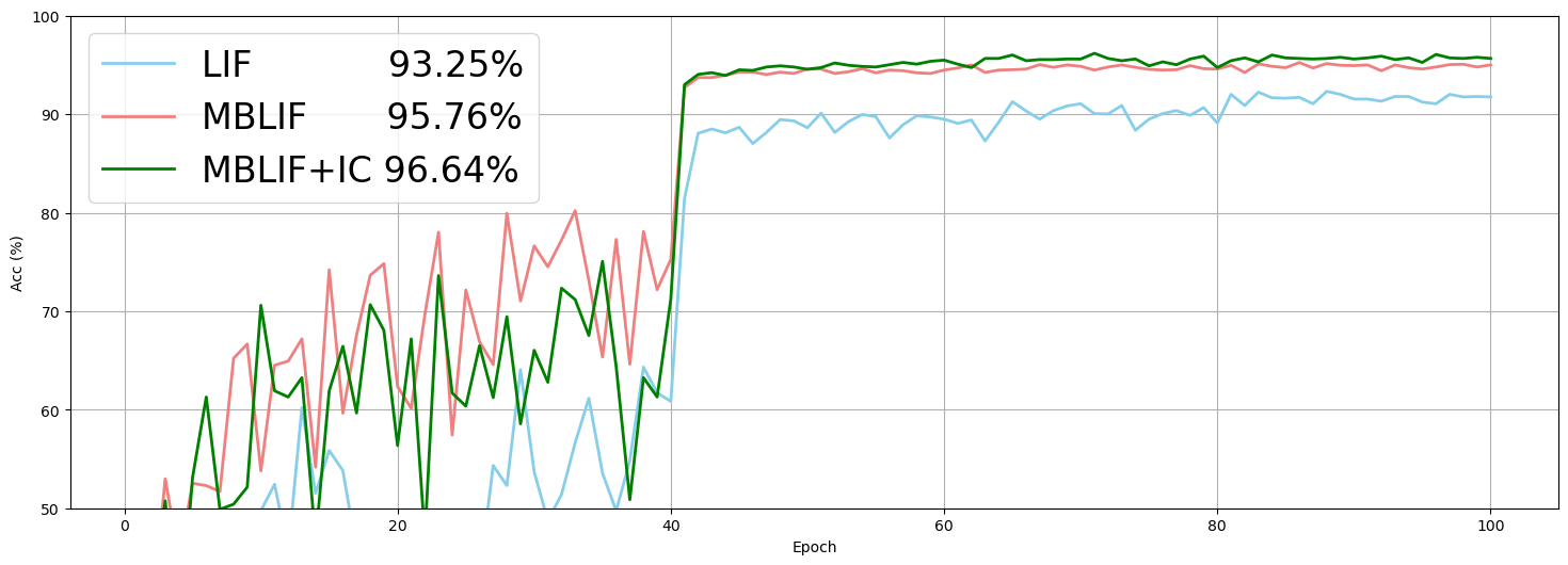
We conduct experiments on the DVS-Gesture datasetAmir2017lowpower using the direct training method. This is a more information-rich neuromorphic dataset for which we use the method of feng2022multi to preprocess data. The experimental results are shown in Fig.6. Our multi-bit mechanism results in a 2.51 increase in classification accuracy, and the interlaminar connections further increase the accuracy by 0.88. This demonstrates that our method is also applicable to neuromorphic datasets.
4.3 Ablation experiment
We conduct ablation experiments. We base our experiments on the ResNet-20 network and LIF neurons, with all parameters uniformly set: and . We particularly focus on ablating the bit width of spikes, with experimental details presented in Tab.3. It can be observed that the baseline LIF (1) results are 93.21/72.71. The expansion of bit width greatly improves the classification accuracy, with an upward expansion of one integer bit (3) leading to an increase of 1.13/2.59, a downward expansion of one fractional bit (4) resulting in a 1.23/1.77 improvement, and simultaneous expansion in both directions (5) yielding an increase of 1.40/2.94. The introduction of interlaminar connections in LIF (2) leads to an improvement of 0.48/0.62 over the baseline (1). When all settings are introduced (6), the network achieves an improvement of 1.72 on CIFAR-10 and an even more significant increase of 3.80 on CIFAR-100.
| index | Neuron | Bits | IC | CIFAR-10 | CIFAR-100 |
|---|---|---|---|---|---|
| 1 | LIF | 1 + 0 | ✗ | 93.21 | 72.71 |
| 2 | LIF | 1 + 0 | ✓ | 93.69 | 73.33 |
| 3 | MBLIF | 2 + 0 | ✗ | 94.34 | 75.30 |
| 4 | MBLIF | 1 + 1 | ✗ | 94.44 | 74.48 |
| 5 | MBLIF | 2 + 1 | ✗ | 94.61 | 75.65 |
| 6 | MBLIF | 2 + 1 | ✓ | 94.93 | 76.51 |
4.4 Performance at ultra-low time steps
Notably, as shown in Tab.4, even with just a single time step, our method remains highly competitive compared to many other works. This is primarily due to our multi-bit mechanism, which extends the bit width of spikes, trading space for time. The information contained in spikes at a single time step is significantly increased, enabling the SNN to achieve high accuracy with ultra-low time step.
| tdBN zheng2021going | TET deng2022temporal | Ternary guo2024ternary | OURS | |
|---|---|---|---|---|
| CIFAR-10 | 93.16 | 94.50 / 6 | 94.48 / 2 | 94.59 / 1 |
| CIFAR-100 | 71.12 | 74.72 / 6 | 74.02 / 4 | 75.43 / 1 |
4.5 Visualization


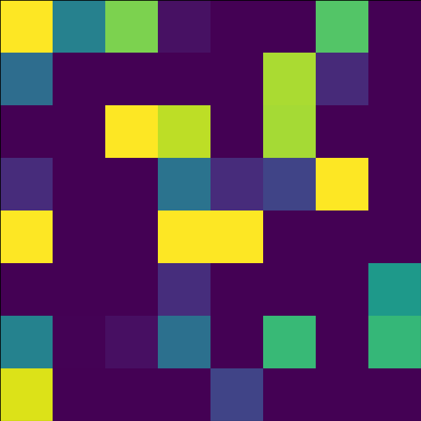
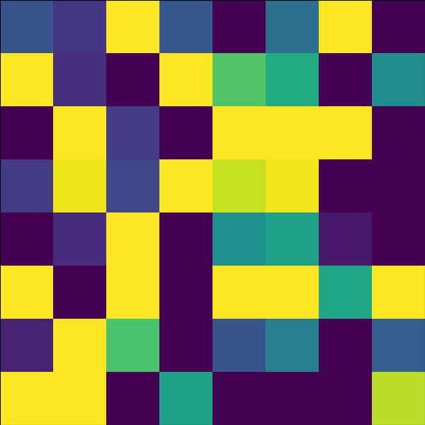
We attempt to visualize the spike firing under the multi-bit mechanism. We extract the membrane potentials of neurons in a certain layer of the network after receiving current inputs and vary the bit width of the spikes to observe the firing activity. As the bit width increases from Fig.7(a) to Fig.7(d), the entropy of the spikes significantly increases, and the details presented in the grayscale images become increasingly rich. After expanding by two bits, the entropy in Fig.7(d) rises by 132 compared to the baseline in Fig.7(a), indicating a substantial increase in the information content of the spikes.
4.6 Compared to similar ideas
As the Tab.5 shows, we compare the proposed method with some similar ideas, which mostly expand the spike, increasing its representation range. Although the basic LIF operates faster in AC operations, its information capacity is small, only representing 0,1. The extension by feng2022multi , while enhancing representational capability, reverts AC operations back to the original MAC operations, and the dynamics of neurons obviously increase the computational load, which is clearly not deployment-friendly. The ideas of zhao2022backeisnn and guo2024ternary are similar, both expanding the spike into ternary, which does not introduce much extra computation and retains the advantages of AC, but their range is limited to ternary with no further expansion space. Our multi-bit information transfer mechanism, while preserving the advantages of AC operations, also benefits from the binary nature, having nearly no increase in computation compared to the basic LIF and possesses good scalability with a wide range of feature representation capabilities.
| Work | Operation | Capacity | Explanation |
|---|---|---|---|
| BASIC | AC | original spike | |
| MLF feng2022multi | MAC | sum of of k LIF neurons | |
| BackEI zhao2022backeisnn | AC | ternary spike | |
| Ternary guo2024ternary | AC | scalable ternary spike | |
| OURS | AC | m-bit integer and n-bit fraction |
5 Conclusion
We propose a multi-bit information transmission mechanism that expands spikes from a single bit to multiple bits, greatly enriching the information content of the spikes. We also introduce interlaminar connections to facilitate the full release of spikes across various bit positions. To our knowledge, this is the first work that attempts to expand the bit-width of spikes, representing a novel information transmission paradigm for SNNs. Compared to previous models, our method introduces very few parameters yet significantly reduces the quantization loss in the forward process and still performs excellently at ultra-low time steps.
However, the increase in bit-width inevitably leads to a slight increase in spike memory usage and computation time during inference. Nevertheless, considering the reduction in information loss and the overall performance improvement, this should be tolerable. We look forward to further improvements in the future and hope that our work can inspire subsequent information transmission mechanisms, contributing to the research and development of high-precision, low-latency SNNs.
References
- [1] Alex Krizhevsky, Ilya Sutskever, and Geoffrey E Hinton. Imagenet classification with deep convolutional neural networks. Advances in neural information processing systems, 25, 2012.
- [2] David Silver, Aja Huang, Chris J Maddison, Arthur Guez, Laurent Sifre, George Van Den Driessche, Julian Schrittwieser, Ioannis Antonoglou, Veda Panneershelvam, Marc Lanctot, et al. Mastering the game of go with deep neural networks and tree search. nature, 529(7587):484–489, 2016.
- [3] Wolfgang Maass. Networks of spiking neurons: the third generation of neural network models. Neural networks, 10(9):1659–1671, 1997.
- [4] Kaushik Roy, Akhilesh Jaiswal, and Priyadarshini Panda. Towards spike-based machine intelligence with neuromorphic computing. Nature, 575(7784):607–617, 2019.
- [5] Peter U Diehl and Matthew Cook. Unsupervised learning of digit recognition using spike-timing-dependent plasticity. Frontiers in computational neuroscience, 9:99, 2015.
- [6] Alex M Thomson and A Peter Bannister. Interlaminar connections in the neocortex. Cerebral cortex, 13(1):5–14, 2003.
- [7] Qilong Wang, Banggu Wu, Pengfei Zhu, Peihua Li, Wangmeng Zuo, and Qinghua Hu. Eca-net: Efficient channel attention for deep convolutional neural networks. In Proceedings of the IEEE/CVF conference on computer vision and pattern recognition, pages 11534–11542, 2020.
- [8] Sen Song, Kenneth D Miller, and Larry F Abbott. Competitive hebbian learning through spike-timing-dependent synaptic plasticity. Nature neuroscience, 3(9):919–926, 2000.
- [9] Donald Olding Hebb. The organization of behavior: A neuropsychological theory. Psychology press, 2005.
- [10] Fangxin Liu, Wenbo Zhao, Yongbiao Chen, Zongwu Wang, Tao Yang, and Li Jiang. Sstdp: Supervised spike timing dependent plasticity for efficient spiking neural network training. Frontiers in Neuroscience, 15:756876, 2021.
- [11] Yujie Wu, Lei Deng, Guoqi Li, Jun Zhu, and Luping Shi. Spatio-temporal backpropagation for training high-performance spiking neural networks. Frontiers in neuroscience, 12:331, 2018.
- [12] Man Yao, Guangshe Zhao, Hengyu Zhang, Yifan Hu, Lei Deng, Yonghong Tian, Bo Xu, and Guoqi Li. Attention spiking neural networks. IEEE transactions on pattern analysis and machine intelligence, 2023.
- [13] Siqi Wang, Tee Hiang Cheng, and Meng-Hiot Lim. Ltmd: Learning improvement of spiking neural networks with learnable thresholding neurons and moderate dropout. Advances in Neural Information Processing Systems, 35:28350–28362, 2022.
- [14] Lin Zuo, Yi Chen, Lei Zhang, and Changle Chen. A spiking neural network with probability information transmission. Neurocomputing, 408:1–12, 2020.
- [15] Lin Zuo, Fengjie Xu, Changhua Zhang, Tangfan Xiahou, and Yu Liu. A multi-layer spiking neural network-based approach to bearing fault diagnosis. Reliability Engineering & System Safety, 225:108561, 2022.
- [16] Tong Bu, Wei Fang, Jianhao Ding, PengLin Dai, Zhaofei Yu, and Tiejun Huang. Optimal ann-snn conversion for high-accuracy and ultra-low-latency spiking neural networks. arXiv preprint arXiv:2303.04347, 2023.
- [17] Fangxin Liu, Wenbo Zhao, Yongbiao Chen, Zongwu Wang, and Li Jiang. Spikeconverter: An efficient conversion framework zipping the gap between artificial neural networks and spiking neural networks. In Proceedings of the AAAI Conference on Artificial Intelligence, volume 36, pages 1692–1701, 2022.
- [18] Seijoon Kim, Seongsik Park, Byunggook Na, and Sungroh Yoon. Spiking-yolo: spiking neural network for energy-efficient object detection. In Proceedings of the AAAI conference on artificial intelligence, volume 34, pages 11270–11277, 2020.
- [19] Hanle Zheng, Yujie Wu, Lei Deng, Yifan Hu, and Guoqi Li. Going deeper with directly-trained larger spiking neural networks. In Proceedings of the AAAI conference on artificial intelligence, volume 35, pages 11062–11070, 2021.
- [20] Yufei Guo, Yuanpei Chen, Liwen Zhang, Xiaode Liu, Yinglei Wang, Xuhui Huang, and Zhe Ma. Im-loss: information maximization loss for spiking neural networks. Advances in Neural Information Processing Systems, 35:156–166, 2022.
- [21] Lang Feng, Qianhui Liu, Huajin Tang, De Ma, and Gang Pan. Multi-level firing with spiking ds-resnet: Enabling better and deeper directly-trained spiking neural networks. In Lud De Raedt, editor, Proceedings of the Thirty-First International Joint Conference on Artificial Intelligence, IJCAI-22, pages 2471–2477. International Joint Conferences on Artificial Intelligence Organization, 7 2022. Main Track.
- [22] Dongcheng Zhao, Yi Zeng, and Yang Li. Backeisnn: A deep spiking neural network with adaptive self-feedback and balanced excitatory–inhibitory neurons. Neural Networks, 154:68–77, 2022.
- [23] Yufei Guo, Yuanpei Chen, Xiaode Liu, Weihang Peng, Yuhan Zhang, Xuhui Huang, and Zhe Ma. Ternary spike: Learning ternary spikes for spiking neural networks. In Proceedings of the AAAI Conference on Artificial Intelligence, volume 38, pages 12244–12252, 2024.
- [24] Wenrui Zhang and Peng Li. Temporal spike sequence learning via backpropagation for deep spiking neural networks. Advances in Neural Information Processing Systems, 33:12022–12033, 2020.
- [25] Shikuang Deng, Yuhang Li, Shanghang Zhang, and Shi Gu. Temporal efficient training of spiking neural network via gradient re-weighting. arXiv preprint arXiv:2202.11946, 2022.
- [26] Yongqi Ding, Lin Zuo, Kunshan Yang, Zhongshu Chen, Jian Hu, and Tangfan Xiahou. An improved probabilistic spiking neural network with enhanced discriminative ability. Knowledge-Based Systems, 280:111024, 2023.
- [27] Alex Krizhevsky, Geoffrey Hinton, et al. Learning multiple layers of features from tiny images. 2009.
- [28] Arnon Amir, Brian Taba, David Berg, Timothy Melano, Jeffrey McKinstry, John DiBenedetto, Alexander Andreopoulos, Michael Chang, Efraim DeNolf, Taposh Nayak, et al. A low power, fully event-based gesture recognition system. In Proceedings of the IEEE Conference on Computer Vision and Pattern Recognition (CVPR), pages 7243–7252. IEEE, 2017.
- [29] Alan L Hodgkin and Andrew F Huxley. A quantitative description of membrane current and its application to conduction and excitation in nerve. The Journal of physiology, 117(4):500, 1952.
- [30] L Lapicque. Recherches quantitatives sur l’excitation electrique des nerfs. J. Physiol. Paris, 9:620–635, 1907.
- [31] Eugene M Izhikevich. Simple model of spiking neurons. IEEE Transactions on neural networks, 14(6):1569–1572, 2003.
- [32] Wulfram Gerstner and Werner M Kistler. Spiking neuron models: Single neurons, populations, plasticity. Cambridge university press, 2002.
- [33] Ashish Vaswani, Noam Shazeer, Niki Parmar, Jakob Uszkoreit, Llion Jones, Aidan N Gomez, Łukasz Kaiser, and Illia Polosukhin. Attention is all you need. Advances in neural information processing systems, 30, 2017.
- [34] Dzmitry Bahdanau, Kyunghyun Cho, and Yoshua Bengio. Neural machine translation by jointly learning to align and translate. arXiv preprint arXiv:1409.0473, 2014.
Appendix A Appendix
A.1 Leaky Integrate-and-Fire model
Classic spiking neuron models include the H-H (Hodgkin-Huxley) model [29], the LIF (Leaky Integrate-and-Fire) model[30], the Izhikevich model [31], and the SRM (Spike Response Model)[32]. The LIF model has become the most widely used model among them. This model uses the charging and discharging behavior of an RC circuit to simulate a series of dynamic characteristics of neurons receiving signals and transmitting signals, and its iterative form can be expressed as follows
| (12) |
where denotes the membrane potential of the -th neuron in the -th layer at time , is time constant, is the output spike of the neuron at the previous moment, and is the input received from the previous layer. This formula can also be expanded in detail into three processes: charge, fire, and reset. The charge process is as follows
| (13) |
The equation indicates that the membrane potential accumulation at time is composed of two parts: one is the residual potential after the membrane potential leakage at at the previous time step, and the other is the external input at the current time step. Then the fire process can be described as
| (14) |
where neurons produce a spike only when the membrane potential surpasses the threshold . The final reset process can described as
| (15) |
in which the membrane potentials of neurons that have fired spikes are reset to resting potential.
A.2 Efficient Channel Attention
We used the ECA [7] mechanism to fuse signals from different layers when introducing interlaminar connections. Compared to most attention mechanisms[33, 34], this lightweight attention mechanism introduces very few parameters with one-dimensional convolution. Specifically, the ECA attention process first uses global average pooling on features to extract global information from each channel, then learns the dependencies between channels with one-dimensional convolution, and finally obtains weights with the sigmoid function. These processes can be represented as:
| (16) |
A.3 Experimental platform
The experiments were conducted on a computing platform with the following hardware specifications, as shown in Table 6.
| Component | Specification |
|---|---|
| CPU | Intel(R) Core(TM) i7-9700K CPU @ 3.60GHz |
| GPU | NVIDIA GeForce RTX 2080 Ti * 2 |
| Memory | 64 GB DDR4 RAM |
| Storage | 4 TB NVMe SSD |
| Operating System | Ubuntu 20.04.6 LTS |
| Software | Python 3.7, PyTorch 1.8.1, CUDA 11.2, cuDNN 8.1 |
A.4 Experimental setup for direct training
We apply the proposed multi-bit information transmission mechanism to LIF neurons, introduce interlaminar connections into the Basic Block of ResNet, and obtain the ResNet-20 network, which we then use for direct training and testing of the network’s performance. The hyperparameters of the each experiment are shown in the Tab.7.
| LR | Batch Size | Optimizer | Weight Decay | Epochs | Time Const | Threshold | T |
|---|---|---|---|---|---|---|---|
| 0.1 | 64 | Sgd | 100 | 4 | 0.6 | 4 |
| LR | Batch Size | Optimizer | Weight Decay | Epochs | Time Const | Threshold | T |
|---|---|---|---|---|---|---|---|
| 0.1 | 32 | Sgd | 100 | 4 | 1 | 40 |
A.5 Experiments on ANN-SNN conversion
We also test our multi-bit mechanism in ANN-SNN conversion, applying it to IF neurons. Here, instead of expanding the number of integer bits, we expand by three decimal bits, resulting in MBIF neurons that emit one integer and three decimal bits. Then, drawing on the code from [16], we build ResNet-18 and VGG-16 networks with these neurons and conduct classifications on the CIFAR-10 and CIFAR-100 datasets.
The results and comparisons with other works are shown in Tab.9. On the CIFAR-10 dataset, our method achieves nearly zero loss on the VGG-16 network with only 64 time steps, while the baseline still has some loss at 128 time steps. With our method on the ResNet-18 network, we achieve a loss of 0.1 at 128 time steps, whereas the baseline still has over 0.70 loss. On the CIFAR-100 dataset, for both VGG-16 and ResNet-18, our method significantly outperforms the baseline at 128 time steps with 64 time steps. Furthermore, our method still retains some classification ability at ultra-low time steps 4, whereas the baseline completely loses its ability to recognize images at these steps.
| Dataset | Network | Neuron | T=4 | T=16 | T=64 | T=128 | ANN |
|---|---|---|---|---|---|---|---|
| CIFAR-10 | VGG-16 | IF | - | 49.27 | 94.01 | 94.65 | 95.00 |
| MBIF(1 + 3) | - | 93.69 | 95.00 | 94.98 | |||
| ResNet-18 | IF | - | 76.31 | 94.60 | 95.25 | 95.99 | |
| MBIF(1 + 3) | 80.62 | 94.50 | 95.78 | 95.89 | |||
| CIFAR-100 | VGG-16 | IF | - | 9.12 | 59.06 | 67.66 | 74.68 |
| MBIF(1 + 3) | 15.9 | 63.14 | 73.74 | 74.32 | |||
| ResNet-18 | IF | - | 9.32 | 62.41 | 71.40 | 77.55 | |
| MBIF(1 + 3) | 37.86 | 69.88 | 76.42 | 77.06 |