The role of outflows in black-hole X-ray binaries

Abstract

Context. The hot inner flow in black-hole X-ray binaries (BHBs) is not just a static corona rotating around the black hole, but it must be partially outflowing. It is therefore a mildly relativistic “outflowing corona”. We have developed a model, in which Comptonization takes place in this outflowing corona. In all of our previous work, we assumed a rather high outflow speed of $0.8c$.

Aims. Here, we investigate whether an outflow with a significantly lower speed can also reproduce the observations. Thus, in this work we consider an outflow speed of $0.1c$ or less.

Methods. As in all of our previous work, we compute by Monte Carlo not only the emergent X-ray spectra, but also the time lags that are introduced to the higher-energy photons with respect to the lower-energy ones by multiple scatterings. We also record the angle (with respect to the symmetry axis of the outflow) and the height at which photons escape.

Results. Our results are very similar to those of our previous work, with some small quantitative differences that can be easily explained. We are again able to reproduce quantitatively five observed correlations: a) the time lag as a function of Fourier frequency, b) the time lag as a function of photon energy, c) the time lag as a function of $\Gamma$, d) the time lag as a function of the cut-off energy in the spectrum, and e) the long-standing radio – X-ray correlation. All of them with only two parameters, which vary in the same ranges for all the correlations.

Conclusions. Our model does not require a compact, narrow relativistic jet, although its presence does not affect the results. The essential ingredient of our model is the parabolic shape of the Comptonizing corona. The outflow speed plays a minor role. Furthermore, the bottom of the outflow, in the hard state, looks like a “slab” to the incoming soft photons from the disk, and this can explain the observed X-ray polarization, which is along the outflow. In the hard-intermediate state, we predict for GX 339-4 that the polarization will be perpendicular to the outflow.

1 Introduction

It is typically accepted that the broad picture of black-hole X-ray binaries (BHBs) consists of an accretion flow (a geometrically thin, cool outer disk and a geometrically thick, hot inner flow) and a narrow relativistic jet. The jet emits in the radio and the infrared, and the hot inner flow acts as a corona that up-scatters soft disk photons to produce the hard X-rays.

The energy spectrum is nicely explained in the above picture as follows: a) radio and at least part of the infrared come from the jet, b) optical, ultraviolet, and some soft X-rays come from the accretion disk, and c) hard X-rays come from the corona (for a review see Remillard & McClintock 2006). On the other hand, it is well known that the spectra of BHBs are almost infinitely degenerate, in the sense that if one is granted freedom on the geometry of the source, the selection between thermal and non-thermal electrons, their energy distribution, and the optical depth to electron scattering, almost any observed energy spectrum can be fitted.

For energies above $\sim 2$ keV, the harder photons are observed to lag with respect to softer ones. These lags have been explained as the result of propagating fluctuations in the hot inner flow (Nowak et al., 1999a; Kotov et al., 2001; Arévalo & Uttley, 2006; Uttley et al., 2011; Uttley & Malzac, 2023), light-travel times in the outflow (Reig et al., 2003), the result of impulsive bremsstrahlung injection occurring near the outer edge of the corona (Kroon & Becker, 2016), or as the evolution time-scales of magnetic flares produced when magnetic loops inflate and detach from the accretion disc (Poutanen & Fabian, 1999). However, the observed correlation of the lags with the photon-number power-law index $\Gamma$ of the hard X-rays (Kylafis & Reig, 2018; Reig et al., 2018) and with the high-energy cutoff $E_{c}$ (Altamirano & Méndez, 2015), suggest a common origin for the hard X-rays and the time lags. Likewise, the fact that the time-lag – $\Gamma$ correlation is inclination dependent (Reig & Kylafis, 2019) is also difficult to explain with the propagating-fluctuations model.

An important fact that has been neglected in the above picture is that the Bernoulli integral of the hot inner flow is positive (Blandford & Begelman, 1999). This means that the matter cannot fall into the black hole. Thus, part of the hot inner flow must escape as an outflow to leave the rest with a negative Bernoulli integral. In other words, the hot inner flow is not just a static corona rotating around the black hole, but a wind-like, “outflowing corona”.

We have been promoting the idea that the above outflow from the hot inner flow is the place where the X-ray spectrum is shaped. The reason is the following: the outflow lies above and below the hot inner flow. Thus, soft photons that are up-scattered in the hot inner flow, must, before they escape, traverse the outflow, where they continue the scattering process. Since, after a few scatterings, the photons forget their initial energy, it is the scattering in the outflow that determines the emergent X-ray spectrum.

This picture has the advantage that it is very simple. All it requires is a parabolic outflow in which Compton up-scattering of soft photons from the accretion disk takes place. No additional mechanism is required for the time lags. They come naturally with the Compton up-scattering. The harder photons are scattered more times than the softer ones, spend more time in the outflow, and therefore come out later than the softer ones. The size of the outflow and its optical depth determine the magnitude of the time lags. Also, the fact that the time lags and the hard X-ray spectrum are produced by the same process (Comptonization), means that it is not surprising that the two are correlated (Reig & Kylafis, 2015; Kylafis & Reig, 2018). Furthermore, the Comptonized X-ray spectra that come out of the outflow are anisotropic, because of the shape of the outflow (parabolic) and the outflow speed ($v_{0}=0.8c$). The harder photons come out mainly along the outflow (large optical depth) and the softer ones mainly perpendicular to it (smaller optical depth). This, then, naturally explains the inclination dependence of the time-lag – $\Gamma$ correlation (Reig & Kylafis, 2019).

The parabolic outflow also emits radio waves. In fact, the whole spectrum from radio to hard X-rays can be explained in the outflow model (Markoff et al., 2001; Giannios, 2005). In addition, since the same electrons do the Compton up-scattering and the radio emission by synchrotron, it is not surprising that the radio flux correlates with the X-ray flux (Corbel et al., 2013; Kylafis et al., 2023).

In our previous works, we used the word jet to refer to the outflow. In the past, anything outflowing was called ”jet”. This name now appears inappropriate. Our work reveals that a narrow relativistic jet is not required in this picture. There is no problem if it exists, but it is not necessary.

Here, we want to distinguish between the jet in BHXRBs, which is narrow (a few $R_{g}$ at its base, $R_{g}$ is the gravitational radius) and relativistic ($v_{0}\mathbin{\lower 3.0pt\hbox{$\hbox to0.0pt{\raise 5.0pt\hbox{$\char 62\relax$}\hss}\mathchar 29208\relax$}}0.7c$) and the outflow in BHXRBs, which is wind-like, broad ($10-10^{3}R_{g}$ at its base), and non relativistic. The outflow speed cannot be lower than the local escape speed, which is $v_{esc}(R)/c=\sqrt{2R_{g}/R}$, with $R$ the radial distance. This means that the outflow speed $v_{0}(R)$ is $>0.45c$ at $R=10R_{g}$ and $>0.045c$ at $R=10^{3}R_{g}$. Since in our previous work we used $v_{0}=0.8c$, which for a wide outflow (say $10^{2}-10^{3}R_{g}$) implies a huge mass-outflow rate, unless the matter consists of electron - positron pairs (not likely in BHBs), we need to demonstrate that an outflow with significantly lower speed reproduces the above correlations. This is what we demonstrate in the present paper, but with $v(R)=$ constant $=0.1c=v_{0}$ and not a function of $R$. The reason for this is because we do not know the mass-outflow rate at every radius $R$, in order to compute the density in the outflow at a given height as a function of radius. Thus, we feel that a demonstrative calculation, with a low constant outflow speed, will suffice. We comment about this in Sect. 2.7 and  3.

A detailed description of our model is given in Appendix A, where we also describe how our Monte Carlo code works. In Sect. 2, we discuss our results, and in Sect. 3 we give a summary and present our conclusions.

2 Results

In the next sections we present the observational results that our model is capable of reproducing. These results are to be compared with those published over the years in Reig et al. (2003), Kylafis et al. (2008), Reig & Kylafis (2015), Kylafis & Reig (2018), Reig et al. (2018), Reig & Kylafis (2019), Kylafis et al. (2020), and Reig & Kylafis (2021). Our goal is to demonstrate that a non-relativistic, wind-like outflow (i.e., $v_{0}=0.1c$) can reproduce our previous results (where a mildly relativistic outflow with $v_{0}=0.8c$ was used), which in turn, explain many observations and correlations. In this work, we have assumed that the observer sees the system at an intermediate inclination angle. Hence we combined all the escaping photons with directional cosines in the range $0.2\leq\cos\theta\leq 0.6$. A full description of the meaning of the model parameters is given in Appendix A.

Figure 1: Energy spectra for different optical depths: from top to bottom $\tau_{\parallel}=4.5,4,3.5,3,2.5,2,1.5,1$. The width at the base of the outflow was $R_{0}=400\,R_{g}$ and the Lorentz factor of the coasting electrons was $\gamma_{0}=1.14$. The spectra have been normalized by the flux at 1 keV.

2.1 Energy spectra

The observed X-ray spectral continuum (0.1–200 keV) of BHBs consists of a soft thermal component and a hard non-thermal component. The thermal component is modeled as a multi-temperature black-body and dominates the spectrum below $\sim 2$ keV (Mitsuda et al., 1984; Merloni et al., 2000). Its origin is attributed to a geometrically thin, optically thick accretion disk (Shakura & Sunyaev, 1973). The non-thermal component is well described by a power law with a high-energy exponential cutoff. This component is believed to be the result of Comptonization of low-energy photons from the accretion disk (Sunyaev & Truemper, 1979), by energetic electrons in a configuration that is still under debate.

During X-ray outbursts, BHBs go through different spectral states (McClintock & Remillard, 2006; Belloni, 2010), of which the two main ones are the soft and hard states (Done et al., 2007). Intermediate states (hard-intermediate, HIMS, and soft-intermediate, SIMS) occur when the source transits from these basic states. Each state is characterized by a different contribution of the thermal and power-law components. In the soft state (SS), the thermal black-body component dominates the energy spectrum, with no or very weak power-law emission (Remillard & McClintock, 2006; Dexter & Quataert, 2012). In this state the radio emission is quenched. In the hard state (HS), the soft component is weak or absent, whereas the power-law extends to a hundred keV or more with photon-number index $\Gamma$ in the range $1.2-2$. In the HIMS, the power-law component is still present, albeit with a steeper slope (i.e., larger $\Gamma$) than in the HS, while the black-body component starts to appear (McClintock & Remillard, 2006; Castro et al., 2014), if it was not already there in the HS. In the HS and the HIMS, the systems shine bright in the radio band.

In our model, the Comptonizing medium is the outflow, which extends laterally to relatively large distance (few hundred of $R_{g}$ at its base) from the black hole. Therefore, our model is relevant for the HS and HIMS and it should be able to reproduce a power-law with photon index in the range $1.2-2.6$, as measured in the observations.

The main parameter that affects the slope of the continuum is the optical depth $\tau_{\parallel}$ ($\tau_{\perp}$ is uinquely determined given $\tau_{\parallel}$ and $R_{0}$), as it is a parameter directly related to the number of scatterings in the outflow. Indeed, we can reproduce the observed range of photon index $\Gamma$ in the HS and the HIMS by changing the optical depth $\tau_{\parallel}$. Figure 1 shows the resulting energy spectra of our model. Each spectrum corresponds to a model with $R_{0}=400\,R_{g}$, Lorentz $\gamma_{0}=1.14$, and variable $\tau_{\parallel}$ between 1 and 4.5, while the rest of the parameters are kept fixed at the reference values given in Table 1. The spectra have been normalized by the flux at 1 keV. The non-relativistic outflow ($v_{0}=0.1c$) requires lower values of the optical depth to reproduce the photon index of the HS and HIMS, compared to the mildly relativistic outflow that we used before ($v_{0}=0.8c$), for which $\tau_{\parallel}$ ranged between 2 and 11 (Reig et al., 2003; Kylafis & Reig, 2018).

Figure 2: Time lag as a function of Fourier frequency. The model shown corresponds to $\tau_{\parallel}=3$, $R_{0}=400\,R_{g}$, and $\gamma_{0}=1.14$.

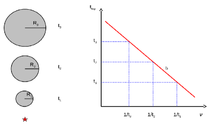
Figure 3: Explanation of the frequency dependence of time lags.

2.2 Lag-frequency correlation

When two light curves obtained at two separate energy bands (say, a hard and a soft) are cross-correlated, lags are observed between the hard and soft bands. Positive or hard lags mean that the hard photons lag the soft photons. This is always the case at energies above $\sim 2$ keV, that is, at energies where the power-law component, typically associated with Comptonization, dominates. The magnitude of this lag strongly depends on Fourier frequency and on the energy bands considered (Miyamoto et al., 1988; Vaughan & Nowak, 1997; Cui et al., 1997; Poutanen, 2001; Pottschmidt et al., 2003), but typically it is in the range of 1–100 ms. A different type of lags are the so-called reverberation or soft lags, where the soft photons (say, around 0.5 keV) lag the hard ones. These can result from the delay between the hard photons that hit the accretion disk, are absorbed there, and are emitted as soft photons, and the hard photons that reach the observer directly, before the soft photons (Uttley et al., 2014). In this case the soft band is defined at energies below $\sim 1$ keV, as it comes from the disk (Uttley et al., 2011). Reverberation lags are typically negative, that is, soft photons lag hard photons (Kara et al., 2019). This is explained by the extra path that the absorbed hard X-rays have to travel. In this work we deal with positive lags only.

The positive lags, calculated at energies above $\sim 2$ keV, can naturally be attributed to inverse Comptonization. In order to acquire their energy, harder photons scatter more times than less hard photons, hence they stay longer in the Comptonizing medium before they escape. In this context, time lags simply signify the difference in light-travel time of photons within the Comptonizing region. A different explanation of the time lags was offered by Lyubarskii (1997, see also and ). In this model, the lags result from viscous propagation of mass-accretion fluctuations within the inner regions of the accretion flow.

Observations of time-lags in the hard state show that they roughly follow a power-law dependence on Fourier frequency of the form $t_{\rm lag}\propto\nu^{-0.8\pm 0.1}$ (Crary et al., 1998; Nowak et al., 1999b; Cassatella et al., 2012). Our model reproduces quantitatively this nearly $1/\nu$ dependence of the time-lags on Fourier frequency, and this is shown in Fig. 2. The time of flight of all escaping photons was recorded in $N_{\rm bins}=8192$ time bins of duration 1/64 s each. This time was computed by adding up the path lengths traveled by each photon and dividing by the speed of light. Then, we considered the light curves of two energy bands: soft or reference band (2 - 6 keV) and hard (6 - 15 keV). We identified the phase lag $\phi$ between the signals of the two bands as the phase of the complex cross-vector, and from it the corresponding time lag $\tau=\phi/2\pi\nu$ as a function of Fourier frequency $\nu$.

The black filled circles in Fig. 2 correspond to a model with $\tau_{\parallel}=3$, $R_{0}=400\,R_{g}$, and $\gamma_{0}=1.14$. The values of these parameters are not crucial, as long as $\tau_{\parallel}$ is not too large. The case of large $\tau_{\parallel}$ will be explored in a subsequent paper (Reig, Kylafis, & Pe’er, in preparation). It is straight forward to explain qualitatively the above approximately $1/\nu$ dependence of the time-lags, because Compton scattering acts like a filter that cuts off the high frequencies. We explain this below.

For the sake of this argument, let’s think of the outflow as a series of spheres with radii $R_{1}<R_{2}<R_{3}<...$, one on top of the other, with the smaller one at the bottom (see Fig. 3). This is a discrete visualization of the parabolic outflow with radius $R(z)=R_{0}(z/z_{0})^{1/2}$, where $z_{0}$ is the height above the black hole at which the outflow starts. If $\tau_{\parallel}$ is of order unity, then soft photons from the accretion disk, that enter the outflow from below, can scatter in any of the above spheres. The source of soft input photons is indicated in Fig. 3 by a star. Consider soft photons that have an intrinsic variability with period $P$, i.e., frequency $\nu=1/P$, and scatter in one of the spheres. If they scatter in the sphere with radius $R_{1}$, this variability will be significantly reduced if the time delay due to Compton scattering, $t_{1}=R_{1}/c$, is comparable to or larger than $P$. This means that all frequencies larger than $1/t_{1}=c/R_{1}$ will be essentially washed out. If the scattering occurs in the sphere with radius $R_{2}$, with typical time delay $t_{2}=R_{2}/c$, then all frequencies larger than $1/t_{2}=c/R_{2}$ will be washed out, and so on. In other words, if the time delay due to Compton scattering is $t$, then all frequencies of variability in the input photons larger than $1/t$ will be washed out. The Monte Carlo Comptonization in a parabolic outflow reproduces the $\nu^{-\alpha}$ dependence, with $\alpha=0.7-0.9$. If the outflow is not parabolic, then Comptonization does not reproduce this frequency dependence. Such outflows will be examined in a subsequent paper and they seem to be related with the outlier sources, i.e., the sources that do not obey the regular radio – X-ray correlation (Gallo et al., 2003; Corbel et al., 2003; Kylafis et al., 2023).

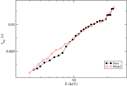
Figure 4: Lag as a function of energy. Black filled circles represent the observations for Cyg X–1. The model shown as red empty circles corresponds to $\tau_{\parallel}=2$, $R_{0}=180\,R_{g}$, and $\gamma_{0}=1.14$.

.

2.3 Lag-energy correlation

In the previous section, we showed that the hard lags observed in the HS of BHBs can be due to the fact that the harder photons have undergone more scatterings inside the outflow (the region where the energetic electrons reside) than lower-energy photons. Also, the energy of the photons changes with every scattering, with an increase in energy, on average. Therefore, both the final amplitude of the lags and the energy with which the photons escape depend on the number of scatterings. Comptonization models predict a log-linear energy dependence in the lags, approximately what is observed (Nowak et al., 1999b; Kotov et al., 2001; Stevens & Uttley, 2016). The slope of the relation depends on the range of Fourier frequencies considered to compute the average lag, becoming flatter as the frequency increases (Kotov et al., 2001; Uttley et al., 2011) Observations with good signal-to-noise show that the relation may be more complex than a simple log-linear law, with some bumps or breaks, around the energy of the iron line at 6.4 keV (Kotov et al., 2001; Stevens & Uttley, 2016).

Figure 4 shows the energy dependence of the time lag, as computed from our model with $R_{0}=180R_{g}$, $\tau_{\parallel}=2$, and $\gamma_{0}=1.14$. The data are from Kotov et al. (2001) for Cyg X–1. The reference band is 2.7–4 keV and the frequency range of the lag calculation is 0.05–5 Hz, to approximately match the values used by Kotov et al. (2001). In general terms, our model reproduces quite well the approximately linear relation between $t_{\rm lag}$ and $\log E$.

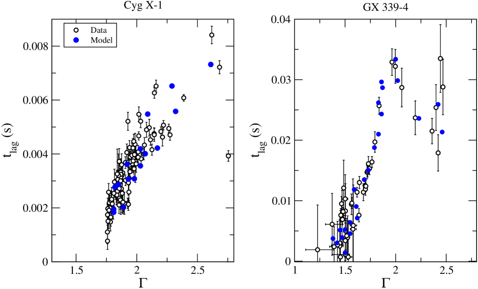
Figure 5: Correlation between time lag and photon index $\Gamma$ for Cyg X–1 (left) and GX 339–4 (right). The data for Cyg X–1 come from Pottschmidt et al. (2003, see also ) and for GX 339–4 from Kylafis & Reig (2018). Black empty circles represent the observations and the filled blue circles correspond to the models, which are produced with $\gamma_{0}=1.14$ and the values of $\tau_{\parallel}$ and $R_{0}$ that are shown in Fig. 6

.

2.4 Lag - $\Gamma$ correlation

Numerous studies have shown that the spectral (e.g., photon index $\Gamma$, cutoff energy $E_{c}$) and timing (characteristic frequency of the broad-band noise and QPOs, time or phase lags) quantities in BHBs display tight correlations (Di Matteo & Psaltis, 1999; Pottschmidt et al., 2003; Kalemci et al., 2003, 2005; Shaposhnikov & Titarchuk, 2009; Stiele et al., 2013; Shidatsu et al., 2014; Grinberg et al., 2014; Kalamkar et al., 2015; Altamirano & Méndez, 2015; Kylafis & Reig, 2018; Reig et al., 2018; Reig & Kylafis, 2019; Karpouzas et al., 2021; Méndez et al., 2022). These correlations represent convincing evidence that the timing and spectral properties of the sources are closely linked.

We have demonstrated that our outflow model is able to reproduce the observed correlation between time lag and $\Gamma$, not just for a specific source CygX–1 (Kylafis et al., 2008) or GX 339–4 (Kylafis & Reig, 2018), but in general for BHBs as a group (Reig et al., 2018). All these correlations were reproduced varying only the optical depth $\tau_{\parallel}$ and the width at the base of the outflow $R_{0}$. In those models, the Lorentz factor was $\gamma_{0}=2.24$, which resulted from a high outflow speed $v_{0}=0.8c$ and a moderate perpendicular component $v_{\perp}=0.4c$. In this work, we show that the outflow speed is not a critical parameter of the model and that a non-relativistic outflow with $v_{0}=0.1c$ can also reproduce the observations. We take $v_{\perp}=0.47c$, so that $\gamma_{0}=1.14$.

In Fig.5 we show the $t_{\rm lag}-\Gamma$ correlation for Cyg X–1 (left panel) and for GX 339–4 (right panel). The black empty circles represent the observations and the blue filled circles our models. These figures are to be compared with Fig. 2 in Kylafis et al. (2008) and Fig. 2 in Kylafis & Reig (2018). The energy and frequency ranges used to compute the lags are the same as in the above references, namely between the bands $2-4$ keV and $8-14$ keV in the frequency range $3.2-10$ Hz for Cyg X–1, and between $2-6$ keV and $9-15$ keV in the $0.05-5$ Hz range for GX 339–4. This comparison reveals that even if the outflow speed is reduced from $0.8c$ to $0.1c$, the range of variability of the optical depth $\tau_{\parallel}$ and radius $R_{0}$ does not change significantly. At the lower outflow speed ($v_{0}=0.1c$), the fits require slightly smaller optical depth and larger radius, $1\mathbin{\lower 3.0pt\hbox{$\hbox to0.0pt{\raise 5.0pt\hbox{$\char 60\relax$}\hss}\mathchar 29208\relax$}}\tau_{\parallel}\mathbin{\lower 3.0pt\hbox{$\hbox to0.0pt{\raise 5.0pt\hbox{$\char 60\relax$}\hss}\mathchar 29208\relax$}}6$ and $50\,R_{g}\mathbin{\lower 3.0pt\hbox{$\hbox to0.0pt{\raise 5.0pt\hbox{$\char 60\relax$}\hss}\mathchar 29208\relax$}}R_{0}<1500\,R_{g}$, compared to $2\mathbin{\lower 3.0pt\hbox{$\hbox to0.0pt{\raise 5.0pt\hbox{$\char 60\relax$}\hss}\mathchar 29208\relax$}}\tau_{\parallel}\mathbin{\lower 3.0pt\hbox{$\hbox to0.0pt{\raise 5.0pt\hbox{$\char 60\relax$}\hss}\mathchar 29208\relax$}}11$ and $30\,R_{g}\mathbin{\lower 3.0pt\hbox{$\hbox to0.0pt{\raise 5.0pt\hbox{$\char 60\relax$}\hss}\mathchar 29208\relax$}}R_{0}\mathbin{\lower 3.0pt\hbox{$\hbox to0.0pt{\raise 5.0pt\hbox{$\char 60\relax$}\hss}\mathchar 29208\relax$}}600\,R_{g}$ for the $v_{0}=0.8c$ case.

Figure 6: Correlation between the optical depth $\tau_{\parallel}$ and the radius $R_{0}$ of the outflow at its base for Cyg X–1 (left) and GX 339–4 (right). The values of the parameters $R_{0}$ and $\tau_{\parallel}$ are those that were used in the models that produced Fig. 5.

2.5 $\tau_{\parallel}$ - $R_{0}$ correlation

One remarkable outcome of our model is the correlation that we have found between the optical depth $\tau_{\parallel}$ and the radius $R_{0}$ at the base of the outflow (Kylafis et al., 2008; Kylafis & Reig, 2018; Reig et al., 2018; Reig & Kylafis, 2019). As we mentioned before, we can reproduce a number of observations and correlations by changing only the two basic parameters $\tau_{\parallel}$ and $R_{0}$. Surprisingly, these two parameters do not vary independently of one another, but in a correlated manner, following a power law $\tau_{\parallel}\propto R_{0}^{-\beta}$, in the HS of BHBs. Thus, for the modeling of the HS of BHBs we basically need one parameter, not two. Figure 6 shows this correlation. The points correspond to the models that were used for the explanation of the $t_{\rm lag}-\Gamma$ correlations shown in Fig. 5. The correlations break down when the source enters the HIMS. The index $\beta$ is not unique for all BHBs, but different sources display different values of $\beta$. For example, for Cyg X–1, $\beta=0.69$ and for GX  339–4, $\beta=0.38$. This is to be expected since the amplitudes of the lags of the two sources are significantly different.

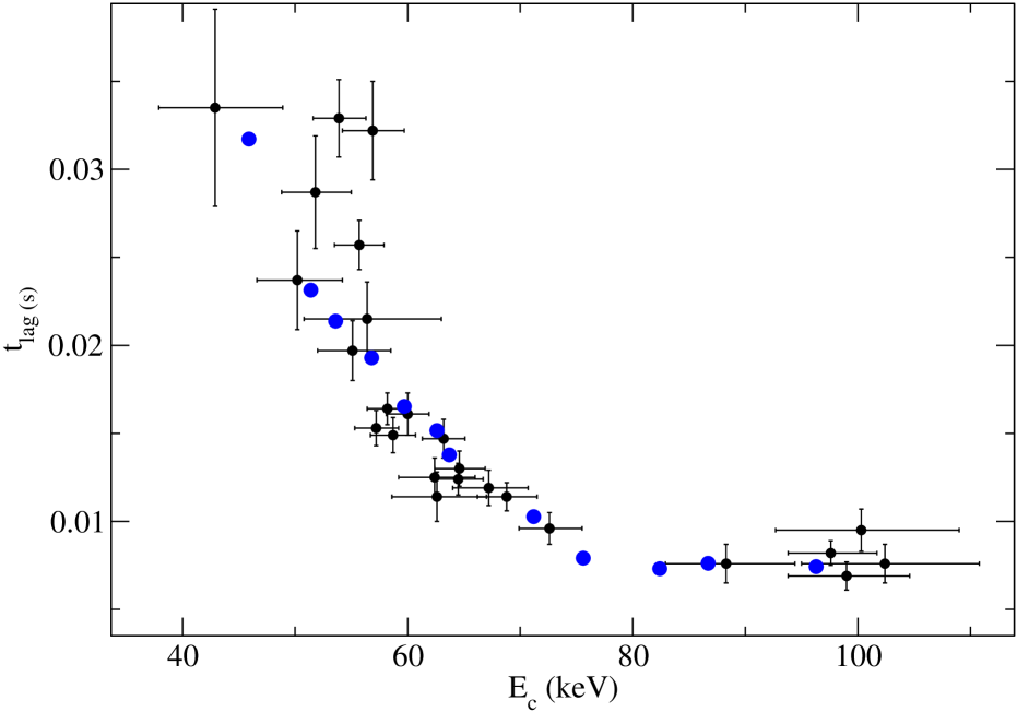
Figure 7: Relationship between the time lag and cut-off energy. Black circles represent the observations for the BHB GX 339–4. The blue circles correspond to our models. The values of the parameters $R_{0}$ and $\tau_{\parallel}$ are the same as in the models that were used in Fig. 5.

2.6 Lag – cut-off energy correlation

Another interesting result observed in the BHB GX 339–4 is the correlated evolution of the cut-off energy $E_{c}$ (in its energy spectrum) and the phase-lag $\phi_{\rm lag}$ of harder photons compared to less hard ones, as the source progresses along the HS (Motta et al., 2009; Altamirano & Méndez, 2015). As the X-ray flux increases, the cut-off energy decreases and the amplitude of the time lag increases (see Fig. 7 in Altamirano & Méndez, 2015). We showed in Sect. 2.1 that higher optical depths $\tau_{\parallel}$ result in harder spectra (the photons are scattered more and gain more energy from the energetic electrons of the outflow). Likewise, by increasing $R_{0}$, the spectrum also hardens, because larger $R_{0}$ translates to larger Thomson optical depth $\tau_{\perp}$ perpendicular to the axis of the outflow and therefore more scatterings of the photons. For the same reason, the amplitude of the lags increases when the optical depth and/or the radius of the outflow increase. The cut-off energy $E_{c}$ has a weak dependence on $\tau_{\parallel}$ and $R_{0}$, but a rather strong dependence on $v_{\perp}$. This is because the cut-off is mainly determined by the energetics of the electrons and $v_{\perp}$ determines the maximum energy gain of the soft photons (Giannios et al., 2004; Giannios, 2005).

In Reig & Kylafis (2015), we reproduced the correlation between the cut-off energy $E_{c}$ and the phase lag $\phi_{\rm lag}$ observed in the BHB GX 339–4 by changing $\tau_{\parallel}$, or $v_{\perp}$, or both in a correlated way. In that work, we kept $R_{0}$ fixed at 100 $R_{g}$. However, as the outburst progresses (i.e., as the X-ray flux increases), we expect that both $\tau_{\parallel}$ and $R_{0}$ will vary, as we have already shown in Sect. 2.4. Our model requires that as the source moves from the HS to the HIMS, $\tau_{\parallel}$ decreases and the $R_{0}$ increases.

Here we reproduce again the correlation between lag and cut-off energy in a slightly different form (Fig. 7). We use time lag instead of phase lag and the results of our own analysis instead of data from Motta et al. (2009) and Altamirano & Méndez (2015). The details of the analysis can be found in Reig et al. (2018). We use data from the 2006 outburst of GX 339–4. In Fig. 7, black filled circles represent the observations and blue filled circles the results of our models. We emphasize that the models displayed in Fig. 7 are the same models (i.e., the same combinations of $\tau_{\parallel}$ and $R_{0}$) that reproduced the $t_{\rm lag}$ – $\Gamma$ correlation of Fig. 5, simply adjusting slightly the $v_{\perp}$. The values of $v_{\perp}$ that reproduce the observations vary in the range $0.41c-0.46c$.

Figure 8: Photon index as a function of escaping direction. The blue dots are for $v_{0}=0.8c$ and the black dots for $v_{0}=0.1c$. In the inset, we show the corresponding Lorentz $\gamma_{0}$.

2.7 Inclination effects

In Reig et al. (2018), we investigated the correlation between $t_{\rm lag}$ and $\Gamma$ for a large number of BHBs. The data in the correlation showed a large scatter that was explained as an inclination effect (Reig & Kylafis, 2019). Systems seen at low inclination exhibit a stronger correlation. In high-inclination systems, the correlation is rather weak. We also showed that low- and intermediate-inclination systems tend to have harder spectra (see also Reig et al., 2003) and a larger amplitude of time lags. The explanation is that, in a mildly relativistic outflow, the high bulk speed of the electrons provides a boost on the photons that makes them scatter preferentially in the forward direction. These photons travel longer distances and suffer more scatterings than photons that escape perpendicularly to the outflow axis. Therefore, photons that escape at small to moderate angles $\theta$ with respect to the outflow axis lead to harder spectra (smaller photon index), because they undergo more scatterings and longer lags because they travel longer distances.

Figure 8 shows the dependence of the photon index on the escaping angle for the case of a mildly relativistic outflow with $v_{0}=0.8c$ (blue dots) and a non-relativistic outflow with $v_{0}=0.1c$ (black dots). Here $\theta$ is the angle between the observer and the outflow axis (i.e., photons with $\cos\theta\sim 1$ escape along the axis, while $\cos\theta\sim 0$ escape perpendicular to the outflow axis). The parameters of the models shown are $\tau_{\parallel}=5.5$ and $R_{0}=140\,R_{g}$ for the mildly relativistic outflow and $\tau_{\parallel}=3.5$ and $R_{0}=150\,R_{g}$ for the non-relativistic outflow.

As we indicated in the Introduction, our model with constant $v_{0}=0.1c$ is only demonstrative because in reality the escape speed is not expected to be constant, but a function of $R$, and it ranges from $0.58c$ at $R=6R_{g}$ to $0.045c$ at $R=10^{3}R_{g}$. Thus, the real outflow has a central fast part and a progressively slower outer part. Without this variable $v_{0}(R)$ it is not possible to compute accurately the spectra as a function of inclination.

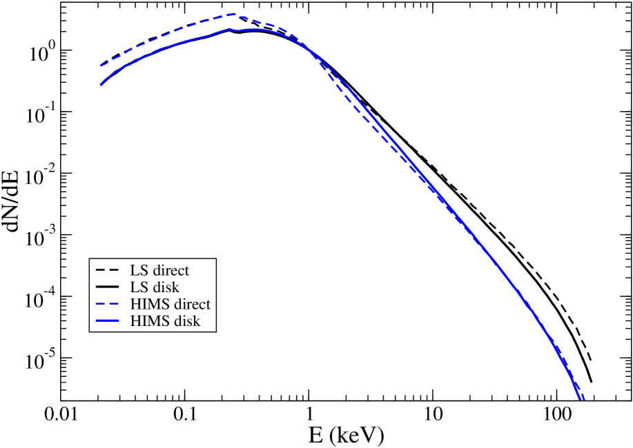
Figure 9: Comparison of the “direct” and “disk” spectra. The direct spectrum is the spectrum seen by observers at infinity at an inclination $\theta\sim 40^{\circ}$ and the “disk” spectrum is the spectrum of the photons that are back-scattered and illuminate the disk. The parameters of the models used in this figure for the LS are $\tau_{\parallel}=2.5$, $R_{0}=500$ $R_{g}$, and $\gamma_{0}=1.14$ and for the HIMS $\tau_{\parallel}=1.5$, $R_{0}=1400$ $R_{g}$, and $\gamma_{0}=1.14$.

2.8 Disk illumination

In our model, soft photons are injected isotropically upward at the base of the outflow. Depending on $\tau_{\parallel}$ and the initial direction, photons may escape unscattered or after a number of scatterings. After escape, we record their energy, angle of escape (with respect to the outflow axis), height from the black hole, and travel time in the outflow. Hence, the code also computes the back-scattered photons, i.e., photons with escaping angle $\theta>\pi/2$. Some of these photons will be absorbed by the accretion disk and others will be reflected by it. The code, in its current version, does not account for reflection, but we can measure the number of photons that hit the accretion disk. In other words, we can compute the irradiation spectrum.

In Reig & Kylafis (2021), we showed that the fraction of back-scattered photons increases as the Lorentz factor $\gamma_{0}$ decreases. The reason is that in non relativistic outflows the scattering is nearly isotropic, whereas when the outflow velocity is high, there is a strong forward boost, as explained in the previous section. Although in our model photons can interact with electrons anywhere in the outflow, most of the scatterings occur close to the black hole, not far away from the base of the outflow if the outflow velocity is low.

Fig. 9 compares the energy distribution of the photons that illuminate the disk, that is the “disk” spectrum (solid line), with the “direct” spectrum of the photons from the outflow, seen by observers for typical LS and HIMS spectra. Unlike the relativistic case with $v_{0}=0.8c$, where the “disk” spectrum was much softer than the “direct” one (see Fig. 3 of Reig & Kylafis, 2021), here the “disk” and the “direct” spectra are very similar. The spectra, both “direct” and “disk”, are slightly softer in the HIMS than in the HS, in agreement with observations.

Another way to investigate the irradiation of the accretion disk by the primary source is by computing the emissivity profile, which is the radially dependent flux irradiating the disk by the source. For a standard Shakura-Sunyaev accretion disk, it is parameterized as a power law $F(r)\propto r^{-q}$, with $q$ the emissivity index. The standard behavior is $q=3$ (Dauser et al., 2013). To compute the emissivity index, we divided the accretion disk into radial zones and computed the number of photons per unit area that irradiate a given zone. For the sake of the computation and in order to compare with the lamppost geometry, we collapsed the outflow to $R_{0}=1\,R_{g}$. We find that for $R_{\rm disk}\mathbin{\lower 3.0pt\hbox{$\hbox to0.0pt{\raise 5.0pt\hbox{$\char 62\relax$}\hss}\mathchar 29208\relax$}}10\,R_{g}$, the radial dependence of the irradiated flux on the disk does follow a power-law with $q=3$, that is, the expected value for a standard Shakura-Sunyaev disk.

Fig. 10 shows the distribution of distances $h$ from the black hole from which the photons that hit the accretion disk escape. We show this distribution for different values of $\tau_{\parallel}$ (top panel) and $R_{0}$ (bottom panel) and two Lorentz factors $\gamma_{0}=1.10$ and $\gamma_{0}=2.24$ (i.e., $v_{0}=0.1c$ and $v_{0}=0.8c$, respectively). As expected, most of the photons escape within a few $R_{g}$, but a significant fraction of the photons that hit the accretion disk also escape at tens to few hundreds of $R_{g}$. This figure also confirms the fact that disk illumination increases as the outflow speed decreases. The vertical axis in Fig. 10 is reminiscent of the reflection fraction, defined as the number of emitted photons of the primary source which hit the accretion disk $N_{\rm AD}$ over the number of photons escaping to infinity $N_{\infty}$ (Dauser et al., 2014, 2016). .

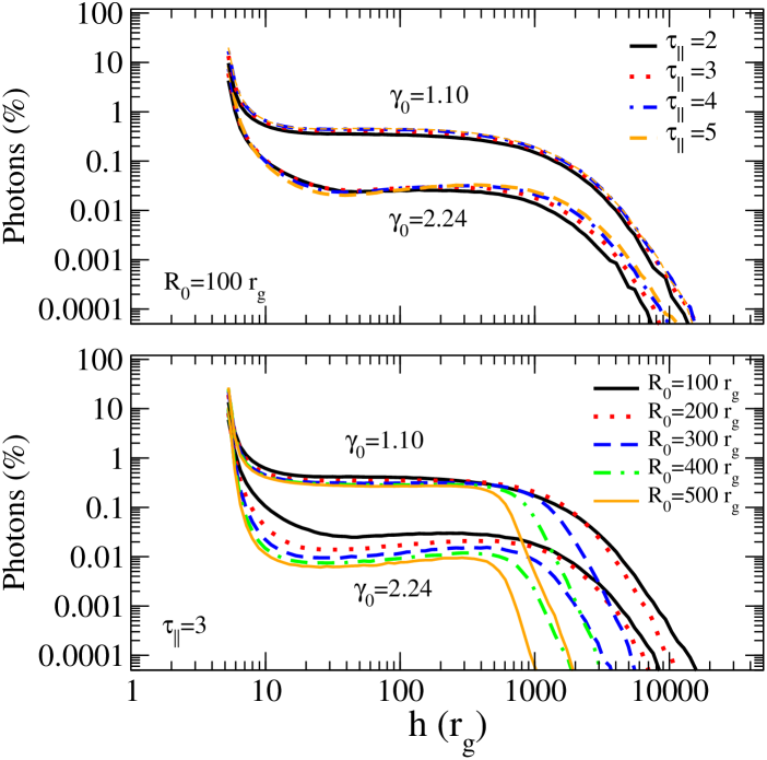
Figure 10: Fraction of photons that hit the accretion disk over the total number of photons as a function of distance $h$ from the black hole at which they escape, for different values of the optical depth $\tau_{\parallel}$ and radius $R_{0}$ of the outflow. The distribution is shown for a mildly relativistic outflow ($\gamma_{0}=2.24$, i.e., $v_{0}=0.8c$) and non relativistic outflow ($\gamma_{0}=1.10$, i.e., $v_{0}=0.1c$).

Figure 11: Radio–X-ray flux correlation for GX 339–4. The models used to compute the radio flux and the theoretical $\Gamma$ are the same as those that reproduce the time lag–$\Gamma$ correlation displayed in Fig. 5.

2.9 The radio – X-ray correlation

One of the most tight correlations in BHBs is the radio–X-ray correlation (Hannikainen et al., 1998; Corbel et al., 2000, 2003; Gallo et al., 2003; Bright et al., 2020; Shaw et al., 2021). The correlation extends over five orders of magnitude in radio flux and eight orders of magnitude in X-rays. The radio – X-ray correlation is in the form of a power-law $F_{R}\propto F_{X}^{\delta}$, where $\delta\approx 0.5-0.7$ (Gallo et al., 2012; Corbel et al., 2013). In addition to the main correlation, a group of outliers populate the $F_{R}-F_{X}$ plane (Gallo et al., 2012). The group of outliers is associated with radio quiet sources, while most of the sources that follow the standard correlation are radio loud systems (Espinasse & Fender, 2018). This difference in radio emission could be an inclination effect (Motta et al., 2018), though other possibilities should be examined. Here we show that our model can reproduce the standard $F_{R}-F_{X}$ correlation. In particular, for the best-studied BHB GX 339–4, for which the correlation stands for more than five orders of magnitude in X-ray flux, the exponent is $\delta=0.62\pm 0.01$ (Corbel et al., 2013).

We follow the same procedure as in Kylafis et al. (2023), where we reproduced the $F_{R}-F_{x}$ correlation for the case of a mildly relativistic outflow, i.e., $v_{0}=0.8c$. From the X-ray observations of the 2007-2008 outburst of GX 339-4, we obtained a relationship between X-ray flux and photon-number spectral index $\Gamma$. We rebinned the data in bins of 0.05 in $\Gamma$ for the HS and 0.1 for the HIMS. The error in the flux was computed as the standard deviation of the data in each bin. From our model, we computed the radio flux and the X-ray spectrum, i.e., the spectral index $\Gamma$, for each set of input parameters $(R_{0},\tau_{\parallel})$. Thus, we obtained an entirely theoretical relationship between radio flux and photon index $\Gamma$. We stress that our model input parameters are not arbitrary, but they are exactly the same as those in Fig. 6 (right panel), which reproduce the correlation between time lag and $\Gamma$, shown in Fig. 5 (right panel). Thus, we attempt to explain two correlations with the same model parameters.

From the observed $F_{X}-\Gamma$ correlation and the computed $F_{R}-\Gamma$ one, we matched the radio and X-ray fluxes that have the same or very similar value of $\Gamma$, and plotted one against the other. The result is shown in Fig. 11. We refer the reader to Appendix A (see also Giannios, 2005; Kylafis et al., 2023) for the computation of the radio flux with our model as well as the details of the analysis of the X-ray observations. The black line Fig. 11 is not a fit to the blue dots, but it is the observational correlation of (Corbel et al., 2013). The blue dots correspond to the HS and the red dots to the HIMS. The only quantity that we had to change in this calculation, as compared with the one reported in Kylafis et al. (2023), is the magnetic field $B_{0}$ at the base of the outflow. Here, its value is $2.9\times 10^{4}$ G.

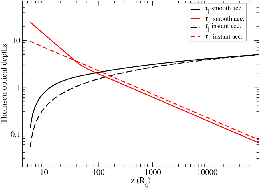
Figure 12: Thomson optical depths (parallel and perpendicular to the outflow) as functions of distance from the black hole. We show two cases: instant acceleration of the outflow (dashed lines) and when an acceleration region is present, i.e., smooth acceleration (solid lines). We used a model with $\tau_{\parallel}=5$ and $R_{0}=100$ $R_{g}$, where $R_{g}$ is the gravitational radius.

2.10 X-ray polarization

Recent results from the Imager X-ray Polarimetry Explorer (IXPE) mission (Weisskopf et al., 2022) have revealed that BHBs show polarization degrees in the X-ray band (2-8 keV) of a few percent and the polarization angle is aligned with the outflow (Krawczynski et al., 2022; Veledina et al., 2023; Ingram et al., 2023; Rodriguez Cavero et al., 2023). Since Comptonization in a slab (with Thomson optical depth in the plane of the slab much larger than in the perpendicular direction) gives rise to linear polarization perpendicular to the slab (Poutanen et al., 1996; Schnittman & Krolik, 2010), people typically assume the Comptonizing corona to be in the form of a slab, perpendicular to the outflow, but without giving a physical justification for this. Also, models with a static Comptonizing region predict a lower polarization degree than the observed one. One way to produce higher polarization is by assuming that the inner disk is viewed at a higher inclination angle than the outer disk (Krawczynski et al., 2022). Another way is by considering an outflowing Comptonizing medium (Poutanen et al., 2023; Ratheesh et al., 2023).

Our model of a parabolic, outflowing corona naturally provides a Comptonizing, outflowing “slab” at its bottom. This is shown below, where, for simplicity of the expressions, we consider an instantaneous acceleration of the outflow to speed $v_{0}$ at the bottom of it. For the full model with an acceleration region, the optical depths are calculated in Appendix A.

For a parabolic outflow, the radius of the outflow at height $z$ is

$$R(z)=R_{0}(z/z_{0})^{1/2},$$

where $R_{0}$ is the radius at the base of the outflow, which is at height $z_{0}$. From the continuity equation

$$2\pi R(z)^{2}n_{e}(z)m_{p}v_{0}=\dot{M},$$

where $n_{e}$ is the electron number density, $m_{p}$ is the proton mass, and $\dot{M}$ is the mass-outflow rate, one gets for the electron density

$$n_{e}(z)=n_{0}(z_{0}/z),$$

where $n_{0}$ is the density at $z_{0}$. The Thomson optical depth $\tau_{\parallel}(z)$ from $z_{0}$ to $z>z_{0}$ is

$$\tau_{\parallel}(z)=\int_{z_{0}}^{z}n_{e}(z)\sigma_{T}dz=n_{0}\sigma_{T}z_{0}\ln(z/z_{0}),$$

while the perpendicular Thomson optical depth at height $z$ is

$$\tau_{\perp}(z)=n_{e}(z)\sigma_{T}R(z)=n_{0}(z_{0}/z)\sigma_{T}R_{0}(z/z_{0})^{1/2}$$

$$\phantom{\tau_{\perp}(z)=n_{e}(z)\sigma_{T}}=n_{0}\sigma_{T}R_{0}(z_{0}/z)^{1/2},$$

or

$$\tau_{\perp}(z)={R_{0}\over z_{0}}{{(z_{0}/z)^{1/2}}\over{\ln(z/z_{0})}}\tau_{\parallel}(z).$$

The ratio of the optical depth $\tau_{\parallel}(z)$ to the total optical depth along the outflow $\tau_{\parallel}(H)\equiv\tau_{\parallel}$ is

$${{\tau_{\parallel}(z)}\over{\tau_{\parallel}}}={{\ln(z/z_{0})}\over{\ln(H/z_{0})}},$$

which means that

$$\tau_{\parallel}(z)={{\ln(z/z_{0})}\over{\ln(H/z_{0})}}\tau_{\parallel}.$$

Here $H$ is the height of the outflow that we take it to be $H=10^{5}R_{g}$, where $R_{g}$ is the gravitational radius.

Figure 12 shows the variation of the parallel $\tau_{\parallel}$ and the perpendicular $\tau_{\perp}$ optical depths as functions of distance $z$ from the black hole, when an acceleration region is present (i.e., the physical case, solid lines, Appendix A) and when it is absent (i.e. the non-physical, but simpler, case of instant acceleration, dashed lines). Figure 12 implies that, at its bottom, the outflow behaves like a slab, because $\tau_{\perp}>>\tau_{\parallel}$. In Sect. 2.8 (see also Fig. 10) we indicated that most of the scatterings occur near the bottom of the accretion flow, especially in the HS, because the optical depth is high. Thus, in the HS, the bottom of the outflow is seen by the incoming soft photons as an “outflowing slab” and therefore the X-ray polarization is expected to be along the outflow. In the HIMS, on the other hand, the outflowing corona (at least for GX 339-4) is nearly transparent ($\tau_{\parallel}\sim 1$). The soft photons travel along the outflow and scatter on average once. Thus, in the HIMS, the X-ray polarization is expected to be perpendicular to the outflow.

3 Summary and conclusion

We have demonstrated that we can reproduce most of the results from our previous works even with a non-relativistic outflow. These are: i) the energy spectrum (Fig. 1), ii) the dependence of the time-lag on Fourier frequency (Fig. 2), iii) the log-linear dependence of the time lag on photon energy, iv) the correlation between the time lag and the photon index $\Gamma$ in GX 339–4 and Cyg X–1 (Fig. 5), v) the time-lag – cutoff-energy correlation observed in GX 339–4 (Fig. 7), and vi) the fact that the outflow provides a natural lamp post for the hard X-ray photons that return to the disk (Fig. 10).

The reduction of the outflow speed implies that the fraction of back-scattered photons increases and their spectrum displays about the same $\Gamma$ as the photons directly escaping to the observer (unlike the models with $v_{0}=0.8c$, which produce softer spectra for the photons that return to the disk compared to those that go directly to the observer). This is because the boost in the forward direction is highly reduced. Hence the number of photons that travel at larger distances decreases. Owing to the smaller boost along the outflow axis in the case of $v_{0}=0.1c$, as compared to the case of $v_{0}=0.8c$, there is little inclination dependence of the photon index (Fig. 8), as expected. A more realistic calculation would require a parabolic outflow with a distribution of outflow velocities that decreases as one moves away from the axis. In other words, the outflow should be composed of a mildly relativistic and narrow part at its core and a less and less relativistic outflow at larger transverse distances.

As in the case of a mildly relativistic outflow ($v_{0}=0.8c$), our model with $v_{0}=0.1c$ reproduces the observations by changing only two parameters: the optical depth along the outflow axis $\tau_{\parallel}$ and the radius $R_{0}$ at its base, and these two parameters are correlated (Fig. 6), so our model has only one parameter. Our simulations in the present work ($v_{0}=0.1c$ and for GX 339–4) require a slightly smaller range in optical depth ($1\mathbin{\lower 3.0pt\hbox{$\hbox to0.0pt{\raise 5.0pt\hbox{$\char 60\relax$}\hss}\mathchar 29208\relax$}}\tau_{\parallel}\mathbin{\lower 3.0pt\hbox{$\hbox to0.0pt{\raise 5.0pt\hbox{$\char 60\relax$}\hss}\mathchar 29208\relax$}}6$) and a slightly larger range in outflow radius ($50\mathbin{\lower 3.0pt\hbox{$\hbox to0.0pt{\raise 5.0pt\hbox{$\char 60\relax$}\hss}\mathchar 29208\relax$}}R_{0}/R_{g}\mathbin{\lower 3.0pt\hbox{$\hbox to0.0pt{\raise 5.0pt\hbox{$\char 60\relax$}\hss}\mathchar 29208\relax$}}1.5\times 10^{3}$) compared to the $v_{0}=0.8c$ case for which $2\mathbin{\lower 3.0pt\hbox{$\hbox to0.0pt{\raise 5.0pt\hbox{$\char 60\relax$}\hss}\mathchar 29208\relax$}}\tau_{\parallel}\mathbin{\lower 3.0pt\hbox{$\hbox to0.0pt{\raise 5.0pt\hbox{$\char 60\relax$}\hss}\mathchar 29208\relax$}}11$ and $30\mathbin{\lower 3.0pt\hbox{$\hbox to0.0pt{\raise 5.0pt\hbox{$\char 60\relax$}\hss}\mathchar 29208\relax$}}R_{0}/R_{g}\mathbin{\lower 3.0pt\hbox{$\hbox to0.0pt{\raise 5.0pt\hbox{$\char 60\relax$}\hss}\mathchar 29208\relax$}}600$. The mass-outflow rate is of the order of $1-5$ times the Eddington rate for a 10 solar-mass black hole in the HS and $10-50$ times the Eddington rate in the HIMS. We remark, however, that the simplifying assumption of constant outflow speed makes the numbers unreliable. Future calculations, with a realistic outflow speed as a function of radius, will address this issue properly.

Finally we note that in the HS (no matter what the outflow speed is), the bottom of the outflow, where most of the scatterings occur, is like a “slab”, which produces X-ray polarization parallel to the outflow. In the HIMS and for GX 339–4, for which $\tau_{\parallel}$ is of order unity, we predict that the polarization will be perpendicular to the outflow.

Appendix A Description of the model

A.1 Introduction

Our model simulates with Monte Carlo the process of Comptonization in an outflow of matter, ejected in BHBs from the hot inner flow in the vicinity of the black hole, perpendicular to the accretion disk. Because the Bernoulli integral of the hot inner flow is positive (Blandford & Begelman 1999), the matter cannot fall into the black hole, hence part of the hot inner flow must escape as an outflow. In other words, the hot inner flow is not just a static corona rotating around the black hole, but a wind-like, “outflowing corona”. The thin accretion disk in the accretion flow is the source of blackbody photons at the base of the outflow. These soft photons either escape uscattered or are scattered in the outflow and have their energy increased, on average. This upscattering of the soft blackbody photons produces the hard X-ray power law. Furthermore, the same upscattering causes an average time lag of the harder photons with respect to the softer ones.

A.2 Morphology

Observational studies of the collimation of jets in active galactic nuclei (AGN) have shown that a large fraction of near-by AGN start with a parabolic outflow, which changes to a conical one further out (Asada & Nakamura 2012; Kovalev et al. 2020). Invoking the morphological similarity between AGN and BHBs, we assume that the outflow in BHBs has a parabolic form or something close to it. Therefore, we model the radius of the outflow, as a function of height $z$ from the black hole, as

$$R(z)=R_{0}\leavevmode\nobreak\ (z/z_{0})^{\beta},$$ (1)

where $R_{0}$ is the radius of the outflow at its base, which is taken to be at a distance $z_{0}$ from the black hole. We take the index $\beta$ to be $1/2$, though values close to it do not produce different results.

A.3 Outflow acceleration

At the bottom of the outflow, there must be an acceleration region ($z_{0}\leq z\leq z_{1}$), beyond which the flow speed is constant and equal to $v_{0}$. Thus, the speed of the outflowing matter along the $z$ axis is taken to be

$$v_{\parallel}(z)=\cases{v}_{0}\leavevmode\nobreak\ (z/z_{1})^{a},&z_{0}\leq z\leq z_{1}\\ v_{0},z>z_{1},{}$$ (2)

where we take $a=1/2$, though its exact values is not crucial.

A.4 Optical depths

If $n_{e}(z)$ is the number density of electrons along the outflow, mass conservation requires that

$$\dot{M}=2\pi R^{2}(z)m_{p}n_{e}(z)v_{\parallel}(z),$$ (3)

where the factor 2 is for both sides of the outflow, $\dot{M}$ is the total mass-outflow rate, and $m_{p}$ is the proton mass. The outflowing matter is considered to be consisting of protons and electrons only. Eqs. (1, 2, and 3) imply that the number density of electrons along the outflow is given by

$$n(z)=\cases{n}_{1}\leavevmode\nobreak\ (z_{1}/z)^{a+1},&z_{0}\leq z\leq z_{1}\\ n_{1}\leavevmode\nobreak\ (z_{1}/z),z>z_{1},{}$$ (4)

where $n_{1}$ is the number density of electrons at $z_{1}$, while the density at the base of the outflow is $n_{0}=n_{1}(z_{1}/z_{0})^{a+1}$.

The Thomson optical depth of the outflow along $z$ is given by

$$\tau_{\parallel}=\int_{z_{0}}^{H}n_{e}(z)\sigma_{T}dz$$ (5)

where $\sigma_{T}$ is the Thomson cross section and $H$ is the height of the outflow. Using Eq. (4) we find

$$\tau_{\parallel}={{n_{1}\sigma_{T}z_{1}}\over a}\left[(z_{1}/z_{0})^{a}-1\right]+n_{1}\sigma_{T}z_{1}ln(H/z_{1}).$$ (6)

Instead of $n_{0}$, we take $\tau_{\parallel}$ as a model parameter. Thus, our two main parameters are $\tau_{\parallel}$ and $R_{0}$.

The Thomson optical depth $\tau_{\parallel}(z)$ from $z_{0}$ to $z$, $z_{0}<z<H$ is

$$\tau_{\parallel}(z)=\int_{z_{0}}^{z}n_{e}(z)\sigma_{T}dz$$ (7)

or

(21)