Synthetic Data for Robust Identification of Typical and Atypical Serotonergic Neurons using Convolutional Neural Networks

Abstract

Serotonergic neurons in the raphe nuclei exhibit diverse electrophysiological properties and functional roles, yet conventional identification methods rely on restrictive criteria that likely overlook atypical serotonergic cells. The use of convolutional neural network (CNN) for comprehensive classification of both typical and atypical serotonergic neurons is an interesting one, but the key challenge is often given by the limited experimental data available for training. This study presents a procedure for synthetic data generation that combines smoothed spike waveforms with heterogeneous noise masks from real recordings. This approach expanded the training set while mitigating overfitting of background noise signatures. CNN models trained on the augmented dataset achieved high accuracy (96.2% true positive rate, 88.8% true negative rate) on non-homogeneous test data collected under different experimental conditions than the training, validation and testing data.

1 Introduction

Serotonergic neurons of the raphe nuclei play an important role in regulating diverse brain functions and behaviors, including mood, cognition, sleep, appetite, and pain modulation (Okaty et al., 2019). However, the serotonergic system is highly heterogeneous, comprised of subpopulations of neurons with distinct anatomical projections, neurochemistry, physiology, and functional roles. Elucidating the diversity of serotonergic neurons is essential to understand how modulatory control of brain states emerges from serotonergic network dynamics. Traditionally, serotonergic neurons have been identified in electrophysiology studies based on “typical” extracellular spiking characteristics, namely, slow regular firing and long spike duration (Vandermaelen and Aghajanian, 1983). While useful, these criteria likely overlook atypical serotonergic neurons, introducing a selection bias that limits insights into the full diversity of the serotonergic system (Otaky et al., 2019; Calizo et al., 2011). Deep learning methods like convolutional neural networks (CNNs) offer a powerful alternative for serotonergic neuron identification. By learning distinctive spike waveform features, CNNs can accurately discriminate both typical and atypical serotonergic neurons from non-serotonergic cells (Corradetti et al., 2024). However, developing robust CNN models for recognizing serotonergic cells from recordings poses practical challenges since large datasets from identified neurons are required for model training, while experimental recordings from serotonergic neurons, identified by methods independent of the signal recordings, are typically limited to hundreds of cells. A first way of overcoming the problem would be through the use of a naive data augmentation, extracting short segments as surrogate samples from each recording, thus increasing by one or two orders of magnitudes the number of labeled samples. Unfortunately, directly augmenting a limited number of recordings risks is a huge source of overfitting. A key role in this phenomenon is represented by the specific noise signature of the experiment which characterize all the experiments and that is therefore learned by the model in order rather than meaningful action potential features. This study addresses the challenges in developing a deep learning model for atypical serotonergic cell recognition using synthetic data generation. Indeed, this work shows that carefully designed synthetic data augmentation from limited electrophysiology data can be of use in the development of deep learning models with high accuracy recognition (Corradetti et al. 2024). The paper is structured as follows. Section 2 discusses the limitations of traditional visual identification methods for serotonergic neurons, while Section 3 examines the problems in applying straightforward deep learning approaches mainly due to the issue of limited experimental data. Section 4 presents a methodology for generating synthetic data to augment the training set. Section 5 describes a practical case study implementing the approach. Finally, Section 6 concludes the paper and discusses future research directions.

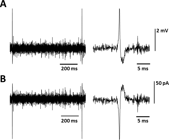
Figure 1: Appearance of extracellularly recorded action potentials according to the recording arrangement. A. Spikes from a serotonergic neuron recorded in voltage recording configuration, typically used in vivo or in vitro with sharp microelectrodes. Left trace shows two spikes on a slow recording timebase. Note the predominance of background noise over the spikes in the recorded segment. Right trace shows one of the spikes at faster timebase. Note the rapid positive upstroke followed by a negative phase comprising two subsequent downstrokes. B. Appearance of the same signals as obtained with the loose-seal patch-clamp current recording configuration used in the present work.

2 Limitations of Visual Identification Methods

Serotonergic neurons have historically been identified in electrophysiology studies using subjective visual criteria centered on “typical” spiking characteristics. The most commonly applied criteria include spike shape, spike duration, and regularity of firing (Vandermaelen and Aghajanian 1983). Idealized serotonergic neurons exhibit polyphasic spikes with an initial fast deflection followed by one or two slower deflections in the opposite direction (see e.g. Fig. 1). Spike duration, measured from initial rise to second downstroke, is relatively long, generally >1.2,ms. Firing is regular at slow rates around 0.5-2.5 Hz. Neurons meeting all these criteria can be classified as serotonergic with high confidence. However, sole reliance on these restrictive “typical characteristics” overlooks the diversity of firing patterns and spike morphologies across serotonergic subpopulations. Recordings in brain slices from genetically-identified serotonergic neurons revealed a distribution of spike durations spanning 0.5 ms to >3 ms, with many neurons exhibiting spikes narrower than the 1.2 ms criterion (Mlinar et al., 2016; Corradetti et al., 2024). While the overall distribution skews towards longer durations, nearly a third of genetically-confirmed serotonergic neurons have spike widths resembling conventional non-serotonergic neurons. Firing regularity also varies significantly. Most serotonergic neurons display regular, slow firing. But burst firing, rhythmic oscillations, and irregular patterns are observed in certain subpopulations (Hajós et al., 1995; Calizo et al., 2011; Mlinar et al., 2016). Diversity in firing likely reflects differences in inputs and intrinsic membrane properties between anatomical groups. Again, many serotonergic neurons exhibit firing indistinguishable from conventional non-serotonergic cells. Reliance on narrow spike criteria also overlooks spike shape variations in serotonergic neurons. While triphasic spikes are quite typical, spikes range from biphasic to polyphasic (Mlinar et al., 2016). Non-serotonergic neurons likewise display considerable variability in spike shape, including broad spikes resembling serotonergic morphologies.

These data demonstrate the insufficiency of restrictive visual criteria for comprehensively identifying serotonergic neurons in electrophysiology recordings. Sole reliance on “typical characteristics” such as measuring the upstroke/downstroke interval (UDI) may result not indicative enough for immediate serotonergic neuron identification and introduces a strong selection bias that likely overlooks much of the diversity of serotonergic neuron physiology and function. Researchers adhering strictly to conventional spike criteria may discard neurons that are genuinely serotonergic but exhibit narrower spike width, irregular firing, or atypical shape. This precludes studying how functional differences between serotonergic subpopulations emerge from heterogeneity in spiking characteristics and intrinsic properties. Conversely, non-serotonergic neurons with spike width and shape similar to conventional serotonergic criteria may be erroneously classified without additional verification. Finally, it would be highly beneficial for research groups to have a model capable of recognising serotonergic cells with high accuracy and in a fraction of a second from a few spike events while the experiment is still ongoing. Such script can be easily done once a specific deep-learning model is developed from a reasonable amount of collected data and tailored to the experimental set-up of the research group. Indeed, the inference time needed for a model similar to that presented here is of a few millisecond and with an accuracy definitely higher than that of visual discrimination, thus suitable for real-life experiments.

3 Problems with the Deep Learning Methods

While deep learning methods like CNNs offer immense potential for serotonergic neuron identification, developing robust models from electrophysiology data poses a few practical challenges. A fundamental issue is the limited number of experimental recordings available. Despite access to an extensive serotonergic cell recording database (Mlinar et al., 2016), the total number of recorded cells was only in the order of a few hundred. The reason for this scarcity relies on the advanced procedures needed for this type of experiment. Indeed, since the recognition has to be independent of the recording, then serotonergic and non-serotonergic neurons must be identified on the basis of serotonergic system-specific fluorescent protein expression (serotonergic) or lack of expression (non-serotonergic). The procedures needed to obtain the three transgenic mouse lines with serotonergic system-specific fluorescent protein expression used in the present work: i) Tph2::SCFP (TSC transgenic mouse line); ii) Pet1-Cre::Rosa26.YFP (PRY transgenic mouse line); iii) Pet1-Cre::CAG.eGFP (PCG transgenic mouse line) are explained in detail in (Mlinar et al., 2016, Montalbano et al., 2015).

Given the scarcity of data, a common tactic would be to expand the limited data through aggressive augmentation, such as extracting short segments from longer recordings. A first naive approach in this direction would be to select segments of a few seconds, in order to obtain multiple samples of the spike signal along with enough time to assess firing regularity. However, this naive approach proved to be problematic. Indeed, the core issue is that each cell recording possesses an intrinsic background noise signature. This signature becomes a distinct marker that models learn for discriminating between serotonergic and non-serotonergic cells. Although segments appear distinct, models can exploit minor noise correlations rather than encoding robust spike features. One thus may have excellent accuracy on validation and test data that are derived from the same experimental recordings as the training set, but dramatically declined performances on data from different experiments not used in training. Even more problematic is the fact that the sources of the noise signature include neighboring cell activity and probe positioning, both of which change in different cells, but also environmental factors that remain constant throughout the whole experimental day.

Our studies (Corradetti et al., 2024) yielded to a few important conclusions and suggestions: First, each deep learning model must be rigorously evaluated on non-homogeneous data that are not only external to the training, validation and test dataset, but also collected on different experimental days than those used in the training and thus with different noise profiles. Therefore, while one can proceed with data augmentation extracting small segments from the recording, then blob all of them before randomizing the splitting in training, validation and test data; one must also preserve a relevant part of the data, e.g. >15-20%, for non-homogenous testing being sure of not having the data with noise signature similar to that used in the training. Second, the authors found the model overfitting was highly sensitive to the length of the extracted segments. Although firing frequency is highly important for visual discrimination, our deep learning models benefited immensely from limiting clips to just the central 4 ms region surrounding spikes (Fig. 2). This showed to improve the focus on the spike alone and reduces the overfitting given by the noise signature. Finally, a very efficient solution for expanding the training data is given by the generation of a synthetic data set for which the authors develop a very specific procedure (see the next section) that combine smoothed spikes signals along with real noise masks.

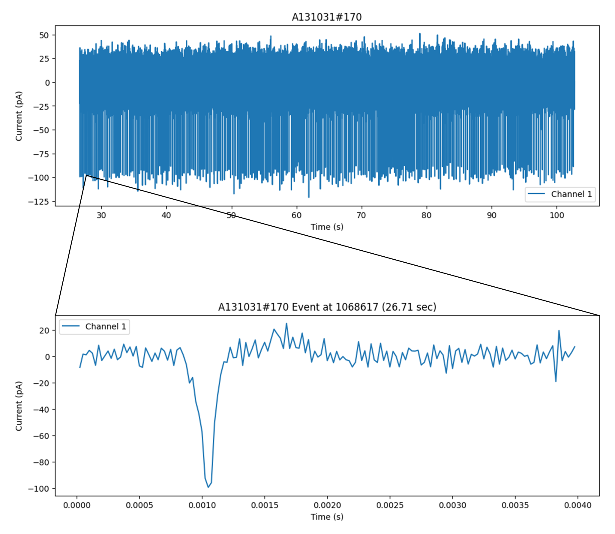
Figure 2: Example on how single events were isolated and selected. The image depicts the recording of the serotonergic cell A131031#170 and the 4 ms event of triggered at point 1068617, i.e. at 26.715 sec.

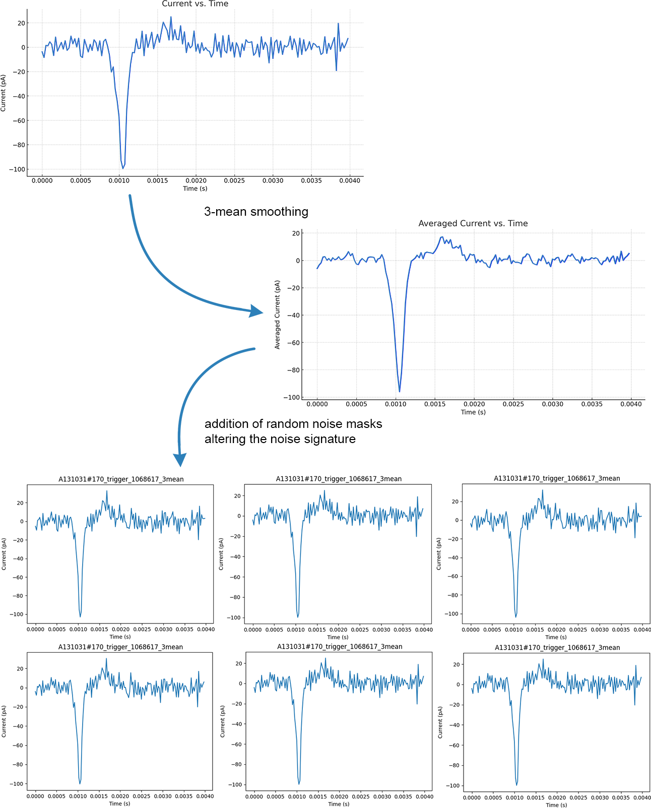
Figure 3: Example of 4 synthetic spikes generated by the event triggered at 1068617, i.e. 26.715 sec, of the serotonergic cell A131031#170. Top trace: the original recording of the event. The panels report four spike obtained by processing the original trace with different noise masks (see methods).

4 Generation of Synthetic Data

The use of synthetic data for deep learning models is increasingly important nowadays, more so in this case due to the lack of a large amount of collected data and the difficulty of experiments. In the generation of synthetic data for emulating spike recordings of serotonergic cells, some elements are important: firstly, it is paramount to maintain a spike waveform resulting from a depolarization and repolarization of the cell consistent with the biological ones; secondly, it is necessary to avoid imposing a spike morphology that is too uniform and which does not take into account the biological variability of individual cells; finally, it is desirable for the signal to contain a plausible but original and variable noise signature in order to have less sensitive trained models. The following procedure for generating synthetic data is developed in order to meet all the previous requirements. Note that not all requirements point toward the same operational direction. Indeed, one could think of eliminate from all spikes the background noise averaging all events (as it is often used for visual discrimination of serotonergic cells) thus obtaining a theoretical and ideal spike waveform that one would eventually combine with an ad hoc background noise. That would be an interesting solution that would, nevertheless compress the biological variability of a cell to a single action potential waveform. On the other hand, one might want to change arbitrarly the noise background in order to have very different signatures, but at the same time the unsupervised application of an arbitrary noise mask would yield in altering too substantially the spike waveform leading to unrealistic action potentials.

In our synthetic data generation procedure (Fig. 3), each original training data sample, i.e., each single event, is smoothed through a simple moving average (SMA) of range 3. The reason for using a SMA of range 3 is due to the need to combine two requirements: the need to smooth the original signal from the specific noise of the recording (for which SMA are a common technique), and the need to maintain the structure of the signal as mentioned above. Indeed, the rapid depolarization of the cell is such that the most relevant data of the spike recording are often condensed in about a dozen of recording points. This means that considering a SMA with range $n>3$ could undermine the fundamental information inside the signal, while $n=2$ might not be sufficient to remove the background noise. A visual inspection of the averaged signal in 3 shows that the bottom of the event is not altered by applying an SMA of range 3, while a higher ranged SMA could create a smooth bottom instead of a spike. Concretely, supposing a $4$ ms sample recorded at 40 kHz, the values of the smoothed sample $\left\{y^{\prime}_{m}\right\}$ with $m\in\left\{1,...,160\right\}$ are given as the averages of the values of the original sample $\left\{y_{m}\right\}$ by

$$\begin{cases}y^{\prime}_{1}=\frac{\left(y_{1}+y_{2}\right)}{2},\\ y^{\prime}_{m}=\frac{\left(y_{m-1}+y{}_{m}+y{}_{m+1}\right)}{3},&1<m<160\\ y^{\prime}_{160}=\frac{\left(y_{159}+y_{160}\right)}{2}.\end{cases}$$ (1)

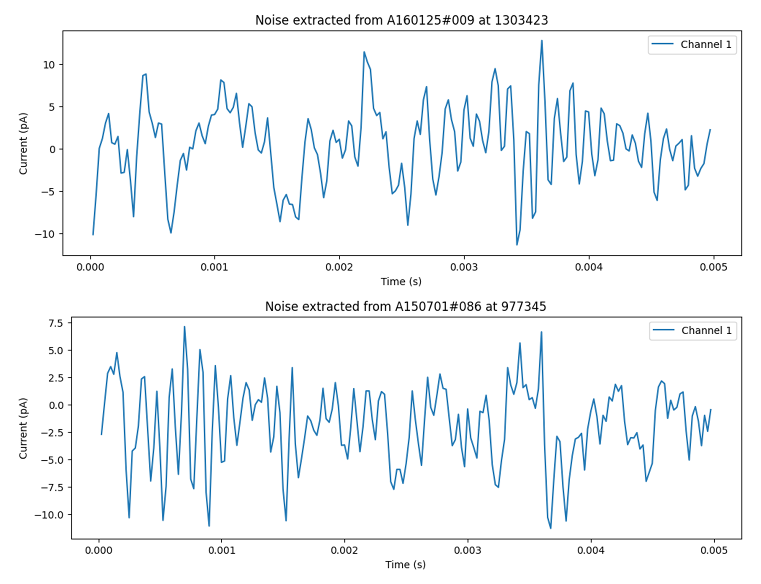
Figure 4: Examples of noise masks collected from the recordings of cell A160125#009 (on top) and A150701#086 (on bottom).

After the previous process has taken place, one has to recombine the averaged signal $\left\{y^{\prime}_{m}\right\}$ with a set of noise masks $\left\{n_{m}^{(k)}\right\}$ previously extracted (Fig. 4). From a practical standpoint, a good way to select such masks is to proceed with an extraction from real recordings of experiments performed on different days and under different environmental conditions. A noise mask is selected extracting a segment immediately before the trigger of an event, e.g., the noise recording from 5.5 ms to 2.5 ms before the peak of an event. This ensures the mask contains only background noise patterns uncorrelated with spike waveform features. Extracting masks in this manner from multiple heterogeneous recordings provides a diverse noise set to add variability. Moreover, considering it is quite feasible to obtain more than $10$ days of recordings, then selecting just 100 noise masks from each day would yield a 1000-fold increase in data augmentation through synthetic data generation. Indeed, combining $k=1000$ heterogeneous noise masks enables synthesizing 1000 distinct versions of each averaged spike. For computational and practical reasons, the augmentation multiplication factor $R$ is typically constrained to be considerably smaller than $k=1000$. Nevertheless, the authors suggest creating a noise mask pool with at least 1000 elements. Then for each original spike, randomly select $R$ masks from this large pool to generate the synthetic augmented samples. This approach helps ensure diversity and minimize correlations in the applied noise patterns.

The generation of $R$ synthetic data is then obtained from the values of smoothed spike $\left\{y^{\prime}_{m}\right\}$, that are then added to the values of $R$ randomly chosen noise mask $\left\{n_{m}^{(j)}\right\}$ where $j\in\left\{1,...,1000\right\}$ is randomly chosen. The final synthetic sample is thus obtained as the sample $\left\{y^{(j)}{}_{m}\right\}_{j\in\left\{1...R\right\}}$ with

$$y^{(j)}{}_{m}=y^{\prime}_{m}+\alpha\cdot n_{m}^{(j)},$$ (2)

where $\alpha\in\left[0.2,0.4\right]$ is a randomly generated “dumping coefficient” experimentally found around $0.3$ to modulate the noise. The choice of this coefficient requires some clarification. Indeed, the coefficient dumps the noise intensity to synthesize more physiologically plausible spike waveforms. First, the background noise was not completely removed when averaging spikes, just smoothed with a 3-point average. Thus directly adding the full noise mask would excessively boost the background noise compared to the original recording. Moreover, the original noise does not influence all points of the signal equally, but is more pronounced in slower changing current regions. Applying the raw noise mask tends to produce unrealistic spike shapes, e.g. double bottoms. The dumping coefficient $\text{rand}(0.2,0.4)$ was deemed a suitable range by visual inspections by an expert author with over 30 years of experience on serotonergic spike recordings.

5 A Practical Case

As a practical application of the previous procedure is given by the model for serotonergic cell recognition now available on GitHub at github.com/ neuraldl/ DLAtypicalSerotoninergicCells.git . To implement the model the authors used the following

Original Training Data:

The original training data for the training, validation and testing of the models consisted in 43,327 spike samples extracted from 108 serotonergic cells and 45 non-serotonergic cells. More specifically, the authors extracted 29,773 spikes from serotonergic cells, and 13,554 spikes from non-serotonergic cells. In all cases, the triggering threshold of the event was -50 pA and the spike was then sampled 1 ms before the triggering threshold until 3 ms after (see Fig. 1). Since the sampling rate of the original recordings was 40 kHz, every spike sample consists of 160 values.

Non-homogenous Data:

The non-homogenous data consisted in 24,616 samples extracted from 55 serotonergic cells and 27 non-serotonergic cells collected in experimental days not used to obtain the training data, thus with different noise signature. Again, the triggering threshold of the event was -50 pA and the spike was then sampled 1 ms before the triggering threshold until 3 ms after, yielding to 18595 spikes from serotonergic cells and 6021 from non-serotonergic cells. These data were never part of the training set, nor validation, nor testing set during the training, and constituted just an additional independent test for the already trained model.

Synthetic Data:

The synthetic data consisted in 12,700,600 spike samples of 160 points (simulating 4 ms at 40 kHz of sampling) arising from the 43327 original training data samples. From the original training data recordings the authors extracted 600 noise masks that constituted the pool for the random noise selection for obtaining the synthetic data.

The Architecture of the Neural Network:

Identifying serotonergic cells is a binary classification task, where cells are categorized as either serotonergic or non-serotonergic. Convolutional neural networks (CNNs) have demonstrated remarkable performance in this domain. Inspired by the structure of the animal visual system, particularly the human brain, CNNs excel at image feature extraction, a crucial aspect of recognition tasks (Liu, 2018). These networks utilize techniques such as feedforward inhibition to mitigate problems like gradient vanishing, thereby enhancing their performance in complex pattern recognition challenges (Liu et al., 2019).

Considering these advantages, the authors opted for a CNN architecture for the somewhat atypical application of numerical pattern recognition, specifically for analyzing the electrical signals from neuronal cells. This architecture comprises a series of layers typical in image recognition with deep learning using CNNs. The implementation was carried out using the Keras library within TensorFlow 2.15. The network includes a normalization layer to stabilize learning and expedite training, two sets of a 2D convolutional layer with 32 filters each, followed by a max pooling layer with a pool size of (2x1). It also features a flatten layer that connects to a dropout layer and subsequently to dense layers, which have two output units for the binary classification task. The activation function for the convolutional layers is ReLU, while the dense layers utilize the sigmoid function, detailed in Table 1. For training, the authors employed the ’binary crossentropy’ loss function, a standard in binary classification tasks, and ’Adam’ (Adaptive Moment Estimation) as the optimizer, given its widespread use and effectiveness.

Layer (type)	Output Shape	Param #
Layer Normalization	(None, 160, 2, 1)	320
Conv2D	(None, 141, 2, 32)	672
MaxPooling2D	(None, 70, 2, 32)	0
Conv2D	(None, 51, 2, 64)	41024
MaxPooling2D	(None, 25, 1, 64)	0
Flatten	(None, 1600)	0
Dropout	(None, 1600)	0
Dense	(None, 2)	3202
Total Params	45218

Table 1: Schematic of the neural network used with kernel 20. All other models follow the same architectural structure and change only for the dimension of the kernel. The final prediction is given by the consensus of the models with kernel from 20 through 30.

A special treatment was devoted to the kernel of the 2D convolutional layers. Indeed, since the kernel of these layers express the ability of the convolutional process in enlarging a specific portion of the pattern, the authors explored a range of possible kernels between 1 to 31. The training involving > 12M spike samples required a continuous learning implementation, where the model was trained over 200 training sessions of 63450 synthetic spike samples. More specifically, for each one of the 200 training sessions the 63450 synthetic spike samples (33.350 serotonergic and 30.100 non-serotonergic) the authors considered 44.415 spike for the effective training, 9.517 spike for validation and 9.518 for test. In each session, all models were trained on 25 epochs with a batch size of 64.

To enhance the robustness of the model, instead of selecting a single kernel and using one model for inference, the authors selected all models with kernels ranging between 20 and 30 and took the consensus between the models. This technique ensures more stability in the overall architecture and is often considered best practice.

Results on Test Data

Being trained over 12M spikes, i.e. 6,675,300 from serotonergic spikes and 6,025,300 originated from non-serotonergic spikes, the resulting model has impressive metrics on the test data. More specifically, the best training session has a test loss of $1,83\cdot 10^{-6}$, accuracy of $1$, sensitivity at specificity 0.5 of 1, 0 False Positive and 0 False Negative. However, these results are not deemed significant, as overfitting not related to recording noise tends to be amplified in the augmented dataset.

Results on Non-Homogenous Data

The most significant outcomes are on non-homogeneous data, i.e., cells that were not utilized in training and were collected on different days than the training data. Using this dataset, the synthetic model achieved an accuracy of 0.9375, a sensitivity at specificity 0.5 of 0.8888, an AUC of 0.9255 and an F1-Score of 0.9056. Even though later sessions have all similar metrics, the best training session was achieved in session 89 with the following metrics non-homogenous data (also results on the biological model on the same dataset are reported for comparison).

Model	Accuracy	Sens. at Spec. 0.5	AUC	F1-Score
Biological model	0.9125	0.8518	0.8976	0.8679
Synthetic model	0.9375	0.8888	0.9255	0.9056

A crucial indicator of performance is the model’s confusion matrix specifically a 96.2% True Positive Rate, 3.7% False Negative Rate; 88.8% True Negative Rate, and 11.1% False Positive Rate.

6 Conlusion and Discussion

This paper presented a methodology for generating synthetic spike data to train deep learning models in identifying typical and atypical serotonergic neurons using smoothed real spike waveforms with diverse noise masks extracted from different real experiments. A practical case study demonstrated the effectiveness of the method, with a CNN model trained on the augmented dataset achieving high accuracy on non-homogeneous test data. While synthetic data have proven effective, the approach may have limitations in fully capturing the diversity of real spiking patterns. Indeed, a special care must be taken during waveform smoothing and noise intensity calibration to preserve key features and avoid creating unrealistic spikes. Moreover it is important to stress out that the method was developed and validated for serotonergic neurons in mice, and its applicability to other species and cell types might require further investigation. Despite these limitations, the proposed approach enables the development of robust serotonergic neuron classifiers and opens up to future research (one would like to investigate advanced generative models like GANs and adaptive augmentation strategies). As experimental methods advance and more diverse serotonergic neuron datasets become available, the presented approach can be refined and extended.

References

Calizo, L. H.; Akanwa, A.; Ma, X.; Pan, Y.; Lemos, J. C.; Craige, C.; Heemstra, L. A.; Beck, S. G. Raphe Serotonin Neurons Are Not Homogenous: Electrophysiological, Morphological and Neurochemical Evidence. Neuropharmacology 2011, 61 (3), 524−543.

Corradetti, D.; Bernardi, A.; Corradetti R.; Deep Learning Models for Atypical Serotoninergic Cells Recognition. bioRxiv 2024.03.03.583157; doi: https://doi.org/10.1101/2024.03.03.583157

Hajós, M., Gartside, S.E., Villa, A.E., Sharp, T., 1995. Evidence for a repetitive (burst) firing pattern in a sub-population of 5- hydroxytryptamine neurons in the dorsal and median raphe nuclei of the rat. Neuroscience 69(1):189-97. doi:10.1016/0306- 4522(95)00227-a.

Mlinar B., Montalbano A., Piszczek L., Gross C., Corradetti R. (2016). Firing properties of genetically identified dorsal raphe serotonergic neurons in brain slices. Front. Cell Neurosci. 10:195. 10.3389/fncel.2016.00195

Montalbano, A., Waider,J., Barbieri,M., Baytas,O., Lesch,K.P., Corradetti,R., et al (2015). Cellular resilience: 5-HT neurons in Tph2 (-/-) mice retain normal firing behaviour despite the lack of brain 5-HT. Eur. Neuropsychopharmacol. 25, 2022–2035. doi:10.1016/j.euroneuro.2015.08.021

Okaty BW, Commons KG, Dymecki SM. 2019 Embracing diversity in the 5-HT neuronal system. Nat Rev Neurosci. 2019 20(7):397-424. doi: 10.1038/s41583-019-0151-3

Liu, Y. (2018). Feature Extraction and Image Recognition with Convolutional Neural Networks. Journal of Physics: Conference Series, 1087. https://doi.org/10.1088/1742-6596/1087/6/062032.

Liu, L., Yang, S., & Shi, D. (2019). Advanced Convolutional Neural Network With Feedforward Inhibition. 2019 International Conference on Machine Learning and Cybernetics (ICMLC), 1-5.

Vandermaelen, CP., & Aghajanian,G.K. (1983). Electrophysiological and pharmacological characterization of serotonergic dorsal raphe neurons recorded extracellularly andintracellularly in rat brain slices. Brain Res. 289, 109–119. doi:10.1016/0006-8993(83)90011-2.