Chiral dynamics with giant systems

Abstract

We explore the chiral dynamics in a parity-time-symmetric system consisting of a giant Kerr cavity nonlocally coupled to a one-dimensional waveguide. By tuning the phase difference between the two coupling points to match the propagation phase at the driving frequency, chiral cavity-waveguide interactions are achieved, enabling the deterministic generation of photons with nontrivial statistics only for a single incident direction. This nontrivial-statistical photons can be produced even in the strong dissipation regime due to the interference between reflected and transmitted photons propagating between the coupling points. Our investigation encompasses a broad range of distances between the coupling points, incorporating non-Markovian effects. Notably, at a phase difference of $\pi/2$, the system’s dynamics become exactly Markovian, while the output field retains non-Markovian characteristics. Under these conditions, we analyze nonreciprocal dissipative phase transitions driven by a strong external field and elucidate the influence of the non-Markovian effect. Our results offer valuable insights for the advancement of nonreciprocal photon devices and deterministic photon generations, providing a deeper understanding of dissipative phase transitions.

The precise control of single-photon-level light-matter interactions in confined structures is pivotal for advancing both fundamental quantum research and practical applications, such as the generation of cat states and the development of quantum communication systems Milonni (2013); Kimble (1998); Walls and Milburn (2008); Haroche and Raimond (2006). Over recent decades, chiral quantum optics, which involves the direction-dependent coupling between an emitter and light propagating in a one-dimensional medium, has garnered significant attention Gardiner (1993); Carmichael (1993); Soro and Kockum (2022); Lodahl et al. (2017); Roushan et al. (2017); Kannan et al. (2023). This interaction framework opens up avenues for creating novel quantum many-body states Stannigel et al. (2012); Ramos et al. (2014) and developing cascaded quantum networks Cirac et al. (1997); Kimble (2008).

Initial implementations of chiral interactions utilized nanophotonic devices, where confined photons of different polarizations propagate in opposite directions Petersen et al. (2014); Sayrin et al. (2015); Scheucher et al. (2016); Lodahl et al. (2017). In these systems, transitions between certain emitter states can be induced exclusively by light traveling in a specific direction. To enhance control over the interaction strength and mitigate unwanted environmental interactions, recent experimental advances have demonstrated the use of chiral artificial atoms based on superconducting-circuit platforms Joshi et al. (2023). The core innovation in these systems is the concept of the giant atom Frisk Kockum et al. (2014); Guo et al. (2017); Kockum et al. (2018); Kannan et al. (2020); Soro and Kockum (2022); Cheng et al. (2022); Noachtar et al. (2022); Terradas-Briansó et al. (2022), which couples to multiple points along a transmission line. Using state-of-the-art techniques McKay et al. (2016); Roushan et al. (2017); Yan et al. (2018); Joshi et al. (2023), the relative phase $\varphi$ between these nonlocal coupling points can be precisely adjusted, thereby breaking parity symmetry and inducing chirality in the single-photon scattering spectrum.

Previous studies on chirality in giant systems in the non-Markovian regime have predominantly concentrated on single-excitation scenarios Guimond et al. (2020); Wang et al. (2021); Chen et al. (2022); Cheng et al. (2022); Wang and Li (2022); Roccati and Cilluffo (2024), where nonlinear effects do not play a role. In this letter, we investigate the chiral dynamics of a driven giant system incorporating its nonlinearity and the retardation effect Shi et al. (2015). We demonstrate that for a nonzero phase $\varphi$, photons input from one direction with a matched propagation phase do not interact with the giant system Joshi et al. (2023), resulting in coherent light in the transmission. Conversely, when driven from the opposite direction, the transmitted photons exhibit nontrivial statistical properties. In the weak-driving regime, this deterministic generation of beyond-Poissonian photons is enabled by the system’s parity-time ($\mathcal{PT}$) symmetry, with the statistical characteristics governed by the nonlinearity. Remarkably, even in the strong dissipation limit where the nonlinearity is significantly smaller than the decay rate, nontrivial photon statistics emerge due to the interference of photons propagating between the nonlocal coupling points.

We study the nonreciprocal second-order coherence of transmitted photons, incorporating the prominent non-Markovian characteristic of giant systems Shi et al. (2015). Remarkably, for phase differences of $\varphi=\pm\pi/2$, interference between the two coupling points vanishes, simplifying the system’s dynamics to be exactly Markovian. In this scenario, the system can be precisely described using a master equation Gardiner and Zoller (2004); Walls and Milburn (2008) and a nonlocal input-output formalism, enabling the exact determination of its evolution under driving fields of arbitrary strength. Consequently, this framework offers a compelling platform for the realization of nonreciprocal dissipative phase transitions (DPTs) Houck et al. (2012); Kessler et al. (2012); Diehl et al. (2008); Carmichael (2015); Fitzpatrick et al. (2017); Aspelmeyer et al. (2014); Benito et al. (2016); Minganti et al. (2018) and the exploration of non-Markovian effects in such transitions. By leveraging the giant system’s tunable phase and the resulted coherence properties, we advance the understanding of nonreciprocal quantum dynamics and provide a pathway for novel quantum state engineering and control.

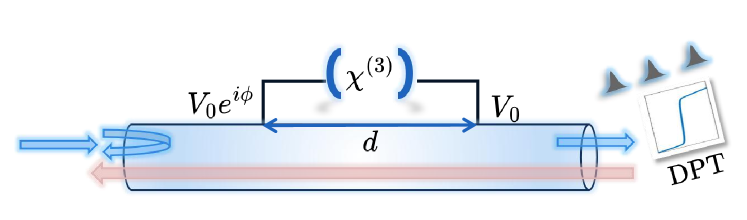
Figure 1: Schematic of a giant Kerr cavity coupled to a waveguide at two coupling points separated by a distance $d$. The coupling phase $\varphi$ can be tuned to a nonzero value, breaking parity symmetry. When the propagation phase at the driving frequency matches $\varphi$, the giant system interacts only with the right-moving driving field (indicated by the right arrow), which is either reflected or transmitted, while it remains transparent to the left-moving input (indicated by the red arrow). In the former case, the transmitted light reveals novel characteristics, such as nontrivial statistical behaviors and the occurrence of dissipative phase transitions (DPTs).

We use a giant Kerr cavity, which reduces to a giant two-level atom as its nonlinearity $U$ approaches infinity, as a paradigmatic example to demonstrate chiral dynamics. The setup, illustrated in Fig. 1, involves a giant Kerr cavity nonlocally coupled to a 1D bath (the waveguide) at two points, $0$ and $d$. Without loss of generality, we introduce a phase shift $\varphi$ at coupling point $0$, as only the phase difference between the two coupling points is relevant. The full Hamiltonian $H=H_{0}+H_{1}$, where

$$H_{0}=\frac{U}{2}b^{{\dagger}2}b^{2}+H_{D}+\sum_{\lambda=L,R}\int_{-\infty}^{+\infty}\varepsilon_{\lambda k}a_{\lambda k}^{{\dagger}}a_{\lambda k}\mathrm{d}k,$$ (1)

is the free Hamiltonian of the cavity and the waveguide respectively, plus the driving term $H_{\lambda D}=\left(\Omega_{\lambda}\left(k_{i}\right)b^{\dagger}e^{-i\varepsilon_{\lambda k_{i}}t}+H.c.\right)$, where $b$ ($a_{\lambda k}$) is the annihilation operator for the cavity mode ($\lambda$-moving bath mode with momentum $k$), and their interaction is depicted by

$$H_{1}=\sum_{\lambda=L,R}\int_{-\infty}^{+\infty}V_{\lambda k}a_{\lambda k}b^{{\dagger}}\mathrm{d}k+\mathrm{H.c..}$$ (2)

Here, $\Omega_{\lambda}\left(k_{i}\right)=\Omega_{0}\eta_{\lambda k_{i}}\left(\phi\right)$ is the Rabi frequency of the driving field propagating in direction $\lambda$ with momentum $k_{i}$, where $\Omega_{0}$ is a constant strength, and $\eta_{\lambda k_{i}}\left(\phi\right)=e^{i\phi}+e^{i\theta_{\lambda k_{i}}}$, with the propagation phase $\theta_{\lambda k_{i}}=\left(\sigma_{\lambda}k_{0}+k_{i}\right)d$, $\sigma_{R}=1$, and $\sigma_{L}=-1$. $k_{0}$ is the central frequency of the bath, assumed to be the same as the cavity frequency. The $k$-dependent coupling strength $V_{\lambda k}=V_{0}\eta_{\lambda k}\left(\phi\right)$, where $V_{0}$ is a constant strength. The spectrum of the bath is assumed to be linear, i.e., $\varepsilon_{\lambda k}=\sigma_{\lambda}k$, but it can be extended to other spectra, such as cosine spectrum Chang et al. (2011); Shi et al. (2016) and Ohmic spectrum Shi et al. (2018).

By tuning the phase $\phi$ to match the propagation phase at a driving frequency $k_{i}$, corresponding to $\Omega_{L}\left(-k_{i}\right)$ and $\Omega_{R}\left(k_{i}\right)$, the giant system can be selectively decoupled from either the left- or right-moving driving field, effectively realizing the chiral light-emitter interaction. Additionally, reversing the direction of the input photons is equivalent to changing $\phi$ to $-\phi$. Without loss of generality, in the following, we focus on the case with

$$\phi=\left(2n+1\right)\pi-\left(k_{0}+k_{i}\right)d,$$ (3)

which results in $\Omega_{L}\left(-k_{i}\right)=0$, where $n$ is an integer, and study the chiral dynamics for right-moving inputs with frequency $k_{i}$.

In the weak-driving limit, the dynamics are governed by the lowest-order behavior of $\Omega_{0}$ and can be linked to few-photon scattering processes Shi et al. (2015); Chang et al. (2016). For instance, reflection and transmission probabilities can be acquired by calculating the single-photon scattering processes, while second-order coherence can be inferred from the two-photon wavefunction. In the case of single-photon scattering, the reflection is reciprocal due to the parity-time ($\mathcal{PT}$) symmetry Sakurai and Napolitano (2020) of the system. Namely, the reflection coefficients satisfy $\left\langle 0\right|a_{Rk}Sa_{L-k_{i}}^{\dagger}\left|0\right\rangle=\left\langle 0\right|a_{L-k}Sa_{Rk_{i}}^{\dagger}\left|0\right\rangle$, where $|0\rangle$ is the vacuum state and the $S$ matrix is defined as $S=\lim_{T\rightarrow+\infty}^{\Omega_{0}\rightarrow 0}e^{iH_{0}T}e^{-i2HT}e^{iH_{0}T}$ Sakurai and Napolitano (2020). Consequently, the transmission probabilities for single left-moving and right-moving input photons are identical. Utilizing the method developed in Shi et al. (2015), where the bath field is integrated out via a path integral approach, we obtain the self-energy Fetter and Walecka (2012); Shi et al. (2016) $\Sigma(\omega)\equiv\sum_{\lambda=L,R}\int\frac{|V_{\lambda k}|^{2},\mathrm{d}k}{\omega-\varepsilon_{\lambda k}+i0^{+}}$ as

$$\Sigma\left(k\right)=-i2\gamma\left(1+\cos\phi e^{i\theta_{Rk}}\right),$$ (4)

where $\gamma=2\pi V_{0}^{2}$ is the decay rate accounting for cavity-bath coupling at a single point. Consequently, the reflection and transmission coefficients with input and output momenta $k_{i}$ and $k_{f}$, can be written as sup $\left\langle 0\right|a_{Lk_{f}}Sa_{Rk_{i}}^{\dagger}\left|0\right\rangle=r\left(k_{i}\right)\delta\left(k_{i}+k_{f}\right)$ and $\left\langle 0\right|a_{Rk_{f}}Sa_{Rk_{i}}^{\dagger}\left|0\right\rangle=t\left(k_{i}\right)\delta\left(k_{i}-k_{f}\right)$, where

$$r\left(k\right)=-i\gamma\eta_{L-k}^{\ast}\left(\phi\right)G\left(k\right)\eta_{Rk}\left(\phi\right)$$ (5)

and

$$t\left(k\right)=1-i\gamma\left|\eta_{Rk}\left(\phi\right)\right|^{2}G\left(k\right),$$ (6)

with the Green function Fetter and Walecka (2012); Shi et al. (2015, 2016) $G\left(k\right)=\left[k-\Sigma\left(k\right)\right]^{-1}$.

Under the condition given by Eq. (3), the $\mathcal{PT}$ symmetry of the system ensures that the transmission probability for single right-moving photons is unity, indicating deterministic photon generation in the transmitted direction for both input orientations. However, the statistical properties of the right-moving transmitted photons can markedly differ from the trivial one for those ones moving to the left. Specifically, for two input photons with identical momentum $k_{i}$, the $S$-matrix element $S_{p_{2}p_{1},k_{i}k_{i}}\equiv\left\langle 0\right|a_{Rp_{2}}a_{Rp_{1}}Sa_{Rk_{i}}^{\dagger}a_{Rk_{i}}^{\dagger}\left|0\right\rangle$ governing the transmission of two photons with momenta $p_{1}$ and $p_{2}$ is sup

$$S_{p_{2}p_{1},k_{i}k_{i}} = 2t\left(k_{1}\right)t\left(k_{2}\right)\delta\left(k_{i}-p_{1}\right)\delta\left(k_{i}-p_{2}\right)$$ (7)

$$-i\Gamma_{p_{2}p_{1},k_{i}k_{i}}\left(\phi\right)\delta\left(2k_{i}-p_{1}-p_{2}\right)$$

where $\Gamma_{p_{2}p_{1},k_{i}k_{i}}=\frac{\gamma^{2}}{\pi}\eta_{Rp_{2}}^{\ast}\eta_{Rp_{1}}^{\ast}G\left(p_{1}\right)G\left(p_{2}\right)T_{S}G^{2}\left(k_{i}\right)\eta_{Rk_{i}}^{2}$ and

$$T_{S}=\frac{U}{1-\frac{U}{k_{i}+i2\gamma}\sum_{mn}F_{mn}\left(k_{i}\right)\Theta\left(m-n\right)}$$ (8)

depends on the input momentum $k_{i}$. The function $F_{mn}\left(k\right)=\frac{e^{i\left(m-n\right)\left(k+i2\gamma\right)d}}{m!}\left(\frac{-i\gamma\cos\phi e^{i\theta_{Rk}}}{k+i2\gamma}\right)^{m+n}\sum_{l=0}^{n}C_{mnl}\left(k\right)$, with $C_{mnl}\left(k\right)=\frac{\left(m+n-l\right)!}{\left(n-l\right)!l!}\left[-i2\left(m-n\right)\left(k+i2\gamma\right)d\right]^{l}$. In Eq. (7), the first term is resulted from the independent scattering of the two photons, while the second term represents the background fluorescence Shen and Fan (2007); Shi and Sun (2009).

The second-order correlation function $g_{\lambda}^{\left(2\right)}\left(\tau\right)\equiv\frac{\left\langle a_{out}^{\lambda\dagger}\left(0\right)a_{out}^{\lambda\dagger}\left(\tau\right)a_{out}^{\lambda}\left(\tau\right)a_{out}^{\lambda}\left(0\right)\right\rangle}{\left\langle a_{out}^{\lambda\dagger}\left(0\right)a_{out}^{\lambda}\left(0\right)\right\rangle^{2}}$, where the output fields $a_{out}^{\lambda}\left(t\right)=\frac{1}{\sqrt{2\pi}}\int a_{\lambda k}\left(T\right)e^{-i\sigma_{\lambda}k\left(t-T\right)}\mathrm{d}k$, is connected to the two-photon wavefunction $w_{\lambda}\left(X_{1},X_{2}\right)$ with two photons at positions $X_{1}$ and $X_{2}$ as $g_{\lambda}^{\left(2\right)}\left(\tau\right)=\left|\frac{w_{\lambda}\left(\tau,0\right)}{w_{\lambda}\left(\tau\rightarrow\infty,0\right)}\right|^{2}$, while the wavefunction $w_{t}\left(X_{1},X_{2}\right)$ of two transmitted photons can be acquired by performing the Fourier transform of $S_{p_{2}p_{1},k_{2}k_{1}}$ as

$$w_{t}\left(X_{1},X_{2}\right)=\frac{1}{2\pi}\int dp_{1}dp_{2}e^{ip_{1}X_{1}}e^{ip_{2}X_{2}}S_{p_{2}p_{1},k_{2}k_{1}}.$$ (9)

By fixing $\theta_{Rk_{i}}=\pi-\varphi$, we investigate the statistics of transmitted photons for right-moving inputs, varying both $k_{i}$ and $\varphi$. The results are depicted in Fig. 2. When $U$ is comparable to the decay rate $\gamma$, the output photons can exhibit sub-Poissonian ($g_{R}^{(2)}(0)<1$) or super-Poissonian ($g_{R}^{(2)}(0)>1$) statistics for input momenta $k_{i}$ within a width approximately $\gamma$. In contrast to the single-point coupling scenario Shi et al. (2011), nontrivial statistical behaviors of transmitted photons persist even in the strong dissipation regime where $\gamma\gg U$, as shown in Fig. 2(b). Further tuning of $k_{i}$ and $\varphi$ reveals that the second-order correlation function $g_{R}^{(2)}(0)$ varies in a wide range from $10^{-2}$ to $10^{4}$ (Fig. 2(c)). This nontrivial statistical behavior arises from photon interference between the two coupling points, resulting in an effective decay rate $-\text{Im}[\Sigma(k)]=2\gamma[1+\cos\varphi\cos\theta_{Rk}]$ for the $k$-th mode, which can be significantly smaller than $U$. These modes can be excited in the two-photon scattering process by matching the input momentum $k_{i}$ with the real part of the its self-energy, $\text{Re}[\Sigma(k)]=2\gamma\cos\varphi\sin\theta_{k}$. Fig. 2(d) illustrates this phenomenon with the background fluorescence Shen and Fan (2007); Shi and Sun (2009) $\Gamma_{p_{2}p_{1},k_{i}k_{i}}$ at the point indicated by the rectangle in Fig. 2(c), where $k_{i}=0.09\gamma$, $\varphi=0.015\pi$, and $g_{R}^{(2)}(0)=0.017$, corresponding to $\Sigma(k_{i})=(0.094-i0.0044)\gamma$. Fig. 2(d) shows highly populated modes centered at $k_{i}+n\frac{2\pi}{d}$ with a narrow width of $-$Im$[\Sigma(k)]/\left(\gamma L\right)$, underscoring the nontrivial statistical behaviors of transmitted photons.

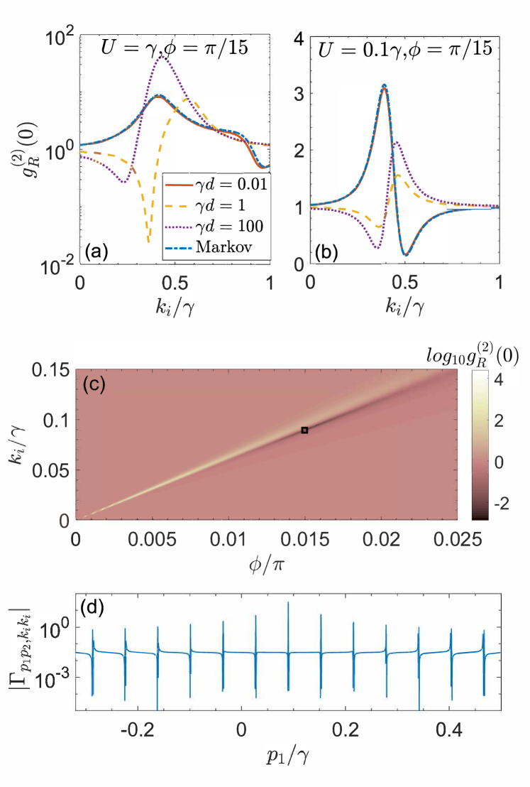
Figure 2: Properties of the output photons in the weak-driving limit. (a) Second-order correlation function $g_{R}^{(2)}(0)$ of the transmitted light with $\phi=\pi/15$ and $U=\gamma$. (b) Same as (a), but for weak nonlinearity $U=0.1\gamma$. (c) $g_{R}^{(2)}(0)$ as a function of $k_{i}$ and $\phi$ in the strong dissipation limit with $U=0.01\gamma$. (d) Background fluorescence $\left|\Gamma_{p_{2}p_{1},k_{i}k_{i}}\right|$ with parameters from the rectangle in (c). Here, in $\Gamma_{p_{2}p_{1},k_{i}k_{i}}$, $p_{2}=2k_{i}-p_{1}$.

When $\gamma d\ll 1$, the two-photon process simplifies to be Markovian (dashed-dotted line in Figs. 2(a) and (b)), and the system’s evolution can be approximatly described by a master equation and the input-output formalism Gardiner and Zoller (2004); Walls and Milburn (2008). Generally, this Markovian approximation breaks down for large distances $d$, as evidenced by the deviation in the second-order correlator $g_{R}^{(2)}(0)$ between $\gamma d=0.01$ and $\gamma d=1,100$ (for fixed $\theta_{Rk_{i}}$, Markovian dynamics are independent of $d$). However, when $\phi=\pm\pi/2$, the self-energy $\Sigma(k)$ becomes independent of $k$, and the evolution of the giant cavity’s density matrix $\rho$ can be exactly described by the master equation Shi et al. (2015) regardless of the distance $d$ :

$$\partial_{t}\rho=-i\left[H_{S},\rho\right]+2\gamma\left(2b\rho b^{\dagger}-\left\{b^{\dagger}b,\rho\right\}\right),$$ (10)

where $\rho$ is the density matrix of the cavity and $H_{S}=\frac{U}{2}b^{{\dagger}2}b^{2}+H_{\lambda D}$. In this scenario, the decay of the cavity due to the interference between right- and left-moving photons propagating between the two coupling points is completely canceled out. This cancellation can also be understood by defining two modes

$$\left(\begin{array}[]{c}A_{+k}\\ A_{-k}\end{array}\right)=U_{k}\left(\begin{array}[]{c}a_{L-k}\\ a_{Rk}\end{array}\right),$$ (11)

where the unitary transformation $U_{k}=\frac{1}{\tilde{V}_{k}}\left(\begin{array}[]{cc}V_{L-k}&V_{Rk}\\ V_{Rk}^{\ast}&-V_{L-k}^{\ast}\end{array}\right)$, with $\tilde{V}_{k}=2V_{0}\sqrt{1+\cos\phi\cos\left(k_{0}+k\right)L}$. These two modes are degenerated and decoupled, and the cavity field only couples to $A_{+k}$ mode with the interaction in Eq. (2) rewritten as

$$H_{1}=\int_{-\infty}^{+\infty}\tilde{V}_{k}\left(b^{{\dagger}}A_{+k}+\mathrm{H.c.}\right)\mathrm{d}k\mathrm{.}$$ (12)

When $\phi=\pm\pi/2$, $\tilde{V}_{k}$ is independent of $k$, leading to a constant decay rate $2\gamma$ contributed from the incoherent superposition of cavity photons decaying via the two coupling points. Note that this $k$-independence in $\tilde{V}_{k}$ with $\phi=\pm\pi/2$ is general and does not depend on the specific spectrum $\varepsilon_{\lambda k}$. However, the Markovian description is rigorously valid only for a linear spectrum. Furthermore, the properties of photons propagating in the waveguide can be acquired with the input-output relation

$$a_{out}^{\lambda}\left(t\right)=a_{in}^{\lambda}\left(t\right)-i\sqrt{\gamma}\left[e^{-i\phi}b\left(t\right)+e^{-i\theta_{\lambda 0}}b\left(t+\sigma_{\lambda}d\right)\right],$$ (13)

where the input field $a_{in}^{\lambda}\left(t\right)=\frac{1}{\sqrt{2\pi}}\int a_{\lambda k}\left(0\right)e^{-i\sigma_{\lambda}kt}\mathrm{d}k$. Note that unlike the giant system itself, the output field $a_{out}^{\lambda}\left(t\right)$ is determined by the cavity field at two distinct times $t$ and $t\pm d$ even when $\phi=\pm\pi/2$. This indicates that the non-Markovian characteristic is preserved in the properties of the output photons.

The master equation (10), along with the input-output formalism (13), enables a comprehensive exploration of the giant system’s dynamics and the characteristics of the output photons under arbitrarily strong driving fields. When $\phi=(k_{0}+k_{i})d=\pi/2$, the giant system interacts exclusively with the right-moving driving field, leading to the emergence of a DPT in the strong-driving regime Drummond and Walls (1980); Drummond and Gardiner (1980); Bartolo et al. (2016). As depicted in Fig. 3(a), increasing the pump strength $\Omega_{0}$ results in a sudden increase in the cavity photon number $\langle b^{{\dagger}}b\rangle_{S}$ around $\Omega_{0}\approx 5\gamma$, corresponding to a peak in the second-order correlator $g^{(2)}(0)\equiv\frac{\langle b^{{\dagger}2}b^{2}\rangle_{S}}{\langle b^{{\dagger}}b\rangle_{S}^{2}}$, where $\langle...\rangle_{S}$ denotes the steady-state average. Here, we consider Kerr nonlinearity $U=\gamma$ and input momentum $k_{i}=10\gamma$. Using methods such as the complex P-representation formalism Walls and Milburn (2008); Drummond and Walls (1980); Drummond and Gardiner (1980); Bartolo et al. (2016) or the quantum absorber approach Stannigel et al. (2012); Roberts and Clerk (2020), one can analytically derive the steady-state solution of the master equation (10), revealing a first-order DPT in the thermodynamic limit where the Liouvillian gap (the real part of the second-largest eigenvalue of the Liouvillian) vanishes at the critical point Minganti et al. (2018). Remarkably, this DPT-induced sudden change manifests not only in the cavity field but also in the reflected field, highlighting the non-Markovian effects induced by the giant system. At $T\rightarrow\infty$, the density $\rho_{L}\equiv\frac{1}{2\pi}\int\langle a_{Lk_{2}}^{{\dagger}}(T)a_{Lk_{1}}(T)\rangle e^{i(k_{1}-k_{2})X}\mathrm{d}k_{1}\mathrm{d}k_{2}$ of left-moving output photons at position $X<0$ can be computed using the input-output relation (13) as

$$\rho_{L} = \left\langle a_{out}^{L{\dagger}}\left(T+x\right)a_{out}^{L}\left(T+x\right)\right\rangle$$ (14)

$$= 2\gamma\left(\left\langle b^{{\dagger}}b\right\rangle_{s}+\text{Im}\left[e^{-ik_{0}d}\left\langle b^{{\dagger}}\left(d\right)b\left(0\right)\right\rangle_{S}\right]\right).$$

The reflected photon density $\rho_{L}$ depends on the distance $d$ through the nonlocal correlation $\left\langle b^{{\dagger}}(d)b(0)\right\rangle_{S}$. To examine the impact of this two-point correlation, we set $k_{0}d=\pi/2$ and $d=2n\pi/k_{i}$ to satisfy the chirality condition in Eq. (3), and investigate the nonreciprocal dissipative phase transition (DPT) via $\rho_{L}$ for various $d$. When $d=0$, no photons are reflected, while a peak emerges around the critical point as $d$ increases, as illustrated in Fig. 3(b). This peak occurs near the critical point where the Liouvillian exhibits a minimal gap (note that this gap only vanishes in the limit of infinite photon numbers), leading to the maximum correlation $\left\langle b^{{\dagger}}(d)b(0)\right\rangle_{S}-\left|\left\langle b\right\rangle_{S}\right|^{2}$ (Fig. 3(b)). As $d$ further increases, the peak in $\rho_{L}$ approaches the critical point, and the magnitude of the correlator $\left\langle b^{{\dagger}}(d)b(0)\right\rangle_{S}-\left|\left\langle b\right\rangle_{S}\right|^{2}$ diminishes because only the eigenstate with the smallest gap contributes significantly. Specifically, when $d$ exceeds the Liouvillian gap significantly, such as $d=2000\pi/k_{i}$, represented by the dotted lines in Fig. 3(b), no correlations are present and $\left\langle b^{{\dagger}}(d)b(0)\right\rangle_{S}$ approaches $\left|\left\langle b\right\rangle_{S}\right|^{2}$. In this scenario, the photon density $\rho_{L}$ reaches its maximum since $\left\langle b^{{\dagger}}(d)b(0)\right\rangle_{S}$ deviates most significantly from $\left\langle b^{{\dagger}}b\right\rangle_{S}$. Therefore, this system provides a platform to investigate the nonlocal effects in the context of DPT.

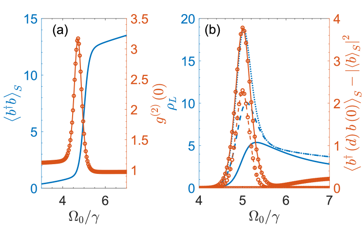
Figure 3: DPT occurs only when the giant system is driven by right-moving input. (a) Photon number (blue solid line, left axis) in the cavity and the second-order correlation function (red line with circles, right axis), as functions of the driving strength (b)Photon number density (blue lines, left axis) of the reflected field and the two-point correlation (red lines with circles, right axis). for different distance $\gamma d=0.63$ (solid lines), $\gamma d=63$ (dashed lines), and $\gamma d=6300$ (dotted lines). Other parameters are $U=\gamma$ and $k_{i}=10\gamma$.

In this work, we have investigated the dynamics of a driven giant system under chiral conditions, specifically when the phase difference $\phi$ between the two coupling points matches the propagation phase at the driving frequency. We focused on a giant cavity with nonlinearity $U$ that interacts solely with input light from a single direction. In the weak-driving regime, equivalent to a few-photon scattering process, we demonstrated that photons with nontrivial statistics can be deterministically generated, even in the strong dissipation regime where $U$ is small. This is due to the interference in the reflection and transmission of photons propagating between the two coupling points. Notably, when $\phi=\pm\pi/2$, this interference vanishes, resulting in Markovian dynamics for the giant system, while the reflected and transmitted light retains non-Markovian properties. In this scenario, we show that a nonreciprocal DPT can occur, and the density of reflected photons is influenced by nonlocal correlations. Our findings may inspire new applications and advancements in nonreciprocal photon devices and deterministic photon generation. Furthermore, we present a way to explore nonlocal correlations through photon reflection, offering fundamental insights into phenomena in the DPT .

Supplemental Materials

In this supplemental material, we show a detailed derivation of the single- and two-photon S matrix, using the method developed in Shi et al. (2015). First, we rewrite the $S$ matrix for reflection and transmission photons in forms of the two modes $A_{\pm k}$ defined in Eq. (11) as

$$\left(\begin{array}[]{c}A_{+k}\\ A_{-k}\end{array}\right)=U_{k}\left(\begin{array}[]{c}a_{L-k}\\ a_{Rk}\end{array}\right).$$ (S1)

Since only the modes $A_{+k}$ couple to the giant system, the transmission amplitude $\left\langle 0\right|a_{Rk_{f}}Sa_{Rk_{i}}^{\dagger}\left|0\right\rangle$ for a right-moving photon with input momentum $k_{i}$ and an output photon with momentum $k_{f}$ is

$$\left\langle 0\right|a_{Rk_{f}}Sa_{Rk_{i}}^{\dagger}\left|0\right\rangle = \left|U_{k_{i},22}\right|^{2}\delta\left(k_{i}-k_{f}\right)+\left|U_{k_{i},12}\right|^{2}\left\langle 0\right|A_{k_{f}+}SA_{k_{i}+}^{\dagger}\left|0\right\rangle$$ (S2)

$$= \left|U_{k_{i},22}\right|^{2}\delta\left(k_{i}-k_{f}\right)+\left|U_{k_{i},12}\right|^{2}\left\langle 0\right|A_{k_{f}+}e^{-i2HT}A_{k_{i}+}^{\dagger}\left|0\right\rangle e^{i\left(k_{i}+k_{f}\right)T},$$

where $T\rightarrow+\infty$. Similarly, the reflection amplitude

$$\left\langle 0\right|a_{Lk_{f}}Sa_{Rk_{i}}^{\dagger}\left|0\right\rangle=U_{-k_{f},21}^{\ast}U_{k_{i},22}\delta\left(k_{i}+k_{f}\right)+U_{-k_{f},11}^{\ast}U_{k_{i},12}\left\langle 0\right|A_{-k_{f}+}e^{-2HT}A_{k_{i}+}^{\dagger}\left|0\right\rangle e^{ik_{i}T}e^{-ik_{f}T}.$$ (S3)

For two photons, the amplitude for right-moving incident photons with momenta $k_{1}$ and $k_{2}$, and transmitted photons with momenta $p_{1}$ and $p_{2}$, is

$$\left\langle 0\right|a_{Rp_{1}}a_{Rp_{2}}Sa_{Rk_{2}}^{\dagger}a_{Rk_{1}}^{\dagger}\left|0\right\rangle$$ (S4)

$$= U_{p_{2},22}^{\ast}U_{p_{1},22}^{\ast}U_{k_{2},22}U_{k_{1},22}\left[\delta\left(k_{1}-p_{1}\right)\delta\left(k_{2}-p_{2}\right)+\left(k_{1}\longleftrightarrow k_{2}\right)\right]$$

$$+\{U_{p_{2},22}^{\ast}U_{p_{1},12}^{\ast}U_{k_{2},22}U_{k_{1},12}\left\langle 0\right|A_{p_{1}+}e^{-i2HT}A_{k_{1}+}^{\dagger}\left|0\right\rangle e^{i\left(k_{1}+p_{1}\right)T}\delta\left(k_{2}-p_{2}\right)$$

$$+\left(k_{1}\longleftrightarrow k_{2}\right)+\left(p_{1}\longleftrightarrow p_{2}\right)+\left(k_{1}\longleftrightarrow k_{2},p_{1}\longleftrightarrow p_{2}\right)\}$$

$$+U_{p_{2},12}^{\ast}U_{p_{1},12}^{\ast}U_{k_{2},12}U_{k_{1},12}\left\langle 0\right|A_{p_{2}+}A_{p_{1}+}e^{-i2HT}A_{k_{2}+}^{\dagger}A_{k_{1}+}^{\dagger}\left|0\right\rangle e^{i\left(k_{1}+k_{2}+p_{1}+p_{2}\right)T}.$$

Therefore, instead of the original left- and right-moving modes $a_{Lk}$ and $a_{L-k}$, we can obtain the S-matrix by considering only the $A_{k+}$ mode while the $A_{k-}$ mode is decoupled from the giant system. Here, we have assumed that in the initial and final states, the giant system is in vacuum, which is the case we focus on in the weak-driving limit.

I S-matrix in coherent-state presentation

To calculate the S-matrix ultilizing the path-integral method, we write it in the basis of coherent-states. The S-matrix for $N$ input photons with momenta $k_{i_{1}}k_{i_{2}},...,k_{i_{N}}$ and $N$ output photons with momenta $k_{f_{1}}k_{f_{2}},...,k_{f_{N}}$ envolves the calculation of

$$\left\langle k_{f_{1}}k_{f_{2}}...k_{f_{N}}\right|e^{-i2HT}\left|k_{i_{1}}k_{i_{2}}...k_{i_{N}}\right\rangle,$$ (S5)

where $\left|k_{1}k_{2}...k_{N}\right\rangle=A_{k_{N}+}^{\dagger}...A_{k_{2}+}^{\dagger}A_{k_{1}+}^{\dagger}\left|0\right\rangle$. Introducing an unnormalized coherent state Walls and Milburn (2008)

$$\left|\alpha_{k}\right\rangle=\sum_{n_{k}=0}\frac{\alpha_{k}^{n}}{\sqrt{n_{k}!}}\left|n_{k}\right\rangle,$$ (S6)

for the $k$-th mode $A_{k+}^{\dagger}$, the the evolution term $\left\langle k_{f_{1}}k_{f_{2}}...k_{f_{N}}\right|e^{-i2HT}\left|k_{i_{1}}k_{i_{2}}...k_{i_{N}}\right\rangle$ can be written as

$$\left\langle k_{f_{1}}k_{f_{2}}...k_{f_{N}}\right|e^{-i2HT}\left|k_{i_{1}}k_{i_{2}}...k_{i_{N}}\right\rangle$$ (S7)

$$= \lim_{\alpha_{k_{i_{1}}}\rightarrow 0}\partial_{\alpha_{k_{i_{1}}}}\lim_{\alpha_{k_{i_{2}}}\rightarrow 0}\partial_{\alpha_{k_{i_{2}}}}...\lim_{\alpha_{k_{i_{N}}}\rightarrow 0}\partial_{\alpha_{k_{i_{N}}}}\lim_{\alpha_{k_{f_{1}}^{\ast}}\rightarrow 0}\partial_{\alpha_{k_{f_{1}}^{\ast}}}\lim_{\alpha_{k_{f_{2}}^{\ast}}\rightarrow 0}\partial_{\alpha_{k_{f_{2}}^{\ast}}}...\lim_{\alpha_{k_{f_{N}}^{\ast}}\rightarrow 0}\partial_{\alpha_{k_{f_{N}}^{\ast}}}\mathcal{A},$$

where $\mathcal{A}\equiv\left\langle\alpha_{k_{f_{1}}}\alpha_{k_{f_{2}}}...\alpha_{k_{f_{N}}}\right|e^{-i2HT}\left|\alpha_{k_{i_{1}}}\alpha_{k_{i_{2}}}...\alpha_{k_{i_{N}}}\right\rangle$. Eq. (S7) connects the S-matrix in the fock-state basis to the coherent-state representaion. Note that the overlap of two reduced coherent states is

$$\left\langle\beta\right.\left|\alpha\right\rangle=e^{\alpha\beta^{\ast}}$$ (S8)

and the completeness property of the reduced coherent states reads

$$\int\mathrm{d}^{2}\alpha\text{ }\frac{e^{-\left|\alpha\right|^{2}}}{\pi}\left|\alpha\right\rangle\left\langle\alpha\right|=1.$$ (S9)

The amplitude $\mathcal{A}$ in the path-integral form is Shi et al. (2015)

$$\mathcal{A}=\int D\left[\beta,\beta^{\ast},\alpha_{k},\alpha_{k}^{\ast}\right]e^{\sum_{k}\alpha_{k}^{\ast}\left(-T\right)\alpha_{k}\left(-T\right)}\exp\left[i\int_{-T}^{T}\mathrm{d}t\text{ }\left[\mathcal{L}_{w}\left(t\right)+\mathcal{L}_{c}\left(t\right)\right]\right],$$ (S10)

where

$$D\left[\beta,\beta^{\ast},\alpha_{k},\alpha_{k}^{\ast}\right]=\prod\limits_{t}\left[\frac{d\beta\left(t\right)d\beta^{\ast}\left(t\right)}{\pi}\prod\limits_{k}\frac{d\alpha_{k}\left(t\right)d\alpha_{k}^{\ast}\left(t\right)}{\pi}\right],$$ (S11)

is the measure

$$\mathcal{L}_{w}\left(t\right)=-i\sum_{k}\dot{\alpha}_{k}^{\ast}\left(t\right)\alpha_{k}\left(t\right)-\sum_{k}\left[k\alpha_{k}^{\ast}\left(t\right)\alpha_{k}\left(t\right)+\tilde{V}_{k}\beta^{\ast}\left(t\right)\alpha_{k}\left(t\right)+\tilde{V}_{k}\alpha_{k}^{\ast}\left(t\right)\beta\left(t\right)\right],$$ (S12)

is the Lagrangian for the waveguide and the emitter-waveguide interaction, and

$$\mathcal{L}_{c}\left(t\right)=-i\dot{\beta}^{\ast}\left(t\right)\beta\left(t\right)-\frac{U}{2}\beta^{\ast}\left(t\right)\beta^{\ast}\left(t\right)\beta\left(t\right)\beta\left(t\right),$$ (S13)

is the Lagrangian for the giant cavity. At the the initial and final moments, $\beta\left(-T\right)=\beta\left(T\right)=0$, $\left\{\alpha_{k}\left(-T\right)\right\}=\left\{\alpha_{k_{i}}\right\}$, and $\left\{\alpha_{k}\left(T\right)\right\}=\left\{\alpha_{k_{f}}\right\}$. Following the saddle-point method Shi et al. (2015), we first calculate the classical trajectory given by $\delta_{\alpha_{k}}\mathcal{L}_{ph}-\partial_{t}\frac{\delta\mathcal{L}_{ph}}{\delta_{\dot{\alpha}_{k}}}=0$ and obtain

$$\alpha_{k,cl}^{\ast}\left(t\right)=\alpha_{k}^{\ast}\left(T\right)e^{-ik\left(T-t\right)}-iV_{k}\int_{t}^{T}\beta^{\ast}\left(t^{\prime}\right)e^{-ik\left(t^{\prime}-t\right)}\mathrm{d}t^{\prime}.$$ (S14)

Consequently, the waveguide modes can be integrated out and the amplitude $\mathcal{A}$ becomes

$$\mathcal{A} = \int D\left[\beta,\beta^{\ast}\right]\exp\left[i\int_{-T}^{T}\mathrm{d}t\text{ }\mathcal{L}_{eff}\left(t\right)\right]\times$$ (S15)

$$\exp\left[\alpha_{k_{f}}^{\ast}\alpha_{k_{i}}e^{-i2k_{i}T}\delta\left(k_{i}-k_{f}\right)-i\tilde{V}_{k_{i}}\alpha_{k_{i}}\int_{-T}^{T}\mathrm{d}t\text{ }\beta^{\ast}\left(t\right)e^{-ik_{i}\left(t+T\right)}-i\tilde{V}_{k_{f}}\alpha_{k_{f}}^{\ast}\int_{-T}^{T}\mathrm{d}t\text{ }e^{-ik_{f}\left(T-t\right)}\beta\left(t\right)\right].$$

where

$$\mathcal{L}_{eff}\left(t\right)=\mathcal{L}_{c}\left(t\right)+i\int_{t}^{T}\mathrm{d}t^{\prime}\int\mathrm{d}k\text{ }\tilde{V}_{k}^{2}e^{-ik\left(t^{\prime}-t\right)}\beta^{\ast}\left(t^{\prime}\right)\beta\left(t\right)$$ (S16)

is the effective Lagrangian for the giant system. We will see in the following that the second term in Eq. (S16) will result in decay and energy correction to the giant system.

II Single-photon scattering

The the S-matrix element $\left\langle 0\right|A_{k_{f}+}SA_{k_{i}+}^{\dagger}\left|0\right\rangle$ for an incident photon with momentum $k_{i}$ and outgoing one with momentum $k_{f}$ is

$$\left\langle 0\right|A_{k_{f}+}SA_{k_{i}+}^{\dagger}\left|0\right\rangle$$ (S17)

$$= e^{i\left(k_{i}+k_{f}\right)T}\lim_{\left\{\alpha_{k}\right\}\rightarrow 0}\partial_{\alpha_{k_{i}}}\partial_{\alpha_{k_{f}}^{\ast}}\mathcal{A}$$

$$= \int D\left[\beta,\beta^{\ast}\right]\left[\delta\left(k_{i}-k_{f}\right)-\tilde{V}_{k_{i}}\tilde{V}_{k_{f}}\int_{-T}^{T}\mathrm{d}t\mathrm{d}t^{\prime}e^{-ik_{i}t^{\prime}}e^{ik_{f}t}\beta^{\ast}\left(t^{\prime}\right)\beta\left(t\right)\right]\exp\left[i\int_{-T}^{T}\mathrm{d}t\text{ }\mathcal{L}_{eff}\left(t\right)\right].$$

Denoting the Fourier transform of $\beta\left(t\right)$ as

$$\beta\left(t\right)=\frac{1}{\sqrt{2\pi}}\int\tilde{\beta}\left(\omega\right)e^{-i\omega t}\mathrm{d}\omega,$$ (S18)

we acquire

$$\left\langle 0\right|A_{k_{f}+}SA_{k_{i}+}^{\dagger}\left|0\right\rangle$$ (S19)

$$= \delta\left(k_{i}-k_{f}\right)-i2\pi\tilde{V}_{k_{i}}\tilde{V}_{k_{f}}\int D\left[\tilde{\beta},\tilde{\beta}^{\ast}\right]\tilde{\beta}^{\ast}\left(k_{i}\right)\tilde{\beta}\left(k_{f}\right)\exp\left[\int\mathrm{d}\omega\left[\omega-\Sigma\left(\omega\right)\right]\tilde{\beta}^{\ast}\left(\omega\right)\tilde{\beta}\left(\omega\right)\right]$$

$$= \delta\left(k_{i}-k_{f}\right)-i2\pi\tilde{V}_{k_{i}}^{2}G\left(k_{i}\right)\delta\left(k_{i}-k_{f}\right).$$

where the Green function

$$G\left(\omega\right)=\frac{1}{\omega-\Sigma\left(\omega\right)}$$ (S20)

and the self energy

$$\Sigma\left(\omega\right)\equiv\int\mathrm{d}k\frac{\tilde{V}_{k}^{2}}{\omega-k+i0^{+}}=-i2\gamma\left(1+\cos\phi e^{i\left(k_{0}+\omega\right)L}\right).$$

Here, the real part Re$\left[\Sigma\left(\omega\right)\right]=2\gamma\cos\phi\sin\left[\left(k_{0}+\omega\right)L\right]$ of the self energy is the frequency correction to the giant system due to the waveguide-emitter coupling, while the imaginary part -Im$\left[\Sigma\left(\omega\right)\right]=2\gamma\left(1+\cos\phi\cos\left[\left(k_{0}+\omega\right)L\right]\right)$ is the waveguide-induced decay rate. We note that in the Markov approximation, $\Sigma\left(\omega\right)$ is taken as the frequency-independent self energy $\Sigma\left(0\right)$, which is generally valid when $\gamma L\ll 1$.

Consequently, the single-photon transmission amplitude is

$$\left\langle 0\right|a_{Rk_{f}}Sa_{Rk_{i}}^{\dagger}\left|0\right\rangle=\delta\left(k_{i}-k_{f}\right)-i2\gamma\left|e^{i\phi}+e^{i\left(k_{0}+k_{i}\right)L}\right|^{2}G\left(k_{i}\right)\delta\left(k_{i}-k_{f}\right)$$ (S21)

and the reflection amplitude is

$$\left\langle 0\right|a_{Lk_{f}}Sa_{Rk_{i}}^{\dagger}\left|0\right\rangle=-i\gamma\left(e^{-i\phi}+e^{i\left(k_{0}+k_{i}\right)L}\right)\left(e^{i\phi}+e^{i\left(k_{0}+k_{i}\right)L}\right)G\left(k_{i}\right)\delta\left(k_{i}+k_{f}\right).$$ (S22)

III Two-photon scattering

For two incident photons with momenta $k_{1}$ and $k_{2}$, the S-matrix reads

$$\left\langle 0\right|A_{p_{2}+}A_{p_{1}+}SA_{k_{2}+}^{\dagger}A_{k_{1}+}^{\dagger}\left|0\right\rangle$$ (S23)

$$= e^{i\left(k_{1}+k_{2}+p_{1}+p_{2}\right)T}\lim_{\left\{\alpha_{k}\right\},\left\{\alpha_{p}\right\}\rightarrow 0}\partial_{\alpha_{p_{2}}^{\ast}}\partial_{\alpha_{p_{1}}^{\ast}}\partial_{\alpha_{k_{2}}}\partial_{\alpha_{k_{1}}}\mathcal{A}$$

$$= \left[1-i2\pi\left(\tilde{V}_{k_{2}}^{2}G\left(k_{2}\right)+\tilde{V}_{k_{1}}^{2}G\left(k_{1}\right)\right)\right]\delta\left(k_{1}-p_{1}\right)\delta\left(k_{2}-p_{2}\right)+\left(k_{1}\leftrightarrow k_{2}\right)+B,$$

which reveals two processes: the independent scattering of the two photons depicted by the first term in the last line of Eq. (S23), and the rest

$$B \equiv \int D\left[\beta,\beta^{\ast}\right]\tilde{V}_{p_{2}}\tilde{V}_{p_{1}}\tilde{V}_{k_{2}}\tilde{V}_{k_{1}}\exp\left[i\int_{-T}^{T}\mathrm{d}t\text{ }\mathcal{L}_{eff}\left(t\right)\right]\times$$ (S24)

$$\int_{-T}^{T}\prod\limits_{j=1}^{4}\mathrm{d}t_{j}\text{ }\beta\left(t_{4}\right)e^{ip_{2}t_{4}}\beta\left(t_{3}\right)e^{ip_{1}t_{3}}\beta^{\ast}\left(t_{2}\right)e^{-ik_{2}t_{2}}\beta^{\ast}\left(t_{1}\right)e^{-ik_{1}t_{1}}.$$

corresponds to the background fluorescence. Under the Fourier transform of $\beta\left(t\right)$ and the Dyson expansion Fetter and Walecka (2012), $B$ becomes

$$B = -\tilde{V}_{p_{2}}\tilde{V}_{p_{1}}\tilde{V}_{k_{2}}\tilde{V}_{k_{1}}\left(2\pi\right)^{2}G\left(k_{1}\right)G\left(k_{2}\right)\left[\delta\left(k_{1}-p_{1}\right)\delta\left(k_{2}-p_{2}\right)+\delta\left(k_{1}-p_{2}\right)\delta\left(k_{2}-p_{1}\right)\right]$$ (S25)

$$-4i\pi\tilde{V}_{p_{2}}\tilde{V}_{p_{1}}\tilde{V}_{k_{2}}\tilde{V}_{k_{1}}G\left(k_{1}\right)^{-1}G\left(k_{2}\right)^{-1}T_{S}G\left(p_{1}\right)^{-1}G\left(p_{2}\right)^{-1}\delta\left(k_{1}+k_{2}-p_{1}-p_{2}\right),$$

where the the giant system’s $T$-matrix can be exactly calculated as

$$T_{S}=\frac{U}{1-i\frac{U}{2\pi}\int\mathrm{d}\omega G\left(\omega\right)G\left(k_{1}+k_{2}-\omega\right)}.$$ (S26)

Here, the convolution of two Green’s function can be calculated by expanding the term $\cos\phi e^{i\left(k_{0}+\omega\right)L}$ in$\ G\left(\omega\right)$ as

$$\int\mathrm{d}\omega G\left(\omega\right)G\left(k_{1}+k_{2}-\omega\right)$$ (S27)

$$= \int d\omega\sum_{mn}\frac{e^{im\left(k_{0}+\omega\right)L}\left(-i2\gamma\cos\phi\right)^{m}}{\left(\omega+i2\gamma\right)^{m+1}}\frac{e^{in\left(k_{0}+k_{1}+k_{2}-\omega\right)L}\left(-i2\gamma\cos\phi\right)^{n}}{\left(k_{1}+k_{2}-\omega+i2\gamma\right)^{n+1}}$$

$$= \frac{2\pi}{i\bar{k}_{i}-2\gamma}\sum_{mn}F_{mn}\left(\bar{k}_{i}\right)\Theta\left(m-n\right).$$

where $\bar{k}_{i}=\frac{k_{1}+k_{2}}{2}$ is the average momentum of the incident photons, and $F_{mn}\left(k\right)$ is defined as

$$F_{mn}\left(k\right)=\frac{e^{\left(m-n\right)\left(ik-2\gamma\right)d}}{m!}\left(\frac{-i\gamma\cos\phi e^{i\theta_{Rk}}}{k+i2\gamma}\right)^{m+n}\sum_{l=0}^{n}C_{mnl}\left(k\right),$$ (S28)

with

$$C_{mnl}\left(k\right)=\frac{\left(m+n-l\right)!}{\left(n-l\right)!l!}\left[-i2\left(m-n\right)\left(k+i2\gamma\right)d\right]^{l}.$$ (S29)

With Eq. (S4), we can obtain the S-matrix $S_{p_{2}p_{1},k_{i}k_{i}}$ for two transmitted photons shown in Eq. (7).

Performing the Fourier transform to $S_{p_{2}p_{1},k_{2}k_{1}}$, the wavefunction $w_{t}\left(X_{1},X_{2}\right)$ for two transmitted photons at positions $X_{1}$ and $X_{2}$ is

$$w_{t}\left(X_{1},X_{2}\right)$$ (S30)

$$= \frac{1}{2\pi}t\left(k_{1}\right)t\left(k_{2}\right)\left(e^{ik_{2}X_{1}}e^{ik_{1}X_{2}}+e^{ik_{1}X_{1}}e^{ik_{2}X_{2}}\right)$$

$$+i\frac{\gamma^{2}}{2\pi}\left[e^{i\phi}+e^{i\left(k_{0}+k_{1}\right)L}\right]\left[e^{i\phi}+e^{i\left(k_{0}+k_{2}\right)L}\right]TG\left(k_{1}\right)G\left(k_{2}\right)F_{t}\left(X_{1},X_{2}\right)$$

where the correlated part

$$F_{t}\left(X_{1},X_{2}\right)$$ (S31)

$$\equiv \frac{1}{\pi}\int\mathrm{d}pe^{ipX_{1}}e^{i\left(k_{1}+k_{2}-p\right)X_{2}}\left(e^{-i\phi}+e^{-i\left(k_{0}+p\right)L}\right)\left(e^{-i\phi}+e^{-i\left(k_{0}+2\bar{k}_{i}-p\right)L}\right)G\left(p\right)G\left(k_{1}+k_{2}-p\right)$$

$$= \frac{1}{\pi}e^{i2\bar{k}_{i}X_{2}}\sum_{mn}\left(-i2\gamma\cos\phi\right)^{m+n}\left(-\right)^{n+1}e^{imk_{0}L}e^{in\left(k_{0}+2\bar{k}_{i}\right)L}\int dp\frac{e^{ipX_{mn}}\left(e^{-i\phi}+e^{-i\left(k_{0}+p\right)L}\right)\left(e^{-i\phi}+e^{-i\left(k_{0}+2\bar{k}_{i}-p\right)L}\right)}{\left(p+i2\gamma\right)^{m+1}\left(p-2\bar{k}_{i}-i2\gamma\right)^{n+1}}$$

$$= -\frac{ie^{i\bar{k}_{i}\left(X_{1}+X_{2}\right)}}{\bar{k}_{i}+i2\gamma}\sum_{mn}\frac{1}{m!}\left(\frac{-i\gamma\cos\phi}{\bar{k}_{i}+i2\gamma}e^{i\left(k_{0}+\bar{k}_{i}\right)L}\right)^{m+n}\{\left(e^{-i2\phi}+e^{-i2\left(k_{0}+\bar{k}_{i}\right)L}\right)e^{\left(i\bar{k}_{i}-2\gamma\right)X_{mn}}\sum_{l=0}^{n}\tilde{C}_{mnl}\left(k\right)\Theta\left(X_{mn}\right)$$

$$+e^{-i\left(k_{0}+\bar{k}_{i}\right)L-i\phi}\sum_{\alpha=\pm}e^{\left(i\bar{k}_{i}-2\gamma\right)X_{mn}^{\alpha}}\sum_{l=0}^{n}\tilde{C}_{mnl}^{\alpha}\left(k\right)\Theta\left(X_{mn}^{\alpha}\right)\}+\left(X_{1}\longleftrightarrow X_{2}\right),$$

with

$$\tilde{C}_{mnl}\left(k\right)=\frac{\left(m+n-l\right)!}{\left(n-l\right)!l!}\left[-i2\left(\bar{k}_{i}+i2\gamma\right)\left(\left(X_{1}-X_{2}\right)+\left(m-n\right)L\right)\right]^{l},$$ (S32)

and

$$\tilde{C}_{mnl}^{\pm}\left(k\right)=\frac{\left(m+n-l\right)!}{\left(n-l\right)!l!}\left[-i2\left(\bar{k}_{i}+i2\gamma\right)\left(\left(X_{1}-X_{2}\right)+\left(m-n\pm 1\right)L\right)\right]^{l}.$$ (S33)

Here, the effective distances $X_{mn}$ and $X_{mn}^{\pm}$ are defined as

$$X_{mn}=X_{1}-X_{2}+\left(m-n\right)L$$ (S34)

and

$$X_{mn}^{\pm}=X_{1}-X_{2}+\left(m-n\pm 1\right)L.$$ (S35)

In the limit where $\left|X_{1}-X_{2}\right|$ goes to infinity, the contribution to the two-photon wavefunction from the background fluorescence vanishes, and the wave function

$$w_{t}\left(X_{1},X_{2}\right)\rightarrow\frac{1}{2\pi}t\left(k_{1}\right)t\left(k_{2}\right)\left(e^{ik_{2}X_{1}}e^{ik_{1}X_{2}}+e^{ik_{1}X_{1}}e^{ik_{2}X_{2}}\right).$$ (S36)

References

Milonni (2013)
P. W. Milonni,
The quantum vacuum: an introduction to quantum
electrodynamics (Academic press,
2013).
Kimble (1998)
H. J. Kimble,
Physica Scripta 1998,
127 (1998).
Walls and Milburn (2008)
D. F. Walls and
G. J. Milburn,
Quantum Optics, SpringerLink: Springer e-Books
(Springer Berlin, 2008), ISBN
9783540285731,
URL https://books.google.com.sg/books?id=LiWsc3Nlf0kC.
Haroche and Raimond (2006)
S. Haroche and
J.-M. Raimond,
Exploring the quantum: atoms, cavities, and photons
(Oxford university press, 2006).
Lodahl et al. (2017)
P. Lodahl,
S. Mahmoodian,
S. Stobbe,
A. Rauschenbeutel,
P. Schneeweiss,
J. Volz,
H. Pichler, and
P. Zoller,
Nature 541,
473 (2017).
Roushan et al. (2017)
P. Roushan,
C. Neill,
A. Megrant,
Y. Chen,
R. Babbush,
R. Barends,
B. Campbell,
Z. Chen,
B. Chiaro,
A. Dunsworth,
et al., Nature Physics
13, 146 (2017).
Kannan et al. (2023)
B. Kannan,
A. Almanakly,
Y. Sung,
A. Di Paolo,
D. A. Rower,
J. Braumüller,
A. Melville,
B. M. Niedzielski,
A. Karamlou,
K. Serniak,
et al., Nature Physics
19, 394 (2023).
Sayrin et al. (2015)
C. Sayrin,
C. Junge,
R. Mitsch,
B. Albrecht,
D. O’Shea,
P. Schneeweiss,
J. Volz, and
A. Rauschenbeutel,
Phys. Rev. X 5,
041036 (2015),
URL https://link.aps.org/doi/10.1103/PhysRevX.5.041036.
Scheucher et al. (2016)
M. Scheucher,
A. Hilico,
E. Will,
J. Volz, and
A. Rauschenbeutel,
Science 354,
1577 (2016),
eprint https://www.science.org/doi/pdf/10.1126/science.aaj2118,
URL https://www.science.org/doi/abs/10.1126/science.aaj2118.
Kannan et al. (2020)
B. Kannan,
M. J. Ruckriegel,
D. L. Campbell,
A. Frisk Kockum,
J. Braumüller,
D. K. Kim,
M. Kjaergaard,
P. Krantz,
A. Melville,
B. M. Niedzielski,
et al., Nature
583, 775 (2020).
Terradas-Briansó
et al. (2022)
S. Terradas-Briansó,
C. A. González-Gutiérrez,
F. Nori,
L. Martín-Moreno,
and D. Zueco,
Phys. Rev. A 106,
063717 (2022),
URL https://link.aps.org/doi/10.1103/PhysRevA.106.063717.
Guimond et al. (2020)
P. O. Guimond,
B. Vermersch,
M. L. Juan,
A. Sharafiev,
G. Kirchmair,
and P. Zoller,
npj Quantum Information 6,
32 (2020), eprint 1911.02460.
Gardiner and Zoller (2004)
C. Gardiner and
P. Zoller,
Quantum Noise: A Handbook of Markovian and
Non-Markovian Quantum Stochastic Methods with Applications to Quantum
Optics, Springer Series in Synergetics
(Springer,Berlin, Heidelberg, 2004),
ISBN 9783540223016,
URL https://books.google.com.sg/books?id=a_xsT8oGhdgC.
Houck et al. (2012)
A. A. Houck,
H. E. Türeci,
and J. Koch,
Nature Physics 8,
292 (2012).