Generalization of DNNs:

How DNNs break the Curse of Dimensionality:
Compositionality and Symmetry Learning

Abstract

We show that deep neural networks (DNNs) can efficiently learn any composition of functions with bounded $F_{1}$-norm, which allows DNNs to break the curse of dimensionality in ways that shallow networks cannot. More specifically, we derive a generalization bound that combines a covering number argument for compositionality, and the $F_{1}$-norm (or the related Barron norm) for large width adaptivity. We show that the global minimizer of the regularized loss of DNNs can fit for example the composition of two functions $f^{*}=h\circ g$ from a small number of observations, assuming $g$ is smooth/regular and reduces the dimensionality (e.g. $g$ could be the modulo map of the symmetries of $f^{*}$), so that $h$ can be learned in spite of its low regularity. The measures of regularity we consider is the Sobolev norm with different levels of differentiability, which is well adapted to the $F_{1}$ norm. We compute scaling laws empirically and observe phase transitions depending on whether $g$ or $h$ is harder to learn, as predicted by our theory.

1 Introduction

One of the fundamental features of DNNs is their ability to generalize even when the number of neurons (and of parameters) is so large that the network could fit almost any function [48]. Actually DNNs have been observed to generalize best when the number of neurons is infinite [8, 21, 20]. The now quite generally accepted explanation to this phenomenon is that DNNs have an implicit bias coming from the training dynamic where properties of the training algorithm lead to networks that generalize well. This implicit bias is quite well understood in shallow networks [11, 37], in linear networks [24, 30], or in the NTK regime [28], but it remains ill-understood in the general deep nonlinear case.

In both shallow networks and linear networks, one observes a bias towards small parameter norm (either implicit [12] or explicit in the presence of weight decay [44]). Thanks to tools such as the $F_{1}$-norm [5], or the related Barron norm [46], or more generally the representation cost [14], it is possible to describe the family of functions that can be represented by shallow networks or linear networks with a finite parameter norm. This was then leveraged to prove uniform generalization bounds (based on Rademacher complexity) over these sets [5], which depend only on the parameter norm, but not on the number of neurons or parameters.

Similar bounds have been proposed for DNNs [7, 6, 40, 33, 25, 41], relying on different types of norms on the parameters of the network. But it seems pretty clear that we have not yet identified the ‘right’ complexity measure for deep networks, as there remains many issues: these bounds are typically orders of magnitude too large [29, 23], and they tend to explode as the depth $L$ grows [41].

Two families of bounds are particularly relevant to our analysis: bounds based on covering numbers which rely on the fact that one can obtain a covering of the composition of two function classes from covering of the individual classes [7, 25], and path-norm bounds which extend the techniques behind the $F_{1}$-norm bound from shallow networks to the deep case [32, 6, 23].

Another issue is the lack of approximation results to accompany these generalization bounds: many different complexity measures $R(\theta)$ on the parameters $\theta$ of DNNs have been proposed along with guarantees that the generalization gap will be small as long as $R(\theta)$ is bounded, but there are often little to no result describing families of functions that can be approximated with a bounded $R(\theta)$ norm. The situation is much clearer in shallow networks, where we know that certain Sobolev spaces can be approximated with bounded $F_{1}$-norm [5].

We will focus on approximating composition of Sobolev functions, and obtaining close to optimal rates. This is quite similar to the family of tasks considered [40], though the complexity measure we consider is quite different, and does not require sparsity of the parameters.

1.1 Contribution

We consider Accordion Networks (AccNets), which are the composition of multiple shallow networks $f_{L:1}=f_{L}\circ\cdots\circ f_{1}$, we prove a uniform generalization bound $\mathcal{L}(f_{L:1})-\tilde{\mathcal{L}}_{N}(f_{L:1})\lesssim R(\theta)\frac{\log N}{\sqrt{N}}$, for a complexity measure

$$R(\theta)=\prod_{\ell=1}^{L}Lip(f_{\ell})\sum_{\ell=1}^{L}\frac{\left\|f_{\ell}\right\|_{F_{1}}}{Lip(f_{\ell})}\sqrt{d_{\ell}+d_{\ell-1}}$$

that depends on the $F_{1}$-norms $\left\|f_{\ell}\right\|_{F_{1}}$ and Lipschitz constanst $Lip(f_{\ell})$ of the subnetworks, and the intermediate dimensions $d_{0},\dots,d_{L}$. This use of the $F_{1}$-norms makes this bound independent of the widths $w_{1},\dots,w_{L}$ of the subnetworks, though it does depend on the depth $L$ (it typically grows linearly in $L$ which is still better than the exponential growth often observed).

Any traditional DNN can be mapped to an AccNet (and vice versa), by spliting the middle weight matrices $W_{\ell}$ with SVD $USV^{T}$ into two matrices $U\sqrt{S}$ and $\sqrt{S}V^{T}$ to obtain an AccNet with dimensions $d_{\ell}=\mathrm{Rank}W_{\ell}$, so that the bound can be applied to traditional DNNs with bounded rank.

We then show an approximation result: any composition of Sobolev functions $f^{*}=f_{L^{*}}^{*}\circ\cdots\circ f_{1}^{*}$ can be approximated with a network with either a bounded complexity $R(\theta)$ or a slowly growing one. Thus under certain assumptions one can show that DNNs can learn general compositions of Sobolev functions. This ability can be interpreted as DNNs being able to learn symmetries, allowing them to avoid the curse of dimensionality in settings where kernel methods or even shallow networks suffer heavily from it.

Empirically, we observe a good match between the scaling laws of learning and our theory, as well as qualitative features such as transitions between regimes depending on whether it is harder to learn the symmetries of a task, or to learn the task given its symmetries.

2 Accordion Neural Networks and ResNets

Our analysis is most natural for a slight variation on the traditional fully-connected neural networks (FCNNs), which we call Accordion Networks, which we define here. Nevertheless, all of our results can easily be adapted to FCNNs.

Accordion Networks (AccNets) are simply the composition of $L$ shallow networks, that is $f_{L:1}=f_{L}\circ\cdots\circ f_{1}$ where $f_{\ell}(z)=W_{\ell}\sigma(V_{\ell}z+b_{\ell})$ for the nonlinearity $\sigma:\mathbb{R}\to\mathbb{R}$, the $d_{\ell}\times w_{\ell}$ matrix $W_{\ell}$ , $w_{\ell}\times d_{\ell-1}$ matrix $V_{\ell}$, and $w_{\ell}$-dim. vector $b_{\ell}$, and for the widths $w_{1},\dots,w_{L}$ and dimensions $d_{0},\dots,d_{L}$. We will focus on the ReLU $\sigma(x)=\max\{0,x\}$ for the nonlinearity. The parameters $\theta$ are made up of the concatenation of all $(W_{\ell},V_{\ell},b_{\ell})$. More generally, we denote $f_{\ell_{2}:\ell_{1}}=f_{\ell_{2}}\circ\cdots\circ f_{\ell_{1}}$ for any $1\leq\ell_{1}\leq\ell_{2}\leq L$.

We will typically be interested in settings where the widths $w_{\ell}$ is large (or even infinitely large), while the dimensions $d_{\ell}$ remain finite or much smaller in comparison, hence the name accordion.

If we add residual connections, i.e. $f_{1:L}^{res}=(f_{L}+id)\circ\cdots\circ(f_{1}+id)$ for the same shallow nets $f_{1},\dots,f_{L}$ we recover the typical ResNets.

Remark.

The only difference between AccNets and FCNNs is that each weight matrix $M_{\ell}$ of the FCNN is replaced by a product of two matrices $M_{\ell}=V_{\ell}W_{\ell-1}$ in the middle of the network (such a structure has already been proposed [34, 35]). Given an AccNet one can recover an equivalent FCNN by choosing $M_{\ell}=V_{\ell}W_{\ell-1}$, $M_{0}=V_{0}$ and $M_{L+1}=W_{L}$. In the other direction there could be multiple ways to split $M_{\ell}$ into the product of two matrices, but we will focus on taking $V_{\ell}=U\sqrt{S}$ and $W_{\ell-1}=\sqrt{S}V^{T}$ for the SVD decomposition $M_{\ell}=USV^{T}$, along with the choice $d_{\ell}=\mathrm{Rank}M_{\ell}$. One can thus think of AccNets as rank-constrained FCNNs.

2.1 Learning Setup

We consider a traditional learning setup, where we want to find a function $f:\Omega\subset\mathbb{R}^{d_{in}}\to\mathbb{R}^{d_{out}}$ that minimizes the population loss $\mathcal{L}(f)=\mathbb{E}_{x\sim\pi}\left[\ell(x,f(x))\right]$ for an input distribution $\pi$ and a $\rho$-Lipschitz and $\rho$-bounded loss function $\ell(x,y)\in[0,B]$. Given a training set $x_{1},\dots,x_{N}$ of size $N$ we approximate the population loss by the empirical loss $\tilde{\mathcal{L}}_{N}(f)=\frac{1}{N}\sum_{i=1}^{N}\ell(x_{i},f(x_{i}))$ that can be minimized.

To ensure that the empirical loss remains representative of the population loss, we will prove high probability bounds on the generalization gap $\tilde{\mathcal{L}}_{N}(f)-\mathcal{L}(f)$ uniformly over certain functions families $f\in\mathcal{F}$.

For regression tasks, we assume the existence of a true function $f^{*}$ and try to minimize the distance $\ell(x,y)=\left\|f^{*}(x)-y\right\|^{p}$ for $p\geq 1$. If we assume that $f^{*}(x)$ and $y$ are uniformly bounded then one can easily show that $\ell(x,y)$ is bounded and Lipschitz. We are particularly interested in the cases $p\in\{1,2\}$, with $p=2$ representing the classical MSE, and $p=1$ representing a $L_{1}$ distance. The $p=2$ case is amenable to ‘fast rates’ which take advantage of the fact that the loss increases very slowly around the optimal solution $f^{*}$, We do not prove such fast rates (even though it might be possible) so we focus on the $p=1$ case.

For classification tasks on $k$ classes, we assume the existence of a ‘true class’ function $f^{*}:\Omega\to\{1,\dots,k\}$ and want to learn a function $f:\Omega\to\mathbb{R}^{k}$ such that the largest entry of $f(x)$ is the $f^{*}(k)$-th entry. One can consider the hinge cost $\ell(x,y)=\max\{0,1-(y_{f^{*}(k)}-\max_{i\neq f^{*}(x)}y_{i})\}$, which is zero whenever the margin $y_{f^{*}(k)}-\max_{i\neq f^{*}(x)}y_{i}$ is larger than $1$ and otherwise equals $1$ minus the margin. The hinge loss is Lipschitz and bounded if we assume bounded outputs $y=f(x)$. The cross-entropy loss also fits our setup.

3 Generalization Bound for DNNs

The reason we focus on accordion networks is that there exists generalization bounds for shallow networks [5, 46], that are (to our knowledge) widely considered to be tight, which is in contrast to the deep case, where many bounds exist but no clear optimal bound has been identified. Our strategy is to extend the results for shallow nets to the composition of multiple shallow nets, i.e. AccNets. Roughly speaking, we will show that the complexity of an AccNet $f_{\theta}$ is bounded by the sum of the complexities of the shallow nets $f_{1},\dots,f_{L}$ it is made of.

We will therefore first review (and slightly adapt) the existing generalization bounds for shallow networks in terms of their so-called $F_{1}$-norm [5], and then prove a generalization bound for deep AccNets.

3.1 Shallow Networks

The complexity of a shallow net $f(x)=W\sigma(Vx+b)$, with weights $W\in\mathbb{R}^{w\times d_{out}}$ and $V\in\mathbb{R}^{d_{in}\times w}$, can be bounded in terms of the quantity $C=\sum_{i=1}^{w}\left\|W_{\cdot i}\right\|\sqrt{\left\|V_{i\cdot}\right\|^{2}+b_{i}^{2}}$. First note that the rescaled function $\frac{1}{C}f$ can be written as a convex combination $\frac{1}{C}f(x)=\sum_{i=1}^{w}\frac{\left\|W_{\cdot i}\right\|\sqrt{\left\|V_{i\cdot}\right\|^{2}+b_{i}^{2}}}{C}\bar{W}_{\cdot i}\sigma(\bar{V}_{i\cdot}x+\bar{b}_{i})$ for $\bar{W}_{\cdot i}=\frac{W_{\cdot i}}{\left\|W_{\cdot i}\right\|}$, $\bar{V}_{i\cdot}=\frac{V_{i\cdot}}{\sqrt{\left\|V_{i\cdot}\right\|^{2}+b_{i}^{2}}}$, and $\bar{b}_{i}=\frac{b_{i}}{\sqrt{\left\|V_{i\cdot}\right\|^{2}+b_{i}^{2}}}$, since the coefficients $\frac{\left\|W_{\cdot i}\right\|\sqrt{\left\|V_{i\cdot}\right\|^{2}+b_{i}^{2}}}{C}$ are positive and sum up to 1. Thus $f$ belongs to $C$ times the convex hull

$$B_{F_{1}}=\mathrm{Conv}\left\{x\mapsto w\sigma(v^{T}x+b):\left\|w\right\|^{2}=\left\|v\right\|^{2}+b^{2}=1\right\}.$$

We call this the $F_{1}$-ball since it can be thought of as the unit ball w.r.t. the $F_{1}$-norm $\left\|f\right\|_{F_{1}}$ which we define as the smallest positive scalar $s$ such that $\frac{1}{s}f\in B_{F_{1}}$. For more details in the single output case, see [5].

The generalization gap over any $F_{1}$-ball can be uniformly bounded with high probability:

Theorem 1.

For any input distribution $\pi$ supported on the $L_{2}$ ball $B(0,b)$ with radius $b$, we have with probability $1-\delta$, over the training samples $x_{1},\dots,x_{N}$, that for all $f\in B_{F_{1}}(0,R)=R\cdot B_{F_{1}}$

$$\mathcal{L}(f)-\tilde{\mathcal{L}}_{N}(f)\leq\rho bR\sqrt{d_{in}+d_{out}}\frac{\log N}{\sqrt{N}}+c_{0}\sqrt{\frac{2\log\nicefrac{{2}}{{\delta}}}{N}}$$

This theorem is a slight variation of the one found in [5]: we simply generalize it to multiple outputs, and also prove it using a covering number argument instead of a direct computation of the Rademacher complexity, which will be key to obtaining a generalization bound for the deep case. But due to this change of strategy we pay a $\log N$ cost here and in our later results. We know that the $\log N$ term can be removed in Theorem 1 by switching to a Rademacher argument, but we do not know whether it can be removed in deep nets.

Notice how this bound does not depend on the width $w$, because the $F_{1}$-norm (and the $F_{1}$-ball) themselves do not depend on the width. This matches with empirical evidence that shows that increasing the width does not hurt generalization [8, 21, 20].

To use Theorem 1 effectively we need to be able to guarantee that the learned function will have a small enough $F_{1}$-norm. The $F_{1}$-norm is hard to compute exactly, but it is bounded by the parameter norm: if $f(x)=W\sigma(Vx+b)$, then $\left\|f\right\|_{F_{1}}\leq\frac{1}{2}\left(\left\|W\right\|_{F}^{2}+\left\|V\right\|_{F}^{2}+\left\|b\right\|^{2}\right)$, and this bound is tight if the width $w$ is large enough and the parameters are chosen optimally. Adding weight decay/$L_{2}$-regularization to the cost then leads to bias towards learning with small $F_{1}$ norm.

3.2 Deep Networks

Since an AccNet is simply the composition of multiple shallow nets, the functions represented by an AccNet is included in the set of composition of $F_{1}$ balls. More precisely, if $\left\|W_{\ell}\right\|^{2}+\left\|V_{\ell}\right\|^{2}+\left\|b_{\ell}\right\|^{2}\leq 2R_{\ell}$ then $f_{L:1}$ belongs to the set $\left\{g_{L}\circ\cdots\circ g_{1}:g_{\ell}\in B_{F_{1}}(0,R_{\ell})\right\}$ for some $R_{\ell}$, which is width agnostic.

As already noticed in [7], the covering number number is well-behaved under composition, this allows us to bound the complexity of AccNets in terms of the individual shallow nets it is made up of:

Theorem 2.

Consider an accordion net of depth $L$ and widths $d_{L},\dots,d_{0}$, with corresponding set of functions $\mathcal{F}=\{f_{L:1}:\left\|f_{\ell}\right\|_{F_{1}}\leq R_{\ell},\text{Lip}(f_{\ell})\leq\rho_{\ell}\}$. With probability $1-\delta$ over the sampling of the training set $X$ from the distribution $\pi$ supported in $B(0,b)$, we have for all $f\in\mathcal{F}$

$$\mathcal{L}(f)-\tilde{\mathcal{L}}_{N}(f) \leq C\rho b\rho_{L:1}\sum_{\ell=1}^{L}\frac{R_{\ell}}{\rho_{\ell}}\sqrt{d_{\ell}+d_{\ell-1}}\frac{\log N}{\sqrt{N}}(1+o(1))+c_{0}\sqrt{\frac{2\log\nicefrac{{2}}{{\delta}}}{N}}.$$

Theorem 2 can be extended to ResNets $(f_{L}+id)\circ\cdots\circ(f_{1}+id)$ by simply replacing the Lipschitz constant $Lip(f_{\ell})$ by $Lip(f_{\ell}+id)$.

The Lipschitz constants $Lip(f_{\ell})$ are difficult to compute exactly, so it is easiest to simply bound it by the product of the operator norms $Lip(f_{\ell})\leq\left\|W_{\ell}\right\|_{op}\left\|V_{\ell}\right\|_{op}$, but this bound can often be quite loose. The fact that our bound depends on the Lipschitz constants rather than the operator norms $\left\|W_{\ell}\right\|_{op},\left\|V_{\ell}\right\|_{op}$ is thus a significant advantage.

This bound can be applied to a FCNNs with weight matrices $M_{1},\dots,M_{L+1}$, by replacing the middle $M_{\ell}$ with SVD decomposition $USV^{T}$ in the middle by two matrices $W_{\ell-1}=\sqrt{S}V^{T}$ and $V_{\ell}=U\sqrt{S}$, so that the dimensions can be chosen as the rank $d_{\ell}=\mathrm{Rank}M_{\ell+1}$. The Frobenius norm of the new matrices equal the nuclear norm of the original one $\left\|W_{\ell-1}\right\|_{F}^{2}=\left\|V_{\ell}\right\|_{F}^{2}=\left\|M_{\ell}\right\|_{*}$. Some bounds assuming rank sparsity of the weight matrices also appear in [43]. And several recent results have shown that weight-decay leads to a low-rank bias on the weight matrices of the network [27, 26, 19] and replacing the Frobenius norm regularization with a nuclear norm regularization (according to the above mentioned equivalence) will only increase this low-rank bias.

We compute in Figure 1 the upper bound of Theorem 2 for both AccNets and DNNs, and even though we observe a very large gap (roughly of order $10^{3}$), we do observe that it captures rate/scaling of the test error (the log-log slope) well. So this generalization bound could be well adapted to predicting rates, which is what we will do in the next section.

Remark.

Note that if one wants to compute this upper bound in practical setting, it is important to train with $L_{2}$ regularization until the parameter norm also converges (this often happens after the train and test loss have converged). The intuition is that at initialization, the weights are initialized randomly, and they contribute a lot to the parameter norm, and thus lead to a larger generalization bound. During training with weight decay, these random initial weights slowly vanish, thus leading to a smaller parameter norm and better generalization bound. It might be possible to improve our generalization bounds to take into account the randomness at initialization to obtain better bounds throughout training, but we leave this to future work.

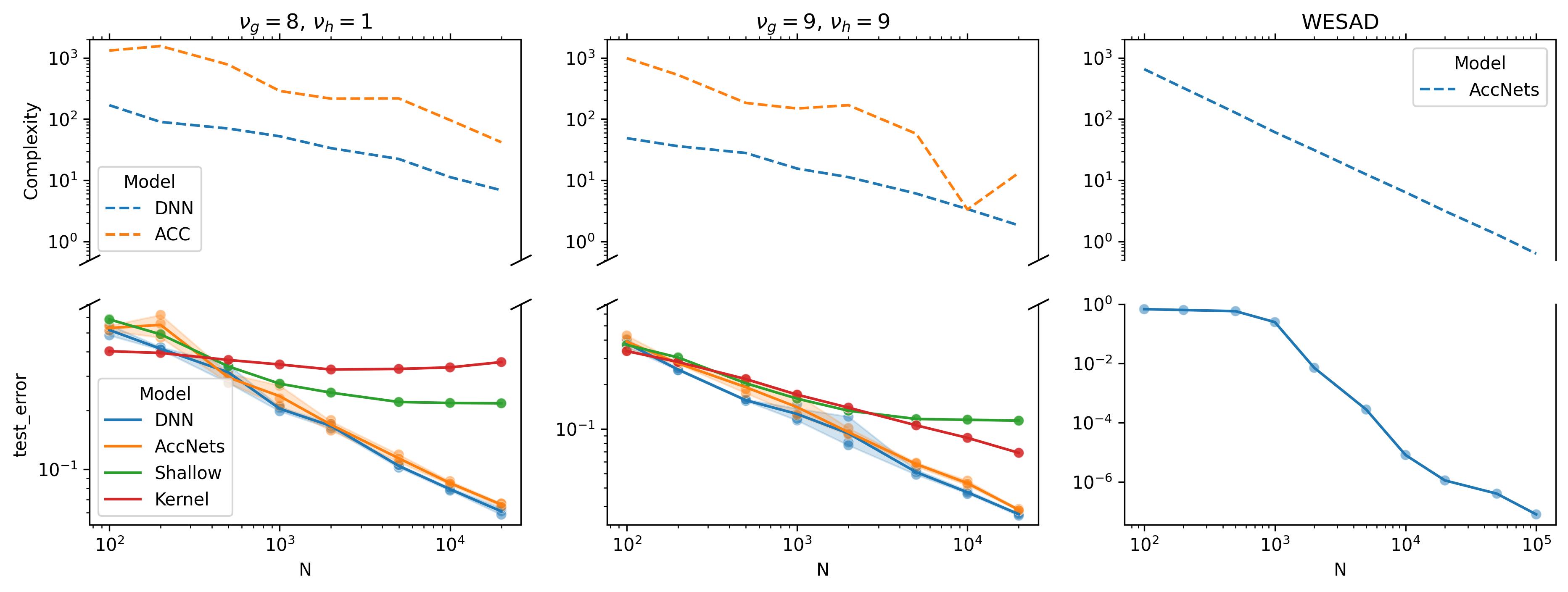
Figure 1: Visualization of scaling laws. We observe that deep networks (either AccNets or DNNs) achieve better scaling laws than kernel methods or shallow networks on certain compositional tasks, in agreement with our theory. We also see that our new generalization bounds approximately recover the right saling laws (even though they are orders of magnitude too large overall). We consider a compositional true function $f^{*}=h\circ g$ where $g$ maps from dimension 15 to 3 while h maps from 3 to 20, and we denote $\nu_{g},\nu_{h}$ for the number of times $g,h$ are differentiable. In the first plot $\nu_{g}=8,\nu_{h}=1$ so that $g$ is easy to learn while $h$ is hard, whereas in the second plot $\nu_{g}=9,\nu_{h}=9$, so both $g$ and $h$ are relatively easier. The third plot presents the decay in test error and generalization bounds for networks evaluated using the real-world dataset, WESAD [38].

4 Breaking the Curse of Dimensionality with Compositionality

In this section we study a large family of functions spaces, obtained by taking compositions of Sobolev balls. We focus on this family of tasks because they are well adapted to the complexity measure we have identified, and because kernel methods and even shallow networks do suffer from the curse of dimensionality on such tasks, whereas deep networks avoid it (e.g. Figure 1).

More precisely, we will show that these sets of functions can be approximated by a AccNets with bounded (or in some cases slowly growing) complexity measure

$$R(\theta)=\prod_{\ell=1}^{L}Lip(f_{\ell})\sum_{\ell=1}^{L}\frac{\left\|f_{\ell}\right\|_{F_{1}}}{Lip(f_{\ell})}\sqrt{d_{\ell}+d_{\ell-1}}.$$

This will then allow us show that AccNets can (assuming global convergence) avoid the curse of dimensionality, even in settings that should suffer from the curse of dimensionality, when the input dimension is large and the function is not very smooth (only a few times differentiable).

Since the regularization term $R(\theta)$ is difficult to optimize directly because of the Lipschitz constants, we also consider the upper bound $\tilde{R}(\theta)$ obtained by replacing each $Lip(f_{\ell})$ with $\|V_{\ell}\|_{op}\|W_{\ell}\|_{op}$.

4.1 Composition of Sobolev Balls

The family of Sobolev norms capture some notion of regularity of a function, as it measures the size of its derivatives. The Sobolev norm of a function $f:\mathbb{R}^{d_{in}}\to\mathbb{R}$ is defined in terms of its derivatives $\partial_{x}^{\alpha}f$ for some $d_{in}$-multi-index $\alpha$, namely the $W^{\nu,p}(\pi)$-Sobolev norm with integer $\nu$ and $p\geq 1$ is defined as

$$\left\|f\right\|^{p}_{W^{\nu,p}(\pi)}=\sum_{\left|\alpha\right|\leq\nu}\left\|\partial_{x}^{\alpha}f\right\|_{L_{p}(\pi)}^{p}.$$

Note that the derivative $\partial_{x}^{\alpha}f$ only needs to be defined in the ‘weak’ sense, which means that even non-differentiable functions such as the ReLU functions can actually have finite Sobolev norm.

The Sobolev balls $B_{W^{\nu,p}(\pi)}(0,R)=\{f:\left\|f\right\|_{W^{\nu,p}(\pi)}\leq R\}$ are a family of function spaces with a range of regularity (the larger $\nu$, the more regular). This regularity makes these spaces of functions learnable purely from the fact that they enforce the function $f$ to vary slowly as the input changes. Indeed we can prove the following generalization bound:

Proposition 3.

Given a distribution $\pi$ with support the $L_{2}$ ball with radius b, we have that with probability $1-\delta$ for all functions $f\in\mathcal{F}=\left\{f:\left\|f\right\|_{W^{\nu,2}}\leq R,\left\|f\right\|_{\infty}\leq R\right\}$

$$\mathcal{L}(f)-\tilde{\mathcal{L}}_{N}(f)\leq 2\rho C_{1}RE_{\nicefrac{{\nu}}{{d}}}(N)+c_{0}\sqrt{\frac{2\log\nicefrac{{2}}{{\delta}}}{N}}.$$

where $E_{r}(N)=N^{-\frac{1}{2}}$ if $r>\frac{1}{2}$, $E_{r}(N)=N^{-\frac{1}{2}}\log N$ if $r=\frac{1}{2}$, and $E_{r}(N)=N^{-r}$ if $r<\frac{1}{2}$.

But this result also illustrates the curse of dimensionality: the differentiability $\nu$ needs to scale with the input dimension $d_{in}$ to obtain a reasonable rate. If instead $\nu$ is constant and $d_{in}$ grows, then the number of datapoints $N$ needed to guarantee a generalization gap of at most $\epsilon$ scales exponentially in $d_{in}$, i.e. $N\sim\epsilon^{-\frac{d_{in}}{\nu}}$. One way to interpret this issue is that regularity becomes less and less useful the larger the dimension: knowing that similar inputs have similar outputs is useless in high dimension where the closest training point $x_{i}$ to a test point $x$ is typically very far away.

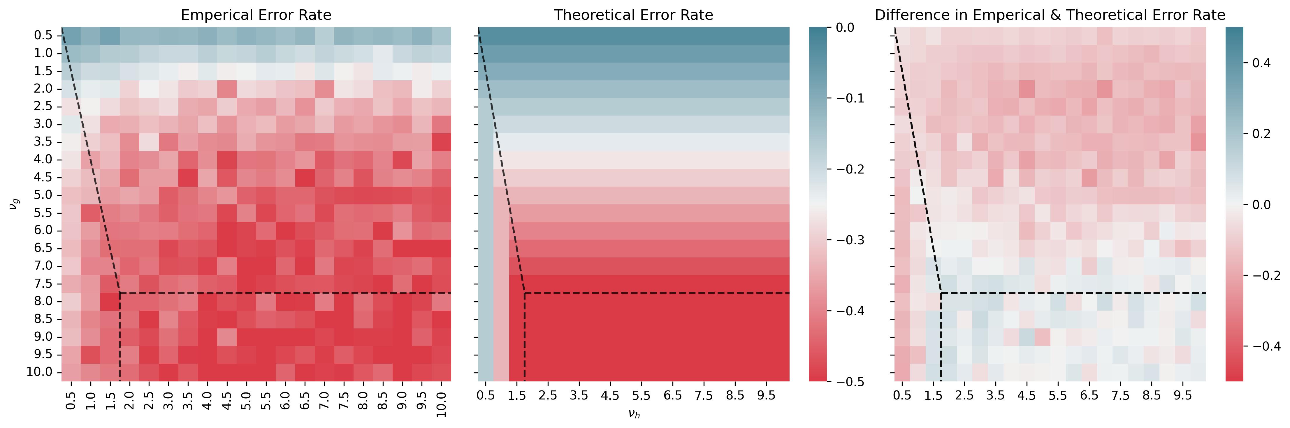
Figure 2: A comparison of empirical and theoretical error rates. The first plot illustrates the log decay rate of the test error with respect to the dataset size $N$ based on our empirical simulations. The second plot depicts the theoretical decay rate of the test error as discussed in Section 4.1, $-\min\{\frac{1}{2},\frac{\nu_{g}}{d_{in}},\frac{\nu_{h}}{d_{mid}}\}$. The final plot on the right displays the difference between the two. The lower left region represents the area where $g$ is easier to learn than $h$, the upper right where $h$ is easier to learn than $g$, and the lower right region where both $f$ and $g$ are easy.

.

4.1.1 Breaking the Curse of Dimensionality with Compositionality

To break the curse of dimensionality, we need to assume some additional structure on the data or task which introduces an ‘intrinsic dimension’ that can be much lower than the input dimension $d_{in}$:

Manifold hypothesis: If the input distribution lies on a $d_{surf}$-dimensional manifold, the error rates typically depends on $d_{surf}$ instead of $d_{in}$ [39, 10].

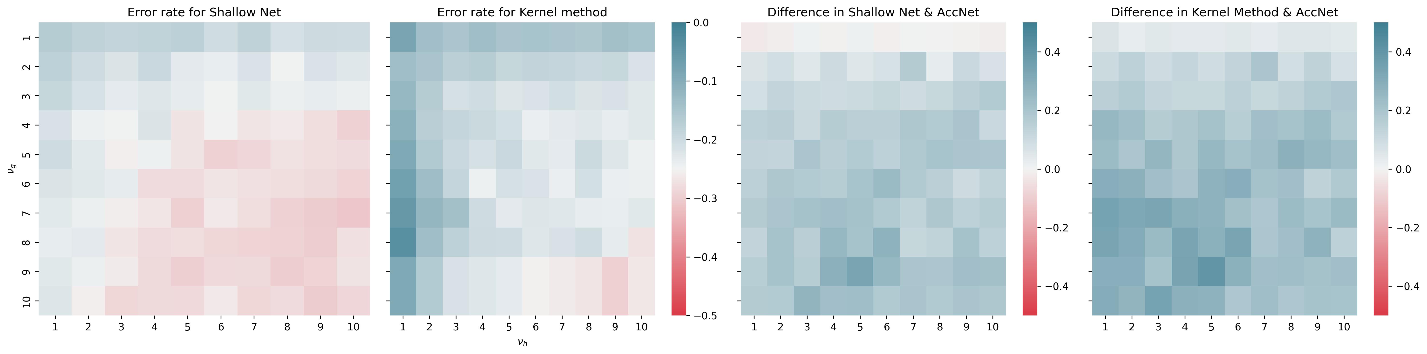
Figure 3: Comparing error rates for shallow and AccNets: shallow nets vs. AccNets, and kernel methods vs. AccNets. The left two graphs shows the empirical decay rate of test error with respect to dataset size (N) for both shallow nets and kernel methods. In contrast to our earlier empirical findings for AccNets, both shallow nets and kernel methods exhibit a slower decay rate in test error. The right two graphs present the differences in log decay rates between shallow nets and AccNets, as well as between kernel methods and AccNets. AccNets almost always obtain better rates, with a particularly large advantage at the bottom and middle-left.

.

Known Symmetries: If $f^{*}(g\cdot x)=f^{*}(x)$ for a group action $\cdot$ w.r.t. a group $G$, then $f^{*}$ can be written as the composition of a modulo map $g^{*}:\mathbb{R}^{d_{in}}\to\nicefrac{{\mathbb{R}^{d_{in}}}}{{G}}$ which maps pairs of inputs which are equivalent up to symmetries to the same value (pairs $x,y$ s.t. $y=g\cdot x$ for some $g\in G$), and then a second function $h^{*}:\nicefrac{{\mathbb{R}^{d_{in}}}}{{G}}\to\mathbb{R}^{d_{out}}$, then the complexity of the task will depend on the dimension of the modulo space $\nicefrac{{\mathbb{R}^{d_{in}}}}{{G}}$ which can be much lower. If the symmetry is known, then one can for example fix $g^{*}$ and only learn $h^{*}$ (though other techniques exist, such as designing kernels or features that respect the same symmetries) [31].

Symmetry Learning: However if the symmetry is not known then both $g^{*}$ and $h^{*}$ have to be learned, and this is where we require feature learning and/or compositionality. Shallow networks are able to learn translation symmetries, since they can learn so-called low-index functions which satisfy $f^{*}(x)=f^{*}(Px)$ for some projection $P$ (with a statistical complexity that depends on the dimension of the space one projects into, not the full dimension [5, 2]). Low-index functions correspond exactly to the set of functions that are invariant under translation along the kernel $\ker P$. To learn general symmetries, one needs to learn both $h^{*}$ and the modulo map $g^{*}$ simultaneously, hence the importance of feature learning.

For $g^{*}$ to be learnable efficiently, it needs to be regular enough to not suffer from the curse of dimensionality, but many traditional symmetries actually have smooth modulo maps, for example the modulo map $g^{*}(x)=\left\|x\right\|^{2}$ for rotation invariance. This can be understood as a special case of composition of Sobolev functions, whose generalization gap can be bounded:

Theorem 4.

Consider the function set $\mathcal{F}=\mathcal{F}_{L}\circ\cdots\circ\mathcal{F}_{1}$ where $\mathcal{F}_{\ell}=\left\{f_{\ell}:\mathbb{R}^{d_{\ell-1}}\to\mathbb{R}^{d_{\ell}}\text{ s.t. }\left\|f_{\ell}\right\|_{W^{\nu_{\ell},2}}\leq R_{\ell},\left\|f_{\ell}\right\|_{\infty}\leq b_{\ell},Lip(f_{\ell})\leq\rho_{\ell}\right\}$, and let $r_{min}=\min_{\ell}r_{\ell}$ for $r_{\ell}=\frac{\nu_{\ell}}{d_{\ell-1}}$, then with probability $1-\delta$ we have for all $f\in\mathcal{F}$

$$\mathcal{L}(f)-\tilde{\mathcal{L}}_{N}(f) \leq\rho C_{0}\left(\sum_{\ell=1}^{L}\left(C_{\ell}\rho_{L:\ell+1}R_{\ell}\right)^{\frac{1}{r_{min}+1}}\right)^{r_{min}+1}E_{r_{min}}(N)+c_{0}\sqrt{\frac{2\log\nicefrac{{2}}{{\delta}}}{N}},$$

where $C_{\ell}$ depends only on $d_{\ell-1},d_{\ell},\nu_{\ell},b_{\ell-1}$.

We see that only the smallest ratio $r_{min}$ matters when it comes to the rate of learning. And actually the above result could be slightly improved to show that the sum over all layers could be replaced by a sum over only the layers where the ratio $r_{\ell}$ leads to the worst rate $E_{r_{\ell}}(N)=E_{r_{min}}(N)$ (and the other layers contribute an asymptotically subdominant amount).

Coming back to the symmetry learning example, we see that the hardness of learning a function of the type $f^{*}=h\circ g$ with inner dimension $d_{mid}$ and regularities $\nu_{g}$ and $\nu_{h}$, the error rate will be (up to log terms) $N^{-\min\{\frac{1}{2},\frac{\nu_{g}}{d_{in}},\frac{\nu_{h}}{d_{mid}}\}}$. This suggests the existence of three regimes depending on which term attains the minimum: a regime where both $g$ and $h$ are easy to learn and we have $N^{-\frac{1}{2}}$ learning, a regime $g$ is hard, and a regime where $h$ is hard. The last two regimes differentiate between tasks where learning the symmetry is hard and those where learning the function knowing its symmetries is hard.

In contrast, without taking advantage of the compositional structure, we expect $f^{*}$ to be only $\min\{\nu_{g},\nu_{h}\}$ times differentiable, so trying to learn it as a single Sobolev function would lead to an error rate of $N^{-\min\{\frac{1}{2},\frac{\min\{\nu_{g},\nu_{h}\}}{d_{in}}\}}=N^{-\min\{\frac{1}{2},\frac{\nu_{g}}{d_{in}},\frac{\nu_{h}}{d_{in}}\}}$ which is no better than the compositional rate, and is strictly worse whenever $\nu_{h}<\nu_{g}$ and $\frac{\nu_{h}}{d_{in}}<\frac{1}{2}$ (we can always assume $d_{mid}\leq d_{in}$ since one could always choose $d=id$).

Furthermore, since multiple compositions are possible, one can imagine a hierarchy of symmetries that slowly reduce the dimensionality with less and less regular modulo maps. For example one could imagine a composition $f_{L}\circ\cdots\circ f_{1}$ with dimensions $d_{\ell}=d_{0}2^{-\ell}$ and regularities $\nu_{\ell}=d_{0}2^{-\ell}$ so that the ratios remain constant $r_{\ell}=\frac{d_{0}2^{-\ell}}{d_{0}2^{-\ell+1}}=\frac{1}{2}$, leading to an almost parametric rate of $N^{-\frac{1}{2}}\log N$ even though the function may only be $d_{0}2^{-L}$ times differentiable. Without compositionality, the rate would only be $N^{-2^{-L}}$.

Remark.

In the case of a single Sobolev function, one can show that the rate $E_{\nicefrac{{\nu}}{{d}}}(N)$ is in some sense optimal, by giving an information theoretic lower bound with matching rate. A naive argument suggests that the rate of $E_{\min\{r_{1},\dots,r_{L}\}}(N)$ should similarly be optimal: assume that the minimum $r_{\ell}$ is attained at a layer $\ell$, then one can consider the subset of functions such that the image $f_{\ell-1:1}(B(0,r))$ contains a ball $B(z,r^{\prime})\subset\mathbb{R}^{d_{\ell-1}}$ and that the function $f_{L:\ell+1}$ is $\beta$-non-contracting $\left\|f_{L:\ell+1}(x)-f_{L:\ell+1}(y)\right\|\geq\beta\left\|x-y\right\|$, then learning $f_{L:1}$ should be as hard as learning $f_{\ell}$ over the ball $B(z,r^{\prime})$ (more rigorously this could be argued from the fact that any $\epsilon$-covering of $f_{L:1}$ can be mapped to an $\nicefrac{{\epsilon}}{{\beta}}$-covering of $f_{\ell}$), thus forcing a rate of at least $E_{r_{\ell}}(N)=E_{\min\{r_{1},\dots,r_{L}\}}(N)$.

An analysis of minimax rates in a similar setting has been done in [22].

Remark.

The type of model that seems most appropriate to learning composition of Sobolev functions are arguably Deep Gaussian Processes (DGP). While it should be relatively straightforward to use DGP with a Lipschitzness constraint to recover optimal rates when the dimensions $d_{\ell}$ and differentiabilities $\nu_{\ell}$ of the true functions are known in advance, it might not possible in general. We will show that AccNet can recover almost optimal rates thanks to the adaptivity of the $F_{1}$ norm.

4.2 Breaking the Curse of Dimensionality with AccNets

Now that we know that composition of Sobolev functions can be easily learnable, even in settings where the curse of dimensionality should make it hard to learn them, we need to find a model that can achieve those rates. Though many models are possible , we focus on DNNs, in particular AccNets. Assuming convergence to a global minimum of the loss of sufficiently wide AccNets with two types of regularization, one can guarantee close to optimal rates:

Theorem 5.

Given a true function $f_{L^{*}:1}^{*}=f_{L^{*}}^{*}\circ\cdots\circ f_{1}^{*}$ going through the dimensions $d_{0}^{*},\dots,d_{L^{*}}^{*}$, along with a continuous input distribution $\pi_{0}$ supported in $B(0,b_{0})$, such that the distributions $\pi_{\ell}$ of $f_{\ell}^{*}(x)$ (for $x\sim\pi_{0}$) are continuous too and supported inside $B(0,b_{\ell})\subset\mathbb{R}^{d_{\ell}^{*}}$. Further assume that there are differentiabilities $\nu_{\ell}$ and radii $R_{\ell}$ such that $\left\|f_{\ell}^{*}\right\|_{W^{\nu_{\ell},2}(B(0,b_{\ell}))}\leq R_{\ell}$, and $\rho_{\ell}$ such that $Lip(f_{\ell}^{*})\leq\rho_{\ell}$. For an infinite width AccNet with $L\geq L^{*}$ and dimensions $d_{\ell}\geq d_{1}^{*},\dots,d_{L^{*}-1}^{*}$, we have for the ratios $\tilde{r}_{\ell}=\frac{\nu_{\ell}}{d_{\ell}^{*}+3}$:

(1) At a global min $\hat{f}_{L:1}$ of $\tilde{\mathcal{L}}_{N}(f_{L:1})+\lambda R(\theta)$, we have $\mathcal{L}(\hat{f}_{L:1})=\tilde{O}(N^{-\min\{\frac{1}{2},\tilde{r}_{1},\dots,\tilde{r}_{L^{*}}\}})$.

(2) At a global min $\hat{f}_{L:1}$ of $\tilde{\mathcal{L}}_{N}(f_{L:1})+\lambda\tilde{R}(\theta)$, we have $\mathcal{L}(\hat{f}_{L:1})=\tilde{O}(N^{-\frac{1}{2}+\sum_{\ell=1}^{L^{*}}\max\{0,\tilde{r}_{\ell}-\frac{1}{2}\}})$.

There are a number of limitations to this result. First we assume that one is able to recover the global minimizer of the regularized loss, which should be hard in general (we already know from [5] that this is NP-hard for shallow networks and a simple $F_{1}$-regularization). Note that it is sufficient to recover a network $f_{L:1}$ whose regularized loss is within a constant of the global minimum, which might be easier to guarantee, but should still be hard in general. The typical method of training with GD on the regularized loss is a greedy approach, which might fail in general but could recover almost optimal parameters under the right conditions (some results suggest that training relies on first order correlations to guide the network in the right direction [2, 1, 36]).

We propose two regularizations because they offer a tradeoff:

First regularization: The first regularization term leads to almost optimal rates, up to the change from $r_{\ell}=\frac{\nu_{\ell}}{d_{\ell}^{*}}$ to $r_{\ell}=\frac{\nu_{\ell}}{d_{\ell}^{*}+3}$ which is negligible for large dimensions $d_{\ell}$ and differentiabilities $\nu_{\ell}$. The first problem is that it requires an infinite width at the moment, because we were not able to prove that a function with bounded $F_{1}$-norm and Lipschitz constant can be approximated by a sufficiently wide shallow networks with the same (or close) $F_{1}$-norm and Lipschitz constant (we know from [5] that it is possible without preserving the Lipschitzness). We are quite hopeful that this condition might be removed in future work.

The second and more significant problem is that the Lipschitz constants $Lip(f_{\ell})$ are difficult to optimize over. For finite width networks it is in theory possible to take the max over all linear regions, but the complexity might be unreasonable. It might be more reasonable to leverage an implicit bias instead, such as a large learning rate, because a large Lipschitz constant implies that the nework is sensible to small changes in its parameters, so GD with a large learning rate should only converge to minima with a small Lipschitz constant (such a bias is described in [26]). It might also be possible to replace the Lipschitz constant in our generalization bounds, possibly along the lines of [45].

Second regularization: The second regularization term has the advantage that it can be optimized with GD. Furthermore it does not require an infinite width, only a sufficiently large one. The issue is that it leads to rates that could be far from optimal depending on the ratios $\tilde{r}_{\ell}$: it recovers the same rate as the first regularization term if no more than one ratio $\tilde{r}_{\ell}$ is smaller than $\frac{1}{2}$, but if many of these ratios are above $\frac{1}{2}$, it can be arbitrarily smaller.

In Figure 2, we compare the empirical rates (by doing a linear fit on a log-log plot of test error as a function of $N$) and the predicted optimal rates $\min\{\frac{1}{2},\frac{\nu_{g}}{d_{in}},\frac{\nu_{h}}{d_{mid}}\}$ and observe a pretty good match.

Remark.

As can be seen in the proof of Theorem5, when the depth $L$ is strictly larger than the true depth $L^{*}$, one needs to add identity layers, leading to a so-called Bottleneck structure, which was proven emerge as a result of weight decay in [27, 26, 47]. These identity layers add a term that scales linearly in the additional depth $\frac{(L-L^{*})d_{min}^{*}}{\sqrt{N}}$ to the first regularization, and an exponential prefactor $(2d_{min}^{*})^{L-L^{*}}$ to the second.

5 Conclusion

We have given a generalization bound for Accordion Networks and as an extension Fully-Connected networks. It depends on $F_{1}$-norms and Lipschitz constants of its shallow subnetworks. This allows us to prove under certain assumptions that AccNets can learn general compositions of Sobolev functions efficiently, making them able to break the curse of dimensionality in certain settings, such as in the presence of unknown symmetries.

The Appendix is structured as follows:

1. In Section A, we describe the experimental setup and provide a few additional experiments.

2. In Section B, we prove Theorems 1 and 2 from the main.

3. In Section C, we prove Proposition 3 and Theorem 4.

4. In Section D, we prove Theorem 5 and other approximation results concerning Sobolev functions.

5. In Section E, we prove a few technical results on the covering number.

Appendix A Experimental Setup

In this section, we review our numerical experiments and their setup both on synthetic and real-world datasets in order to address theoretical results more clearly and intuitively.

The code used for experiments is publicly available here.

A.1 Dataset

A.1.1 Emperical Dataset

The Matérn kernel is considered a generalization of the radial basis function (RBF) kernel. It controls the differentiability, or smoothness, of the kernel through the parameter $\nu$. As $\nu\rightarrow\infty$, the Matérn kernel converges to the RBF kernel, and as $\nu\rightarrow 0$, it converges to the Laplacian kernel, a 0-differentiable kernel. In this study, we utilized the Matérn kernel to generate Gaussian Process (GP) samples based on the composition of two Matérn kernels, $K_{g}$ and $K_{h}$, with varying differentiability in the range [0.5,10]×[0.5,10]. The input dimension ($d_{in}$) of the kernel, the bottleneck mid-dimension ($d_{mid}$), and the output dimension ($d_{out}$) are 15, 3, and 20, respectively.

This outlines the general procedure of our sampling method for synthetic data:

1. Sample the training dataset $X\in\mathbb{R}^{D\times d_{in}}$

2. From X, compute the $D\times D$ kernel $K_{g}$ with given $\nu_{g}$

3. From $K_{g}$, sample $Z\in\mathbb{R}^{D\times d_{mid}}$ with columns sampled from the Gaussian $\mathcal{N}(0,K_{g})$.

4. From $Z$, compute $K_{g}$ with given $\nu_{h}$

5. From $K_{h}$, sample the test dataset $Y\in\mathbb{R}^{D\times d_{out}}$ with columns sampled from the Gaussian $\mathcal{N}(0,K_{h})$.

We utilized four AMD Opteron 6136 processors (2.4 GHz, 32 cores) and 128 GB of RAM to generate our synthetic dataset. The maximum possible dataset size for 128 GB of RAM is approximately 52,500; however, we opted for a synthetic dataset size of 22,000 due to the computational expense associated with sampling the Matérn kernel. This decision was made considering the time complexity of $\mathcal{O}(n^{3})$and the space complexity of $\mathcal{O}(n^{2})$ involved. Out of the 22,000 dataset points, 20,000 were allocated for training data, and 2,000 were used for the test dataset

A.1.2 Real-world dataset: WESAD

In our study, we utilized the Wearable Stress and Affect Detection (WESAD) dataset to train our AccNets for binary classification. The WESAD dataset, which is publicly accessible, provides multimodal physiological and motion data collected from 15 subjects using devices worn on the wrist and chest. For the purpose of our experiment, we specifically employed the Empatica E4 wrist device to distinguish between non-stress (baseline) and stress conditions, simplifying the classification task to these two categories.

After preprocessing, the dataset comprised a total of 136,482 instances. We implemented a train-test split ratio of approximately 75:25, resulting in 100,000 instances for the training set and 36,482 instances for the test set. The overall hyperparameters and architecture of the AccNets model applied to the WESAD dataset were largely consistent with those used for our synthetic data. The primary differences were the use of 100 epochs for each iteration of Ni from Ns, and a learning rate set to 1e-5.

A.2 Model setups

To investigate the scaling law of test error for our synthetic data, we trained models using $N_{i}$ datapoints from our training data, where $N=[100,200,500,1000,2000,5000,10000,20000]$. The models employed for this analysis included the kernel method, shallow networks, fully connected deep neural networks (FC DNN), and AccNets. For FC DNN and AccNets, we configured the network depth to 12 layers, with the layer widths set as $[d_{in},500,500,...,500,d_{out}]$ for DNNs, and $[d_{i}n,900,100,900,...,100,900,d_{out}]$ for AccNets.

To ensure a comparable number of neurons, the width for the shallow networks was set to 50,000, resulting in dimensions of $[d_{in},50000,d_{out}]$.

We utilized ReLU as the activation function and $L^{1}$-norm as the cost function, with the Adam optimizer. The total number of batch was set to 5, and the training process was conducted over 3600 epochs, divided into three phases. The detailed optimizer parameters are as follows:

1. For the first 1200 epochs: learning rate $(lr)=1.5*0.001$, weight decay = 0

2. For the second 1200 epochs: $lr=0.4*0.001$, weight decay $=0.002$

3. For the final 1200 epochs: $lr=0.1*0.001$, weight decay $=0.005$

We conducted experiments utilizing 12 NVIDIA V100 GPUs (each with 32GB of memory) over a period of 6.3 days to train the synthetic dataset. In contrast, training the WESAD dataset required only one hour on a single V100 GPU.

Figure 4: A comparison: singular values of the weight matrices for DNN and AccNets models. The first two plots represent cases where $N$ = 10000 while the right two plots correspond to $N$ = 200.The number of outliers at the top of each plot signifies the rank of each network. The plots with $N=10000$ datasets demonstrate a clearer capture of the true rank compared to those with $N=200$ indicating that a higher dataset count provides more accurate rank determination.

Appendix B AccNet Generalization Bounds

The proof of generalization for shallow networks (Theorem 1) is the special case $L=1$ of the proof of Theorem 2, so we only prove the second:

Theorem 6.

Consider an accordion net of depth $L$ and widths $d_{L},\dots,d_{0}$, with corresponding set of functions $\mathcal{F}=\{f_{L:1}:\left\|f_{\ell}\right\|_{F_{1}}\leq R_{\ell},\text{Lip}(f_{\ell})\leq\rho_{\ell}\}$ with input space $\Omega=B(0,r)$. For any $\rho$-Lipschitz loss function $\ell(x,f(x))$ with $\left|\ell(x,y)\right|\leq c_{0}$, we know that with probability $1-\delta$ over the sampling of the training set $X$ from the distribution $\pi$, we have for all $f\in\mathcal{F}$

$$\mathcal{L}(f)-\tilde{\mathcal{L}}_{N}(f) \leq C\rho_{L:1}r\sum_{\ell^{\prime}=1}^{L}\frac{R_{\ell^{\prime}}}{\rho_{\ell^{\prime}}}\sqrt{d_{\ell^{\prime}}+d_{\ell^{\prime}-1}}\frac{\log N}{\sqrt{N}}(1+o(1))+c_{0}\sqrt{\frac{2\log\nicefrac{{2}}{{\delta}}}{N}}.$$

Proof.

The strategy is: (1) prove a covering number bound on $\mathcal{F}$ (2) use it to obtain a Rademacher complexity bound, (3) use the Rademacher complexity to bound the generalization error.

(1) We define $f_{\ell}=V_{\ell}\circ\sigma\circ W_{\ell}$ so that $f_{\theta}=f_{L:1}=f_{L}\circ\cdots\circ f_{1}$. First notice that we can write each $f_{\ell}$ as convex combination of its neurons:

$$f_{\ell}(x)=\sum_{i=1}^{w_{\ell}}v_{\ell,i}\sigma(w_{\ell,i}^{T}x)=R_{\ell}\sum_{i=1}^{w_{\ell}}c_{\ell,i}\bar{v}_{\ell,i}\sigma(\bar{w}_{\ell,i}^{T}x)$$

for $\bar{w}_{\ell,i}=\frac{w_{\ell,i}}{\left\|w_{\ell,i}\right\|}$, $\bar{v}_{\ell,i}=\frac{v_{\ell,i}}{\left\|v_{\ell,i}\right\|}$, $R_{\ell}=\sum_{i=1}^{\ell}\left\|v_{\ell,i}\right\|\left\|w_{\ell,i}\right\|$ and $c_{\ell,i}=\frac{1}{R_{\ell}}\left\|v_{\ell,i}\right\|\left\|w_{\ell,i}\right\|$.

Let us now consider a sequence $\epsilon_{k}=2^{-k}$ for $k=0,\dots,K$ and define $\tilde{v}_{\ell,i}^{(k)},\tilde{w}_{\ell,i}^{(k)}$ to be the $\epsilon_{k}$-covers of $\bar{v}_{\ell,i},\bar{w}_{\ell,i}$, furthermore we may choose $\tilde{v}_{\ell,i}^{(0)}=\tilde{w}_{\ell,i}^{(0)}=0$ since every unit vector is within a $\epsilon_{0}=1$ distance of the origin. We will now show that on can approximate $f_{\theta}$ by approximating each of the $f_{\ell}$ by functions of the form

$$\tilde{f}_{\ell}(x)=R_{\ell}\sum_{k=1}^{K_{\ell}}\frac{1}{M_{k,\ell}}\sum_{m=1}^{M_{k,\ell}}\tilde{v}_{\ell,i_{\ell,m}^{(k)}}^{(k)}\sigma(\tilde{w}_{\ell,i_{\ell,m}^{(k)}}^{(k)T}x)-\tilde{v}_{\ell,i_{\ell,m}^{(k)}}^{(k-1)}\sigma(\tilde{w}_{\ell,i_{\ell,m}^{(k)}}^{(k-1)T}x)$$

for indices $i_{\ell,m}^{(k)}=1,\dots,w_{\ell}$ choosen adequately. Notice that the number of functions of this type equals the number of $M_{k,\ell}$ quadruples $(\tilde{v}_{\ell,i_{\ell,m}^{(k)}}^{(k)},\tilde{w}_{\ell,i_{\ell,m}^{(k)}}^{(k)T},\tilde{v}_{\ell,i_{\ell,m}^{(k)}}^{(k-1)},\tilde{w}_{\ell,i_{\ell,m}^{(k)}}^{(k-1)T})$ where these vectors belong to the $\epsilon_{k}$- resp. $\epsilon_{k-1}$-coverings of the $d_{in}$- resp. $d_{out}$-dimensional unit sphere. Thus the number of such functions is bounded by

$$\prod_{k=1}^{K_{\ell}}\left(\mathcal{N}_{2}(\mathbb{S}^{d_{in}-1},\epsilon_{k})\mathcal{N}_{2}(\mathbb{S}^{d_{out}-1},\epsilon_{k})\mathcal{N}_{2}(\mathbb{S}^{d_{in}-1},\epsilon_{k-1})\mathcal{N}_{2}(\mathbb{S}^{d_{out}-1},\epsilon_{k-1})\right)^{M_{k,\ell}},$$

and we have this choice for all $\ell=1,\dots,L$. We will show that with sufficiently large $M_{k,\ell}$ this set of functions $\epsilon$-covers $\mathcal{F}$ which then implies that

$$\log\mathcal{N}_{2}(\mathcal{F},\epsilon)\leq 2\sum_{\ell=1}^{L}\sum_{k=1}^{K_{\ell}}M_{k,\ell}\left(\log\mathcal{N}_{2}(\mathbb{S}^{d_{in}-1},\epsilon_{k-1})+\log\mathcal{N}_{2}(\mathbb{S}^{d_{in}-1},\epsilon_{k-1})\right).$$

We will use the probabilistic method to find the right indices $i_{\ell,m}^{(k)}$ to approximate a function $f_{\ell}=R_{\ell}\sum_{i=1}^{w_{\ell}}c_{\ell,i}\bar{v}_{\ell,i}\sigma(\bar{w}_{\ell,i}^{T}x)$ with a function $\tilde{f}_{\ell}$. We take all $i_{\ell,m}^{(k)}$ to be i.i.d. equal to the index $i=1,\cdots,w_{\ell}$ with probability $c_{\ell,i}$, so that in expectation

$$\mathbb{E}\tilde{f}_{\ell}(x) =R_{\ell}\sum_{k=1}^{K_{\ell}}\sum_{i=1}^{w_{\ell}}c_{\ell,i}\left(\tilde{v}_{\ell,i}^{(k)}\sigma(\tilde{w}_{\ell,i}^{(k)T}x)-\tilde{v}_{\ell,i}^{(k-1)}\sigma(\tilde{w}_{\ell,i}^{(k-1)T}x)\right)$$

$$=R_{\ell}\sum_{i=1}^{w_{\ell}}c_{\ell,i}\tilde{v}_{\ell,i}^{(K)}\sigma(\tilde{w}_{\ell,i}^{(K)T}x).$$

We will show that this expectation is $O(\epsilon_{K_{\ell}})$-close to $f_{\ell}$ and that the variance of $\tilde{f}_{\ell}$ goes to zero as the $M_{\ell,k}$s grow, allowing us to bound the expected error $\mathbb{E}\left\|f_{L:1}-\tilde{f}_{L:1}\right\|_{\pi}^{2}\leq\text{$\epsilon$}^{2}$ which then implies that there must be at least one choice of indices $i_{\ell,m}^{(k)}$ such that $\left\|f_{L:1}-\tilde{f}_{L:1}\right\|_{\pi}\leq\epsilon$.

Let us first bound the distance

$$\left\|f_{\ell}(x)-\mathbb{E}\tilde{f}_{\ell}(x)\right\| =R_{\ell}\left\|\sum_{i=1}^{w_{\ell}}c_{\ell,i}\left(\bar{v}_{\ell,i}\sigma(\bar{w}_{\ell,i}^{T}x)-\tilde{v}_{\ell,i}^{(K)}\sigma(\tilde{w}_{\ell,i}^{(K)T}x)\right)\right\|$$

$$\leq R_{\ell}\sum_{i=1}^{w_{\ell}}c_{\ell,i}\left(\left\|\left(\bar{v}_{\ell,i}-\tilde{v}_{\ell,i}^{(K)}\right)\sigma(\bar{w}_{\ell,i}^{T}x)\right\|+\left\|\tilde{v}_{\ell,i}^{(K)}\left(\sigma(\bar{w}_{\ell,i}^{T}x)-\sigma(\tilde{w}_{\ell,i}^{(K)T}x)\right)\right\|\right)$$

$$\leq R_{\ell}\sum_{i=1}^{w_{\ell}}c_{\ell,i}\left(\left\|\bar{v}_{\ell,i}-\tilde{v}_{\ell,i}^{(K)}\right\|\left\|\bar{w}_{\ell,i}^{T}x\right\|+\left\|\tilde{v}_{\ell,i}^{(K)}\right\|\left\|\bar{w}_{\ell,i}^{T}x-\tilde{w}_{\ell,i}^{(K)T}x\right\|\right)$$

$$\leq 2R_{\ell}\sum_{i=1}^{w_{\ell}}c_{\ell,i}\epsilon_{K_{\ell}}\left\|x\right\|$$

$$=2R_{\ell}\epsilon_{K_{\ell}}\left\|x\right\|.$$

Then we bound the trace of the covariance of $\tilde{f}_{\ell}$ which equals the expected square distance between $\tilde{f}_{\ell}$ and its expectation:

$$\mathbb{E}\left\|\tilde{f}_{\ell}(x)-\mathbb{E}\tilde{f}_{\ell}(x)\right\|^{2}$$

$$=\sum_{k=1}^{K_{\ell}}\frac{R_{\ell}^{2}}{M_{k,\ell}^{2}}\sum_{m=1}^{M_{k,\ell}}\mathbb{E}\left\|\tilde{v}_{\ell,i_{\ell,m}^{(k)}}^{(k)}\sigma(\tilde{w}_{\ell,i_{\ell,m}^{(k)}}^{(k)T}x)-\tilde{v}_{\ell,i_{\ell,m}^{(k)}}^{(k-1)}\sigma(\tilde{w}_{\ell,i_{\ell,m}^{(k)}}^{(k-1)T}x)-\mathbb{E}\left[\tilde{v}_{\ell,i_{\ell,m}^{(k)}}^{(k)}\sigma(\tilde{w}_{\ell,i_{\ell,m}^{(k)}}^{(k)T}x)-\tilde{v}_{\ell,i_{\ell,m}^{(k)}}^{(k-1)}\sigma(\tilde{w}_{\ell,i_{\ell,m}^{(k)}}^{(k-1)T}x)\right]\right\|^{2}$$

$$\leq\sum_{k=1}^{K_{\ell}}\frac{R_{\ell}^{2}}{M_{k,\ell}^{2}}\sum_{m=1}^{M_{k,\ell}}\mathbb{E}\left\|\tilde{v}_{\ell,m}^{(k)}\sigma(\tilde{w}_{\ell,m}^{(k)T}x)-\tilde{v}_{\ell,m}^{(k-1)}\sigma(\tilde{w}_{\ell,m}^{(k-1)T}x)\right\|^{2}$$

$$=\sum_{k=1}^{K_{\ell}}\frac{R_{\ell}^{2}}{M_{k,\ell}}\sum_{i=1}^{w_{\ell}}c_{i}\left\|\tilde{v}_{\ell,i}^{(k)}\sigma\left(\tilde{w}_{\ell,i}^{(k)T}x\right)-\tilde{v}_{\ell,i}^{(k-1)}\sigma\left(\tilde{w}_{\ell,i}^{(k-1)T}x\right)\right\|^{2}$$

$$\leq\sum_{k=1}^{K_{\ell}}\frac{2R_{\ell}^{2}\left\|x\right\|^{2}}{M_{k,\ell}}\sum_{i=1}^{w_{\ell}}c_{i}\left\|\tilde{v}_{\ell,i}^{(k)}\right\|^{2}\left\|\tilde{w}_{\ell,i}^{(k)}-\tilde{w}_{\ell,i}^{(k-1)}\right\|^{2}+c_{i}\left\|\tilde{v}_{\ell,i}^{(k)}-\tilde{v}_{\ell,i}^{(k-1)}\right\|^{2}\left\|\tilde{w}_{\ell,i}^{(k-1)}\right\|^{2}$$

$$\leq\sum_{k=1}^{K_{\ell}}\frac{4R_{\ell}^{2}\left\|x\right\|^{2}}{M_{k,\ell}}\left(\epsilon_{k}+\epsilon_{k-1}\right)^{2}$$

$$\leq\sum_{k=1}^{K_{\ell}}\frac{36R_{\ell}^{2}\left\|x\right\|^{2}}{M_{k,\ell}}\epsilon_{k}^{2}.$$

Putting both together, we obtain

$$\mathbb{E}\left\|f_{\ell}(x)-\tilde{f}_{\ell}(x)\right\|^{2} \leq 4R_{\ell}^{2}\epsilon_{K_{\ell}}^{2}\left\|x\right\|^{2}+\sum_{k=1}^{K_{\ell}}\frac{36R_{\ell}^{2}\left\|x\right\|^{2}}{M_{k,\ell}}\epsilon_{k}^{2}$$

$$=4R_{\ell}^{2}\left\|x\right\|^{2}\left(\epsilon_{K_{\ell}}^{2}+9\sum_{k=1}^{K_{\ell}}\frac{\epsilon_{k}^{2}}{M_{k,\ell}}\right).$$

We will now use this bound, together with the Lipschitzness of $f_{\ell}$ to bound the error $\mathbb{E}\left\|f_{L:1}(x)-\tilde{f}_{L:1}(x)\right\|^{2}$. We will do this by induction on the distances $\mathbb{E}\left\|f_{\ell:1}(x)-\tilde{f}_{\ell:1}(x)\right\|^{2}$. We start by

$$\mathbb{E}\left\|f_{1}(x)-\tilde{f}_{1}(x)\right\|^{2}\leq 4R_{1}^{2}\left\|x\right\|^{2}\left(\epsilon_{K_{\ell}}^{2}+9\sum_{k=1}^{K_{\ell}}\frac{\epsilon_{k}^{2}}{M_{k,1}}\right).$$

And for the induction step, we condition on the layers $f_{\ell-1:1}$

$$\mathbb{E}\left\|f_{\ell:1}(x)-\tilde{f}_{\ell:1}(x)\right\|^{2} =\mathbb{E}\left[\mathbb{E}\left[\left\|f_{\ell:1}(x)-\tilde{f}_{\ell:1}(x)\right\|^{2}|\tilde{f}_{\ell-1:1}\right]\right]$$

$$=\mathbb{E}\left\|f_{\ell:1}(x)-\mathbb{E}\left[\tilde{f}_{\ell:1}(x)|\tilde{f}_{\ell-1:1}\right]\right\|^{2}+\mathbb{E}\mathbb{E}\left[\left\|\tilde{f}_{\ell:1}(x)-\mathbb{E}\left[\tilde{f}_{\ell:1}(x)|\tilde{f}_{\ell-1:1}\right]\right\|^{2}|\tilde{f}_{\ell-1:1}\right]$$

$$=\mathbb{E}\left\|f_{\ell:1}(x)-f_{\ell}(\tilde{f}_{\ell-1:1}(x))\right\|^{2}+\mathbb{E}\mathbb{E}\left[\left\|\tilde{f}_{\ell:1}(x)-f_{\ell}(\tilde{f}_{\ell-1:1}(x))\right\|^{2}|\tilde{f}_{\ell-1:1}\right]$$

$$\leq\rho_{\ell}^{2}\mathbb{E}\left\|f_{\ell-1:1}(x)-\tilde{f}_{\ell-1:1}(x)\right\|^{2}+4R_{\ell}^{2}\mathbb{E}\left\|\tilde{f}_{\ell-1:1}(x)\right\|^{2}\left(\epsilon_{K_{\ell}}^{2}+9\sum_{k=1}^{K_{\ell}}\frac{\epsilon_{k}^{2}}{M_{k,\ell}}\right).$$

Now since

$$\mathbb{E}\left\|\tilde{f}_{\ell-1:1}(x)\right\|^{2} \leq\left\|f_{\ell-1:1}(x)\right\|^{2}+\mathbb{E}\left\|f_{\ell-1:1}(x)-\tilde{f}_{\ell-1:1}(x)\right\|^{2}$$

$$\leq\rho_{\ell-1}^{2}\cdots\rho_{1}^{2}\left\|x\right\|^{2}+\mathbb{E}\left\|f_{\ell-1:1}(x)-\tilde{f}_{\ell-1:1}(x)\right\|^{2}$$

we obtain that

$$\mathbb{E}\left\|f_{\ell:1}(x)-\tilde{f}_{\ell:1}(x)\right\|^{2} \leq\left(\rho_{\ell}^{2}+4R_{\ell}^{2}\left(\epsilon_{K_{\ell}}^{2}+9\sum_{k=1}^{K_{\ell}}\frac{\epsilon_{k}^{2}}{M_{k,\ell}}\right)\right)\mathbb{E}\left\|f_{\ell-1:1}(x)-\tilde{f}_{\ell-1:1}(x)\right\|^{2}$$

$$+4R_{\ell}^{2}\rho_{\ell-1}^{2}\cdots\rho_{1}^{2}\left\|x\right\|^{2}\left(\epsilon_{K_{\ell}}^{2}+9\sum_{k=1}^{K_{\ell}}\frac{\epsilon_{k}^{2}}{M_{k,\ell}}\right).$$

We define $\tilde{\rho}_{\ell}^{2}=\rho_{\ell}^{2}\left[1+4\frac{R_{\ell}^{2}}{\rho_{\ell}^{2}}\left(\epsilon_{K_{\ell}}^{2}+9\sum_{k=1}^{K_{\ell}}\frac{\epsilon_{k}^{2}}{M_{k,\ell}}\right)\right]$ and obtain

$$\mathbb{E}\left\|f_{L:1}(x)-\tilde{f}_{L:1}(x)\right\|^{2}\leq 4\sum_{\ell=1}^{L}\tilde{\rho}_{L:\ell+1}^{2}R_{\ell}^{2}\rho_{\ell-1:1}^{2}\left\|x\right\|^{2}\left(\epsilon_{K_{\ell}}^{2}+9\sum_{k=1}^{K_{\ell}}\frac{\epsilon_{k}^{2}}{M_{k,\ell}}\right).$$

Thus for any distribution $\pi$ over the ball $B(0,r)$, there is a choice of indices $i_{\ell,m}^{(k)}$ such that

$$\left\|f_{L:1}-\tilde{f}_{L:1}\right\|_{\pi}^{2}\leq 4\sum_{\ell=1}^{L}\tilde{\rho}_{L:\ell+1}^{2}R_{\ell}^{2}\rho_{\ell-1:1}^{2}r^{2}\left(\epsilon_{K_{\ell}}^{2}+9\sum_{k=1}^{K_{\ell}}\frac{\epsilon_{k}^{2}}{M_{k,\ell}}\right).$$

We now simply need to choose $K_{\ell}$ and $M_{k,\ell}$ adequately. To reach an error of $2\epsilon$, we choose

$$K_{\ell} =\left\lceil-\log\epsilon+\frac{1}{2}\log\left[4\rho_{L:1}^{2}r^{2}\left(\sum_{\ell^{\prime}=1}^{L}\frac{R_{\ell^{\prime}}}{\rho_{\ell^{\prime}}}\sqrt{d_{\ell^{\prime}}+d_{\ell^{\prime}-1}}\right)\frac{R_{\ell}}{\rho_{\ell}\sqrt{d_{\ell}+d_{\ell-1}}}\right]\right\rceil$$

where $\rho_{L:1}=\prod_{\ell=1}^{L}\rho_{\ell}$. Notice that that $\epsilon_{K_{\ell}}^{2}\leq\frac{1}{4\rho_{L:1}^{2}r^{2}\left(\sum_{\ell^{\prime}=1}^{L}\frac{R_{\ell^{\prime}}}{\rho_{\ell^{\prime}}}\sqrt{d_{\ell^{\prime}}+d_{\ell^{\prime}-1}}\right)}\frac{\rho_{\ell}\sqrt{d_{\ell}+d_{\ell-1}}}{R_{\ell}}\epsilon^{2}$.

Given $s_{0}=\sum_{k=1}^{\infty}\sqrt{k}2^{-k}\approx 1.3473<\infty$, we define

$$M_{k,\ell}=\left\lceil 36\rho_{L:1}^{2}r^{2}s_{0}\left(\sum_{\ell^{\prime}=1}^{L}\frac{R_{\ell^{\prime}}}{\rho_{\ell^{\prime}}}\sqrt{d_{\ell^{\prime}}+d_{\ell^{\prime}-1}}\right)\frac{R_{\ell}}{\rho_{\ell}\sqrt{d_{\ell}+d_{\ell-1}}}\frac{2^{-k}}{\sqrt{k}}\frac{1}{\epsilon^{2}}\right\rceil.$$

So that for all $\ell$

$$4\frac{R_{\ell}^{2}}{\rho_{\ell}^{2}}\left(\epsilon_{K_{\ell}}^{2}+9\sum_{k=1}^{K_{\ell}}\frac{\epsilon_{k}^{2}}{M_{k,\ell}}\right) \leq\frac{\frac{R_{\ell}}{\rho_{\ell}}\sqrt{d_{\ell}+d_{\ell-1}}}{\rho_{L:1}^{2}r^{2}\left(\sum_{\ell^{\prime}=1}^{L}\frac{R_{\ell}}{\rho_{\ell}}\sqrt{d_{\ell}+d_{\ell-1}}\right)}\epsilon^{2}$$

$$+\frac{\frac{R_{\ell}}{\rho_{\ell}}\sqrt{d_{\ell}+d_{\ell-1}}}{\rho_{L:1}^{2}r^{2}\left(\sum_{\ell^{\prime}=1}^{L}\frac{R_{\ell}}{\rho_{\ell}}\sqrt{d_{\ell}+d_{\ell-1}}\right)}\epsilon^{2}\frac{\sum_{k^{\prime}=1}^{K_{\ell}}\sqrt{k^{\prime}}2^{-k^{\prime}}}{s_{0}}$$

$$\leq 2\frac{\frac{R_{\ell}}{\rho_{\ell}}\sqrt{d_{\ell}+d_{\ell-1}}}{\rho_{L:1}^{2}r^{2}\left(\sum_{\ell^{\prime}=1}^{L}\frac{R_{\ell}}{\rho_{\ell}}\sqrt{d_{\ell}+d_{\ell-1}}\right)}\epsilon^{2}.$$

Now this also implies that

$$\tilde{\rho}_{\ell}\leq\rho_{\ell}\exp\left(2\frac{\frac{R_{\ell}}{\rho_{\ell}}\sqrt{d_{\ell}+d_{\ell-1}}}{\rho_{L:1}^{2}r^{2}\left(\sum_{\ell^{\prime}=1}^{L}\frac{R_{\ell}}{\rho_{\ell}}\sqrt{d_{\ell}+d_{\ell-1}}\right)}\epsilon^{2}\right)$$

and thus

$$\tilde{\rho}_{L:\ell+1}\leq\rho_{L:\ell+1}\exp\left(2\frac{\sum_{\ell^{\prime}=\ell+1}^{L}\frac{R_{\ell}}{\rho_{\ell}}\sqrt{d_{\ell}+d_{\ell-1}}}{\rho_{L:1}^{2}r^{2}\left(\sum_{\ell^{\prime}=1}^{L}\frac{R_{\ell}}{\rho_{\ell}}\sqrt{d_{\ell}+d_{\ell-1}}\right)}\epsilon^{2}\right)\leq\rho_{L:\ell+1}\exp\left(\frac{2}{\rho_{L:1}^{2}r^{2}}\epsilon^{2}\right).$$

Putting it all together, we obtain that

$$\left\|f_{L:1}-\tilde{f}_{L:1}\right\|_{\pi}^{2} \leq 4\sum_{\ell=1}^{L}\tilde{\rho}_{L:\ell+1}^{2}R_{\ell}^{2}\rho_{\ell-1:1}^{2}r^{2}\left(\epsilon_{K_{\ell}}^{2}+9\sum_{k=1}^{K_{\ell}}\frac{\epsilon_{k}^{2}}{M_{k,\ell}}\right)$$

$$\leq\exp\left(\frac{2}{\rho_{L:1}^{2}r^{2}}\epsilon^{2}\right)\rho_{L:1}^{2}r^{2}\sum_{\ell=1}^{L}4\frac{R_{\ell}^{2}}{\rho_{\ell}^{2}}\left(\epsilon_{K_{\ell}}^{2}+9\sum_{k=1}^{K_{\ell}}\frac{\epsilon_{k}^{2}}{M_{k,\ell}}\right)$$

$$\leq 2\exp\left(\frac{2}{\rho_{L:1}^{2}r^{2}}\epsilon^{2}\right)\epsilon^{2}$$

$$=2\epsilon^{2}+O(\epsilon^{4}).$$

Now since $\log\mathcal{N}_{2}(\mathbb{S}^{d_{\ell}-1},\epsilon)=d_{\ell}\log\left(\frac{1}{\epsilon}+1\right)$ and

$$M_{k,\ell}\leq 36\rho_{L:1}^{2}r^{2}s_{0}\left(\sum_{\ell^{\prime}=1}^{L}\frac{R_{\ell^{\prime}}}{\rho_{\ell^{\prime}}}\sqrt{d_{\ell^{\prime}}+d_{\ell^{\prime}-1}}\right)\frac{R_{\ell}}{\rho_{\ell}\sqrt{d_{\ell}+d_{\ell-1}}}\frac{2^{-k}}{\sqrt{k}}\frac{1}{\epsilon^{2}}+1,$$

we have

$$\log\mathcal{N}_{2}(\mathcal{F},\sqrt{2}\exp\left(\frac{\epsilon^{2}}{\rho_{L:1}^{2}r^{2}}\right)\epsilon) \leq 2\sum_{\ell=1}^{L}\sum_{k=1}^{K_{\ell}}M_{k,\ell}\left(\log\mathcal{N}_{2}(\mathbb{S}^{d_{\ell}-1},\epsilon_{k-1})+\log\mathcal{N}_{2}(\mathbb{S}^{d_{\ell-1}-1},\epsilon_{k-1})\right)$$

$$\leq 2\sum_{\ell=1}^{L}\sum_{k=1}^{K_{\ell}}M_{k,\ell}\left(d_{\ell}+d_{\ell-1}\right)\log(\frac{1}{\epsilon_{k-1}}+1)$$

$$\leq 72s_{0}\rho_{L:1}^{2}r^{2}\left(\sum_{\ell^{\prime}=1}^{L}\frac{R_{\ell^{\prime}}}{\rho_{\ell^{\prime}}}\sqrt{d_{\ell^{\prime}}+d_{\ell^{\prime}-1}}\right)\sum_{\ell=1}^{L}\frac{R_{\ell}}{\rho_{\ell}}\sqrt{d_{\ell}+d_{\ell-1}}\sum_{k=1}^{K_{\ell}}\frac{2^{-k}\log(\frac{1}{\epsilon_{k-1}}+1)}{\sqrt{k}}\frac{1}{\epsilon^{2}}$$

$$+2\sum_{\ell=1}^{L}\left(d_{\ell}+d_{\ell-1}\right)\sum_{k=1}^{K_{\ell}}\log(\frac{1}{\epsilon_{k-1}}+1)$$

$$\leq 72s_{0}^{2}\rho_{L:1}^{2}r^{2}\left(\sum_{\ell^{\prime}=1}^{L}\frac{R_{\ell^{\prime}}}{\rho_{\ell^{\prime}}}\sqrt{d_{\ell^{\prime}}+d_{\ell^{\prime}-1}}\right)^{2}\frac{1}{\epsilon^{2}}+o(\epsilon^{-2}).$$

The diameter of $\mathcal{F}$ is smaller than $\rho_{L:1}r$, so for all $\delta\geq\rho_{L:1}r$, $\log\mathcal{N}_{2}(\mathcal{F},\delta)=0$. For all $\delta\leq\rho_{L:1}r$ we choose $\epsilon=\frac{\delta}{\sqrt{2e}}$ so that $\sqrt{2}\exp\left(\frac{\epsilon^{2}}{\rho_{L:1}^{2}r^{2}}\right)\epsilon\leq\delta$ and therefore

$$\log\mathcal{N}_{2}(\mathcal{F},\delta)\leq 144s_{0}^{2}e\rho_{L:1}^{2}r^{2}\left(\sum_{\ell^{\prime}=1}^{L}\frac{R_{\ell^{\prime}}}{\rho_{\ell^{\prime}}}\sqrt{d_{\ell^{\prime}}+d_{\ell^{\prime}-1}}\right)^{2}\frac{1}{\delta^{2}}+o(\delta^{-2}).$$

(2) Our goal now is to use chaining / Dudley’s theorem to bound the Rademacher complexity $R(\mathcal{F}(X))$ evaluated on a set $X$ of size $N$ (e.g. Lemma 27.4 in [42]) of our set:

Lemma 7.

Let $c=\max_{f\in\mathcal{F}}\frac{1}{\sqrt{N}}\left\|f(X)\right\|$, then for any integer $M>0$,

$$R(\mathcal{F}(X))\leq c2^{-M}+\frac{6c}{\sqrt{N}}\sum_{k=1}^{M}2^{-k}\sqrt{\log\mathcal{N}(\mathcal{F},c2^{-k})}.$$

To apply it to our setting, first note that for all $x\in B(0,r)$, $\left\|f_{L:1}(x)\right\|\leq\rho_{L:1}r$ so that $c=\max_{f\in\mathcal{F}}\frac{1}{\sqrt{N}}\left\|f(X)\right\|\leq\rho_{L:1}r$, we then have

$$R(\mathcal{F}(X)) \leq c2^{-M}+\frac{6c}{\sqrt{N}}\sum_{k=1}^{M}2^{-k}12s_{0}\sqrt{e}\rho_{L:1}r\sum_{\ell^{\prime}=1}^{L}\frac{R_{\ell^{\prime}}}{\rho_{\ell^{\prime}}}\sqrt{d_{\ell^{\prime}}+d_{\ell^{\prime}-1}}c^{-1}2^{k}(1+o(1))$$

$$=c2^{-M}+\frac{72}{\sqrt{N}}Ms_{0}\sqrt{e}\rho_{L:1}r\sum_{\ell^{\prime}=1}^{L}\frac{R_{\ell^{\prime}}}{\rho_{\ell^{\prime}}}\sqrt{d_{\ell^{\prime}}+d_{\ell^{\prime}-1}}(1+o(1)).$$

Taking $M=\left\lceil-\log_{2}\left(\frac{72}{\sqrt{N}}s_{0}\sqrt{e}\sum_{\ell^{\prime}=1}^{L}\frac{R_{\ell^{\prime}}}{\rho_{\ell^{\prime}}}\sqrt{d_{\ell^{\prime}}+d_{\ell^{\prime}-1}}\right)\right\rceil$, we obtain

$$R(\mathcal{F}(X)) \leq\frac{72}{\sqrt{N}}Ms_{0}\sqrt{e}\rho_{L:1}r\sum_{\ell^{\prime}=1}^{L}\frac{R_{\ell^{\prime}}}{\rho_{\ell^{\prime}}}\sqrt{d_{\ell^{\prime}}+d_{\ell^{\prime}-1}}(1+M(1+o(1)))$$

$$\leq\frac{144}{\sqrt{N}}Ms_{0}\sqrt{e}\rho_{L:1}r\sum_{\ell^{\prime}=1}^{L}\frac{R_{\ell^{\prime}}}{\rho_{\ell^{\prime}}}\sqrt{d_{\ell^{\prime}}+d_{\ell^{\prime}-1}}\left\lceil-\log_{2}\left(\frac{72}{\sqrt{N}}s_{0}\sqrt{e}\sum_{\ell^{\prime}=1}^{L}\frac{R_{\ell^{\prime}}}{\rho_{\ell^{\prime}}}\sqrt{d_{\ell^{\prime}}+d_{\ell^{\prime}-1}}\right)\right\rceil(1+o(1))$$

$$\leq C\rho_{L:1}r\sum_{\ell^{\prime}=1}^{L}\frac{R_{\ell^{\prime}}}{\rho_{\ell^{\prime}}}\sqrt{d_{\ell^{\prime}}+d_{\ell^{\prime}-1}}\frac{\log N}{\sqrt{N}}(1+o(1)).$$

(3) For any $\rho$-Lipschitz loss function $\ell(x,f(x))$ with $\left|\ell(x,y)\right|\leq c_{0}$, we know that with probability $1-\delta$ over the sampling of the training set $X$ from the distribution $\pi$, we have for all $f\in\mathcal{F}$

$$\mathbb{E}_{x\sim\pi}\left[\ell(x,f(x))\right]-\frac{1}{N}\sum_{i=1}^{N}\ell(x_{i},f(x_{i})) \leq 2\mathbb{E}_{X^{\prime}}\left[R(\ell\circ\mathcal{F}(X^{\prime}))\right]+c_{0}\sqrt{\frac{2\log\nicefrac{{2}}{{\delta}}}{N}}$$

$$\leq 2C\rho_{L:1}r\sum_{\ell^{\prime}=1}^{L}\frac{R_{\ell^{\prime}}}{\rho_{\ell^{\prime}}}\sqrt{d_{\ell^{\prime}}+d_{\ell^{\prime}-1}}\frac{\log N}{\sqrt{N}}(1+o(1))+c_{0}\sqrt{\frac{2\log\nicefrac{{2}}{{\delta}}}{N}}.$$

∎

Appendix C Composition of Sobolev Balls

Proposition 8 (Proposition 3 from the main.).

Given a distribution $\pi$ with support in $B(0,r)$, we have that with probability $1-\delta$ for all functions $f\in\mathcal{F}=\left\{f:\left\|f\right\|_{W^{\nu,2}}\leq R,\left\|f\right\|_{\infty}\leq R\right\}$

$$\mathcal{L}(f)-\tilde{\mathcal{L}}_{N}(f)\leq 2C_{1}RE_{\nicefrac{{\nu}}{{d}}}(N)+c_{0}\sqrt{\frac{2\log\nicefrac{{2}}{{\delta}}}{N}}.$$

where $E_{r}(N)=N^{-\frac{1}{2}}$ if $r>\frac{1}{2}$, $E_{r}(N)=N^{-\frac{1}{2}}\log N$ if $r=\frac{1}{2}$, and $E_{r}(N)=N^{-r}$ if $r<\frac{1}{2}$.

Proof.

(1) We know from Theorem 5.2 of [9] that the Sobolev ball $B_{W^{\nu,2}}(0,R)$ over any $d$-dimensional hypercube $\Omega$ satisfies

$$\log\mathcal{N}_{2}(B_{W^{\nu,2}}(0,R),\pi,\epsilon)\leq C_{0}\left(\frac{R}{\epsilon}\right)^{\frac{d}{\nu}}$$

for a constant $c$ and any measure $\pi$ supported in the hypercube.

(2) By Dudley’s theorem we can bound the Rademacher complexity of our function class $\mathcal{B}(X)$ evaluated on any training set $X$:

$$R(\mathcal{B}(X)) \leq R2^{-M}+\frac{6R}{\sqrt{N}}\sum_{k=1}^{M}2^{-k}\sqrt{C_{0}\left(\frac{R}{R2^{-k}}\right)^{\frac{d}{\nu}}}$$

$$=R2^{-M}+\frac{6R}{\sqrt{N}}\sqrt{C_{0}}\sum_{k=1}^{M}2^{k(\frac{d}{2\nu}-1)}.$$

If $2\nu=d$, we take $M=\frac{1}{2}\log N$ and obtain the bound

$$\frac{R}{\sqrt{N}}+\frac{6R}{\sqrt{N}}\sqrt{C_{0}}\frac{1}{2}\log N\leq C_{1}R\frac{\log N}{\sqrt{N}}.$$

If $2\nu>d$, we take $M=\infty$ and obtain the bound

$$\frac{6R}{\sqrt{N}}\sqrt{C_{0}}\left(\frac{2^{\frac{d}{2\nu}-1}}{1-2^{\frac{d}{2\nu}-1}}\right)\leq C_{1}R\frac{1}{\sqrt{N}}.$$

If $2\nu<d$, we take $M=\frac{\nu}{d}\log N$ and obtain the bound

$$R2^{-M}+\frac{6R}{\sqrt{N}}\sqrt{C_{0}}2^{\frac{d}{2\nu}-1}\left(\frac{2^{M(\frac{d}{2\nu}-1)}-1}{2^{\frac{d}{2\nu}-1}-1}\right)\leq C_{1}RN^{-\frac{\nu}{d}}.$$

Putting it all together, we obtain that $R(\mathcal{B}(X))\leq C_{1}E_{\nicefrac{{\nu}}{{d}}}(N)$.

(3) For any $\rho$-Lipschitz loss function $\ell(x,f(x))$ with $\left|\ell(x,y)\right|\leq c_{0}$, we know that with probability $1-\delta$ over the sampling of the training set $X$ from the distribution $\pi$, we have for all $f\in\mathcal{F}$

$$\mathbb{E}_{x\sim\pi}\left[\ell(x,f(x))\right]-\frac{1}{N}\sum_{i=1}^{N}\ell(x_{i},f(x_{i})) \leq 2\mathbb{E}_{X^{\prime}}\left[R(\ell\circ\mathcal{F}(X^{\prime}))\right]+c_{0}\sqrt{\frac{2\log\nicefrac{{2}}{{\delta}}}{N}}$$

$$\leq 2C_{1}E_{\nicefrac{{\nu}}{{d}}}(N)+c_{0}\sqrt{\frac{2\log\nicefrac{{2}}{{\delta}}}{N}}.$$

∎

Proposition 9.

Let $\mathcal{F}_{1},\dots,\mathcal{F}_{L}$ be set of functions mapping through the sets $\Omega_{0},\dots,\Omega_{L}$, then if all functions in $\mathcal{F}_{\ell}$ are $\rho_{\ell}$-Lipschitz, we have

$$\log\mathcal{N}_{2}(\mathcal{F}_{L}\circ\cdots\circ\mathcal{F}_{1},\sum_{\ell=1}^{L}\rho_{L:\ell+1}\epsilon_{\ell})\leq\sum_{\ell=1}^{L}\log\mathcal{N}_{2}(\mathcal{F}_{\ell},\epsilon_{\ell}).$$

Proof.

For any distribution $\pi_{0}$ on $\Omega$ there is a $\epsilon_{1}$-covering $\tilde{\mathcal{F}_{1}}$ of $\mathcal{F}_{1}$ with $\left|\tilde{\mathcal{F}_{1}}\right|\leq\mathcal{N}_{2}(\mathcal{F}_{1},\epsilon_{1})$ then for any $\tilde{f}_{1}\in\tilde{\mathcal{F}_{1}}$ we choose a $\epsilon_{2}$-covering $\tilde{\mathcal{F}}_{2}$ w.r.t. the measure $\pi_{1}$ which is the measure of $f_{1}(x)$ if $x\sim\pi_{0}$ of $\mathcal{F}_{2}$ with $\left|\tilde{\mathcal{F}}_{2}\right|\leq\mathcal{N}_{2}(\mathcal{F}_{2},\epsilon)$, and so on until we obtain coverings for all $\ell$. Then the set $\tilde{\mathcal{F}}=\left\{\tilde{f}_{L}\circ\cdots\circ\tilde{f}_{1}:\tilde{f}_{1}\in\tilde{\mathcal{F}}_{1},\dots,\tilde{f}_{L}\in\tilde{\mathcal{F}}_{L}\right\}$ is a $\sum_{\ell=1}^{L}\rho_{L:\ell+1}\epsilon_{\ell}$-covering of $\mathcal{F}=\mathcal{F}_{L}\circ\cdots\circ\mathcal{F}_{1}$, indeed for any $f=f_{L:1}$ we choose $\tilde{f}_{1}\in\mathcal{\tilde{F}}_{1},\dots,\tilde{f}_{L}\in\mathcal{\tilde{F}}_{L}$ that cover $f_{1},\dots,f_{L}$, then $\tilde{f}_{L:1}$ covers $f_{L:1}$:

$$\left\|f_{L:1}-\tilde{f}_{L:1}\right\|_{\pi} \leq\sum_{\ell=1}^{L}\left\|f_{L:\ell}\circ\tilde{f}_{\ell-1:1}-f_{L:\ell+1}\circ\tilde{f}_{\ell:1}\right\|_{\pi}$$

$$\leq\sum_{\ell=1}^{L}\left\|f_{L:\ell}-f_{L:\ell+1}\circ\tilde{f}_{\ell}\right\|_{\pi_{\ell-1}}$$

$$\leq\sum_{\ell=1}^{L}\rho_{L:\ell+1}\epsilon_{\ell},$$

and log cardinality of the set $\tilde{\mathcal{F}}$ is bounded $\sum_{\ell=1}^{L}\log\mathcal{N}_{2}(\mathcal{F}_{\ell},\epsilon_{\ell})$. ∎

Theorem 10.

Let $\mathcal{F}=\mathcal{F}_{L}\circ\cdots\circ\mathcal{F}_{1}$ where $\mathcal{F}_{\ell}=\left\{f_{\ell}:\mathbb{R}^{d_{\ell-1}}\to\mathbb{R}^{d_{\ell}}\text{ s.t. }\left\|f_{\ell}\right\|_{W^{\nu_{\ell},2}}\leq R_{\ell},\left\|f_{\ell}\right\|_{\infty}\leq b_{\ell},Lip(f_{\ell})\leq\rho_{\ell}\right\}$, and let $r^{*}=\min_{\ell}r_{\ell}$ for $r_{\ell}=\frac{\nu_{\ell}}{d_{\ell-1}}$, then with probability $1-\delta$ we have for all $f\in\mathcal{F}$

$$\mathcal{L}(f)-\tilde{\mathcal{L}}_{N}(f) \leq\rho C_{0}\left(\sum_{\ell=1}^{L}\left(C_{\ell}\rho_{L:\ell+1}R_{\ell}\right)^{\frac{1}{r^{*}+1}}\right)^{r^{*}+1}E_{r^{*}}(N)+c_{0}\sqrt{\frac{2\log\nicefrac{{2}}{{\delta}}}{N}},$$

where $C_{\ell}$ depends only on $d_{\ell-1},d_{\ell},\nu_{\ell},b_{\ell-1}$.

Proof.

(1) We know from Theorem 5.2 of [9] that the Sobolev ball $B_{W^{\nu_{\ell},2}}(0,R_{\ell})$ over any $d_{\ell}$-dimensional hypercube $\Omega$ satisfies

$$\log\mathcal{N}_{2}(B_{W^{\nu,2}}(0,R_{\ell}),\pi_{\ell-1},\epsilon_{\ell})\leq\left(C_{\ell}\frac{R_{\ell}}{\epsilon_{\ell}}\right)^{\frac{1}{r_{\ell}}}$$

for a constant $C_{\ell}$ that depends on the size of hypercube and the dimension $d_{\ell}$ and the regularity $\nu_{\ell}$ and any measure $\pi_{\ell-1}$ supported in the hypercube.

Thus Proposition 9 tells us that the composition of the Sobolev balls satisfies

$$\log\mathcal{N}_{2}(\mathcal{F}_{L}\circ\cdots\circ\mathcal{F}_{1},\sum_{\ell=1}^{L}\rho_{L:\ell+1}\epsilon_{\ell})\leq\sum_{\ell=1}^{L}\left(C_{\ell}\frac{R_{\ell}}{\epsilon_{\ell}}\right)^{\frac{1}{r_{\ell}}}.$$

Given $r^{*}=\min_{\ell}r_{\ell}$, we can bound it by $\sum_{\ell=1}^{L}\left(C_{\ell}\frac{R_{\ell}}{\epsilon_{\ell}}\right)^{\frac{1}{r^{*}}}$ and by then choosing $\epsilon_{\ell}=\frac{\rho_{L:\ell+1}^{-1}\left(\rho_{L:\ell+1}C_{\ell}R_{\ell}\right)^{\frac{1}{r^{*}+1}}}{\sum_{\ell}\left(\rho_{L:\ell+1}C_{\ell}R_{\ell}\right)^{\frac{1}{r^{*}+1}}}\epsilon$, we obtain that

$$\log\mathcal{N}_{2}(\mathcal{F}_{L}\circ\cdots\circ\mathcal{F}_{1},\epsilon)\leq\left(\sum_{\ell=1}^{L}\left(\rho_{L:\ell+1}C_{\ell}R_{\ell}\right)^{\frac{1}{r^{*}+1}}\right)^{r^{*}+1}\epsilon^{-\frac{1}{r^{*}}}.$$

(2,3) It the follows by a similar argument as in points (2, 3) of the proof of Proposition 8 that there is a constant $C_{0}$ such that with probability $1-\delta$ for all $f\in\mathcal{F}$

$$\mathcal{L}(f)-\tilde{\mathcal{L}}_{N}(f) \leq C_{0}\left(\sum_{\ell=1}^{L}\left(\rho_{L:\ell+1}C_{\ell}R_{\ell}\right)^{\frac{1}{r^{*}+1}}\right)^{r^{*}+1}E_{r^{*}}(N)+c_{0}\sqrt{\frac{2\log\nicefrac{{2}}{{\delta}}}{N}}$$

∎

Appendix D Generalization at the Regularized Global Minimum

In this section, we first give the proof of Theorem 5 and then present detailed proofs of lemmas used in the proof. The lemmas are largely inspired by [5] and may be of independent interest.

D.1 Theorem 5 in Section 4.2

Theorem 11 (Theorem 5 in the main).

Given a true function $f_{L^{*}:1}^{*}=f_{L^{*}}^{*}\circ\cdots\circ f_{1}^{*}$ going through the dimensions $d_{0}^{*},\dots,d_{L^{*}}^{*}$, along with a continuous input distribution $\pi_{0}$ supported in $B(0,b_{0})$, such that the distributions $\pi_{\ell}$ of $f_{\ell}^{*}(x)$ (for $x\sim\pi_{0}$) are continuous too and supported inside $B(0,b_{\ell})\subset\mathbb{R}^{d_{\ell}^{*}}$. Further assume that there are differentiabilities $\nu_{\ell}$ and radii $R_{\ell}$ such that $\left\|f_{\ell}^{*}\right\|_{W^{\nu_{\ell},2}(B(0,b_{\ell}))}\leq R_{\ell}$, and $\rho_{\ell}$ such that $Lip(f_{\ell}^{*})\leq\rho_{\ell}$. For an infinite width AccNet with $L\geq L^{*}$ and dimensions $d_{\ell}\geq d_{1}^{*},\dots,d_{L^{*}-1}^{*}$, we have for the ratios $\tilde{r}_{\ell}=\frac{\nu_{\ell}}{d_{\ell}^{*}+3}$:

(1) At a global min $\hat{f}_{L:1}$ of $\tilde{\mathcal{L}}_{N}(f_{L:1})+\lambda R(\theta)$, we have $\mathcal{L}(\hat{f}_{L:1})=\tilde{O}(N^{-\min\{\frac{1}{2},\tilde{r}_{1},\dots,\tilde{r}_{L^{*}}\}})$.

(2) At a global min $\hat{f}_{L:1}$ of $\tilde{\mathcal{L}}_{N}(f_{L:1})+\lambda\tilde{R}(\theta)$, we have $\mathcal{L}(\hat{f}_{L:1})=\tilde{O}(N^{-\frac{1}{2}+\sum_{\ell=1}^{L^{*}}\max\{0,\tilde{r}_{\ell}-\frac{1}{2}\}})$.

Proof.

If $f^{*}=f_{L^{*}}^{*}\circ\cdots\circ f_{1}^{*}$ with $L^{*}\leq L$, intermediate dimensions $d_{0}^{*},\dots,d_{L^{*}}^{*}$, along with a continuous input distribution $\pi_{0}$ supported in $B(0,b_{0})$, such that the distributions $\pi_{\ell}$ of $f_{\ell}^{*}(x)$ (for $x\sim\pi_{0}$) are continuous too and supported inside $B(0,b_{\ell})\subset\mathbb{R}^{d_{\ell}^{*}}$. Further assume that there are differentiabilities $\nu_{\ell}^{*}$ and radii $R_{\ell}$ such that $\left\|f_{\ell}^{*}\right\|_{W^{\nu_{\ell}^{*},2}(B(0,b_{\ell}))}\leq R_{\ell}$.

We first focus on the $L=L^{*}$ case and then extend to the $L>L^{*}$ case.

Each $f_{\ell}^{*}$ can be approximated by another function $\tilde{f}_{\ell}$ with bounded $F_{1}$-norm and Lipschitz constant. Actually if $2\nu_{\ell}^{*}\geq d_{\ell-1}^{*}+3$ one can choose $\tilde{f}_{\ell}=f_{\ell}^{*}$ since $\left\|f_{\ell}^{*}\right\|_{F_{1}}\leq C_{\ell}R_{\ell}$ by Lemma 14, and by assumption $Lip(\tilde{f}_{\ell})\leq\rho_{\ell}$. If $2\nu_{\ell}^{*}<d_{\ell-1}^{*}+3$, then by Lemma 13 we know that there is a $\tilde{f}_{\ell}$ with $\left\|\tilde{f}_{\ell}\right\|_{F_{1}}\leq C_{\ell}R_{\ell}\epsilon_{\ell}^{-\frac{1}{2\tilde{r}_{\ell}}+1}$ and $Lip(\tilde{f}_{\ell})\leq C_{\ell}Lip(f_{\ell}^{*})\leq C_{\ell}\rho_{\ell}$ and error

$$\left\|f_{\ell}^{*}-\tilde{f}_{\ell}\right\|_{L_{2}(\pi_{\ell-1})}\leq c_{\ell}\left\|f^{*}-\tilde{f}_{\ell}\right\|_{L_{2}(B(0,b_{\ell}))}\leq c_{\ell}\epsilon_{\ell}.$$

Therefore the composition $\tilde{f}_{L:1}$ satisfies

$$\left\|f_{L:1}^{*}-\hat{f}_{L:1}\right\|_{L_{2}(\pi_{\ell-1})} \leq\sum_{\ell=1}^{L}\left\|\tilde{f}_{L:\ell+1}\circ f_{\ell:1}^{*}-\tilde{f}_{L:\ell}\circ f_{\ell-1:1}^{*}\right\|_{L_{2}(\pi)}$$

$$\leq\sum_{\ell=1}^{L}Lip(\tilde{f}_{L:\ell+1})c_{\ell}\epsilon_{\ell}$$

$$\leq\sum_{\ell=1}^{L}\rho_{L:\ell+1}C_{L:\ell+1}c_{\ell}\epsilon_{\ell}.$$

For any $L\geq L^{*}$, dimensions $d_{\ell}\geq d_{\ell}^{*}$ and widths $w_{\ell}\geq N$, we can build an AccNet that fits eactly $\tilde{f}_{L:1}$, by simply adding zero weights along the additional dimensions and widths, and by adding identity layers if $L>L^{*}$, since it is possible to represent the identity on $\mathbb{R}^{d}$ with a shallow network with $2d$ neurons and $F_{1}$-norm $2d$ (by having two neurons $e_{i}\sigma(e_{i}^{T}\cdot)$ and $-e_{i}\sigma(-e_{i}^{T}\cdot)$ for each basis $e_{i}$). Since the cost in parameter norm of representing the identity scales with the dimension, it is best to add those identity layers at the minimal dimension $\min\{d_{0}^{*},\dots,d_{L^{*}}^{*}\}$. We therefore end up with a AccNet with $L-L^{*}$ identity layers (with $F_{1}$ norm $2\min\{d_{0}^{*},\dots,d_{L^{*}}^{*}\}$) and $L^{*}$ layers that approximate each of the $f_{\ell}^{*}$ with a bounded $F_{1}$-norm function $\tilde{f}_{\ell}$.

Since $f_{L:1}^{*}$ has zero population loss, the population loss of the AccNet $\tilde{f}_{L:1}$ is bounded by $\rho\sum_{\ell=1}^{L}\rho_{L:\ell+1}C_{L:\ell+1}c_{\ell}\epsilon_{\ell}$. By McDiarmid’s inequality, we know that with probability $1-\delta$ over the sampling of the training set, the training loss is bounded by $\rho\sum_{\ell=1}^{L}\rho_{L:\ell+1}C_{L:\ell+1}c_{\ell}\epsilon_{\ell}+B\sqrt{\frac{2\log\nicefrac{{2}}{{\delta}}}{N}}$. (1) The global minimizer $\hat{f}_{L:1}=\hat{f}_{L}\circ\cdots\circ\hat{f}_{1}$ of the regularized loss (with the first regularization term) is therefore bounded by

$$\rho\sum_{\ell=1}^{L}\rho_{L:\ell+1}C_{L:\ell+1}c_{\ell}\epsilon_{\ell}+B\sqrt{\frac{2\log\nicefrac{{2}}{{\delta}}}{N}}$$

$$+\lambda\sqrt{2d}\prod_{\ell=1}^{L^{*}}C_{\ell}\rho_{\ell}\left[\sum_{\ell=1}^{L^{*}}\frac{1}{C_{\ell}\rho_{\ell}}\begin{cases}C_{\ell}R_{\ell}&2\nu_{\ell}^{*}\geq d_{\ell-1}^{*}+3\\ C_{\ell}R_{\ell}\epsilon_{\ell}^{-\frac{1}{2\tilde{r}_{\ell}}+1}&2\nu_{\ell}^{*}<d_{\ell-1}^{*}+3\end{cases}+2(L-L^{*})\min\{d_{0}^{*},\dots,d_{L^{*}}^{*}\}\right].$$

Taking $\epsilon_{\ell}=E_{\tilde{r}_{min}}(N)$ and $\lambda=N^{-\frac{1}{2}}\log N$, this is upper bounded by

$$\left[\rho\sum_{\ell=1}^{L}\rho_{L:\ell+1}C_{L:\ell+1}c_{\ell}+C\sqrt{2d}r\prod_{\ell=1}^{L^{*}}C_{\ell}\rho_{\ell}\sum_{\ell=1}^{L^{*}}\frac{R_{\ell}}{\rho_{\ell}}+2(L-L^{*})\min\{d_{0}^{*},\dots,d_{L^{*}}^{*}\}\right]E_{\tilde{r}_{min}}(N)+B\sqrt{\frac{2\log\nicefrac{{2}}{{\delta}}}{N}}.$$

which implies that at the globla minimizer of the regularized loss, the (unregularized) train loss is of order $E_{\tilde{r}_{min}}(N)$ and the complexity measure $R(\hat{f}_{1},\dots,\hat{f}_{L})$ is of order $\frac{1}{N}E_{\tilde{r}_{min}}(N)$ which implies that the test error will be of order

$$\mathcal{L}(f) \leq\left[2\rho\sum_{\ell=1}^{L}\rho_{L:\ell+1}C_{L:\ell+1}c_{\ell}+2C\sqrt{2d}r\prod_{\ell=1}^{L^{*}}C_{\ell}\rho_{\ell}\sum_{\ell=1}^{L^{*}}\frac{R_{\ell}}{\rho_{\ell}}+2(L-L^{*})\min\{d_{0}^{*},\dots,d_{L^{*}}^{*}\}\right]E_{\tilde{r}_{min}}(N)$$

$$+(2B+c_{0})\sqrt{\frac{2\log\nicefrac{{2}}{{\delta}}}{N}}.$$

(2) Let us now focus on the $\tilde{R}(\theta)$ regularizer instead. Taking the same approximation $\tilde{f}_{L:1}$, we see that the global minimum $\hat{f}_{L:1}$ of the $\tilde{R}$-regularized loss is upper bounded by

$$\rho\sum_{\ell=1}^{L}\rho_{L:\ell+1}C_{L:\ell+1}c_{\ell}\epsilon_{\ell}+B\sqrt{\frac{2\log\nicefrac{{2}}{{\delta}}}{N}}$$

$$+2\lambda\sqrt{2d}\prod_{\ell=1}^{L^{*}}\begin{cases}C_{\ell}R_{\ell}&2\nu_{\ell}^{*}\geq d_{\ell-1}^{*}+3\\ C_{\ell}R_{\ell}\epsilon_{\ell}^{-\frac{1}{2\tilde{r}_{\ell}}+1}&2\nu_{\ell}^{*}<d_{\ell-1}^{*}+3\end{cases}\left[L^{*}+(L-L^{*})\min\{d_{0}^{*},\dots,d_{L^{*}}^{*}\}\right],$$

where we used the bound $\|W_{\ell}\|_{op}\|V_{\ell}\|_{op}\leq\|f_{\ell}\|_{F_{1}}$.

Which for $\epsilon_{\ell}=E_{\tilde{r}_{min}}(N)$ and $\lambda=N^{-\frac{1}{N}}$ is upper bounded by

$$\rho\sum_{\ell=1}^{L}\rho_{L:\ell+1}C_{L:\ell+1}c_{\ell}E_{\tilde{r}_{min}}(N)+B\sqrt{\frac{2\log\nicefrac{{2}}{{\delta}}}{N}}+N^{-\frac{1}{2}}\left[\prod_{\ell=1}^{L^{*}}C_{\ell}R_{\ell}\sqrt{N}E_{\tilde{r}_{min}}(N)\right]\left[L^{*}+(L-L^{*})\min\{d_{0}^{*},\dots,d_{L^{*}}^{*}\}\right].$$

Which implies that both the train error is of order $N^{-\frac{1}{2}}\prod_{\ell=1}^{L^{*}}\sqrt{N}E_{\tilde{r}_{min}}(N)$ and the product of the $F_{1}$-norms is of order $\prod_{\ell=1}^{L^{*}}\sqrt{N}E_{\tilde{r}_{min}}(N)$.

And since the $\tilde{R}$-regularized loss bounds the $R$-regularized loss, the test error will be of order $\left(\prod_{\ell=1}^{L^{*}}\sqrt{N}E_{\tilde{r}_{\ell}}(N)\right)\frac{\log N}{\sqrt{N}}$.

Note that if there is at a most one $\ell$ where $\tilde{r}_{\ell}>\frac{1}{2}$ then the rate is up to log term the same as $E_{\tilde{r}_{min}}(N)$. ∎

D.2 Lemmas on approximating Sobolev functions

Now we present the lemmas used in this proof above that concern the approximation errors and Lipschitz constants of Sobolev functions and compositions of them. We will bound the $F_{2}$-norm and note that the $F_{2}$-norm is larger than the $F_{1}$-norm, cf. [5, Section 3.1].

Lemma 12 (Approximation for Sobolev function with bounded error and Lipschitz constant).

Suppose $g:{\mathbb{S}}_{d}\rightarrow{\mathbb{R}}$ is an even function with bounded Sobolev norm $\|g\|_{W^{\nu,2}}\leq R$ with $2\nu\leq d+2$, with inputs on the unit $d$-dimensional sphere. Then for every $\epsilon>0$, there is $\hat{g}\in\mathcal{G}_{2}$ with small approximation error $\|g-\hat{g}\|_{L_{2}({\mathbb{S}}_{d})}=C(d,\nu)R\epsilon$, bounded Lipschitzness $\mathrm{Lip}(\hat{g})\leq C^{\prime}(d)\mathrm{Lip}(g)$, and bounded norm

$$\|\hat{g}\|_{F_{2}}\leq C^{\prime\prime}(d,\nu)R\epsilon^{-\frac{d+3-2\nu}{2\nu}}.$$

Proof.

Given our assumptions on the target function $g$, we may decompose $g(x)=\sum_{k=0}^{\infty}g_{k}(x)$ along the basis of spherical harmonics with $g_{0}(x)=\int_{{\mathbb{S}}_{d}}g(y)\mathrm{d}\tau_{d}(y)$ being the mean of $g(x)$ over the uniform distribution $\tau_{d}$ over ${\mathbb{S}}_{d}$. The $k$-th component can be written as

$$g_{k}(x)=N(d,k)\int_{{\mathbb{S}}_{d}}g(y)P_{k}(x^{T}y)\mathrm{d}\tau_{d}(y)$$

with $N(d,k)=\frac{2k+d-1}{k}{k+d-2\choose d-1}$ and a Gegenbauer polynomial of degree $k$ and dimension $d+1$:

$$P_{k}(t)=(-1/2)^{k}\frac{\Gamma(d/2)}{\Gamma(k+d/2)}(1-t^{2})^{(2-d)/2}\frac{d^{k}}{dt^{k}}(1-t^{2})^{k+(d-2)/2},$$

known as Rodrigues’ formula. Given the assumption that the Sobolev norm $\|g\|_{W^{\nu,2}}^{2}$ is upper bounded, we have $\|f\|^{2}_{L_{2}({\mathbb{S}}_{d})}\leq C_{0}(d,\nu)R$ for $f=\Delta^{\nu/2}g$ where $\Delta$ is the Laplacian on ${\mathbb{S}}_{d}$ [18, 5]. Note that $g_{k}$ are eigenfunctions of the Laplacian with eigenvalues $k(k+d-1)$ [4], thus

$$\|g_{k}\|_{L_{2}({\mathbb{S}}_{d})}^{2}=\|f_{k}\|_{L_{2}({\mathbb{S}}_{d})}^{2}(k(k+d-1))^{-\nu}\leq\|f_{k}\|_{L_{2}({\mathbb{S}}_{d})}^{2}k^{-2\nu}\leq C_{0}(d,\nu)R^{2}k^{-2\nu}$$ (1)

where in the last inequality holds we use $\|f\|^{2}_{L_{2}({\mathbb{S}}_{d})}=\sum_{k\geq 0}\|f_{k}\|^{2}_{L_{2}({\mathbb{S}}_{d})}$. Note using the Hecke-Funk formula, we can also write $g_{k}$ as scaled $p_{k}$ for the underlying density $p$ of the $F_{1}$ and $F_{2}$-norms:

$$g_{k}(x)=\lambda_{k}p_{k}(x)$$

where $\lambda_{k}=\frac{\omega_{d-1}}{\omega_{d}}\int_{-1}^{1}\sigma(t)P_{k}(t)(1-t^{2})^{(d-2)/2}{\mathrm{d}}t=\Omega(k^{-(d+3)/2})$ [5, Appendix D.2] and $\omega_{d}$ denotes the surface area of ${\mathbb{S}}_{d}$. Then by definition of $\|\cdot\|_{F_{2}}$, for some probability density $p$,

$$\|g\|_{F_{2}}^{2}=\int_{{\mathbb{S}}_{d}}|p|^{2}{\mathrm{d}}\tau(v)=\|p\|_{L_{2}({\mathbb{S}}_{d})}^{2}=\sum_{0\leq k}\|p_{k}\|_{L_{2}({\mathbb{S}}_{d})}^{2}=\sum_{0\leq k}\lambda_{k}^{-2}\|g_{k}\|^{2}_{L_{2}({\mathbb{S}}_{d})}.$$

Now to approximate $g$, consider function $\hat{g}$ defined by truncating the “high frequencies” of $g$, i.e. setting $\hat{g}_{k}=\mathbbm{1}[k\leq m]g_{k}$ for some $m>0$ we specify later. Then we can bound the norm with

$$\|\hat{g}\|_{F_{2}}^{2} =\sum_{\begin{subarray}{c}0\leq k:\lambda_{k}\neq 0\end{subarray}}\lambda_{k}^{-2}\|\hat{g}_{k}\|_{L_{2}({\mathbb{S}}_{d})}^{2}=\sum_{\begin{subarray}{c}0\leq k\leq m\\ \lambda_{k}\neq 0\end{subarray}}\lambda_{k}^{-2}\|g_{k}\|_{L_{2}({\mathbb{S}}_{d})}^{2}$$

$$\overset{\mathrm{(a)}}{\leq}C_{1}(d,\nu)\sum_{\begin{subarray}{c}0\leq k\leq m\end{subarray}}\|f_{k}\|_{L_{2}({\mathbb{S}}_{d})}^{2}k^{d+3-2\nu}$$

$$\leq C_{1}(d,\nu)m^{d+3-2\nu}\sum_{\begin{subarray}{c}0\leq k\leq m\end{subarray}}\|f_{k}\|_{L_{2}({\mathbb{S}}_{d})}^{2}$$

$$\leq C_{2}(d,\nu)R^{2}m^{d+3-2\nu}$$

where (a) uses Eq 1 and $\lambda_{k}=\Omega(k^{-(d+3)/2})$.

To bound the approximation error,

$$\|g-\hat{g}\|_{L_{2}({\mathbb{S}}_{d})}^{2} =\left\|\sum_{k>m}g_{k}\right\|_{L_{2}({\mathbb{S}}_{d})}^{2}\leq\sum_{k>m}\|g_{k}\|_{L_{2}({\mathbb{S}}_{d})}^{2}$$

$$\leq\sum_{k>m}\|f_{k}\|_{L_{2}({\mathbb{S}}_{d})}^{2}k^{-2\nu}$$

$$\leq C_{0}(d,\nu)R^{2}m^{-2\nu}\quad\text{since $\sum_{k>m}\|f_{k}\|_{L_{2}({\mathbb{S}}_{d})}^{2}\leq\|f\|_{L_{2}({\mathbb{S}}_{d})}^{2}$.}$$

Finally, choosing $m=\epsilon^{-\frac{1}{\nu}}$, we obtain $\|g-\hat{g}\|_{L_{2}({\mathbb{S}}_{d})}\leq C(d,\nu)R\epsilon$ and

$$\|\hat{g}\|_{F_{2}}\leq C^{\prime}(d,\nu)R\epsilon^{-\frac{d+3-2\nu}{2\nu}}.$$

Then it remains to bound $\mathrm{Lip}(\hat{g})$ for our constructed approximation. By construction and by [13, Theorem 2.1.3], we have $\hat{g}=g*h$ with now

$$h(t)=\sum_{k=0}^{m}h_{k}P_{k}(t),\quad t\in[-1,1]$$

by orthogonality of the Gegenbauer polynomial $P_{k}$’s and the convolution is defined as

$$(g*h)(x)\coloneqq\frac{1}{\omega_{d}}\int_{{\mathbb{S}}_{d}}g(y)h(\langle x,y\rangle){\mathrm{d}}y.$$

The coefficients for $0\leq k\leq m$ given by [13, Theorem 2.1.3] are

$$h_{k}\overset{\mathrm{(a)}}{=}\frac{\omega_{d+1}}{\omega_{d}}\frac{\Gamma(d-1)}{\Gamma(d-1+k)}P_{k}(1)\frac{k!(k+(d-1)/2)\Gamma((d-1)/2)^{2}}{\pi 2^{2-d}\Gamma(d-1+k)}\overset{\mathrm{(b)}}{=}O\left(\frac{k}{\Gamma(d-1+k)}\right)$$

where (a) follows from the (inverse of) weighted $L_{2}$ norm of $P_{k}$; (b) plugs in the unit constant $P_{k}(1)=\frac{\Gamma(k+d-1)}{\Gamma(d-1)k!}$ and suppresses the dependence on $d$. Note that the constant factor $\frac{\Gamma(d-1)}{\Gamma(d-1+k)}$ comes from the difference in the definitions of the Gegenbauer polynomials here and in [13]. Then we can bound

$$\|\nabla\hat{g}(x)\|_{op} \leq\int_{{\mathbb{S}}_{d}}\|\nabla g(y)\|_{op}|h(\langle x,y\rangle)|{\mathrm{d}}y$$

$$\leq\mathrm{Lip}(g)\int_{{\mathbb{S}}_{d}}|h(\langle x,y\rangle)|{\mathrm{d}}y$$

$$\leq\sqrt{\omega_{d}}\mathrm{Lip}(g)\left(\int_{{\mathbb{S}}_{d}}h(\langle x,y\rangle)^{2}{\mathrm{d}}y\right)^{1/2}\quad\quad\text{by Cauchy-Schwartz}$$

$$=\sqrt{\omega_{d}}\mathrm{Lip}(g)\left(\sum_{k,j=0}^{m}\int_{{\mathbb{S}}_{d}}h_{k}h_{j}P_{k}(\langle x,y\rangle)P_{j}(\langle x,y\rangle){\mathrm{d}}y\right)^{1/2}$$

$$=\sqrt{\omega_{d}}\mathrm{Lip}(g)\left(\sum_{k,j=0}^{m}\int_{-1}^{1}h_{k}h_{j}P_{k}(t)P_{j}(t)(1-t^{2})^{\frac{d-2}{2}}{\mathrm{d}}t\right)^{1/2}\quad\quad\text{by \cite[cite]{[\@@bibref{Number}{dai2013approximation}{}{}, Eq A.5.1]}}$$

$$=\sqrt{\omega_{d}}\mathrm{Lip}(g)\left(\sum_{k=0}^{m}h_{k}^{2}\int_{-1}^{1}P_{k}(t)^{2}(1-t^{2})^{\frac{d-2}{2}}{\mathrm{d}}t\right)^{1/2}\quad\quad\text{by orthogonality of $P_{k}$'s w.r.t. this measure}$$

$$=\sqrt{\omega_{d}}\mathrm{Lip}(g)\left(\sum_{k=0}^{m}h_{k}^{2}\frac{\pi 2^{2-d}\Gamma(d-1+k)}{k!(k+(d-1)/2)\Gamma((d-1)/2)^{2}}\right)^{1/2}$$

$$=\sqrt{\omega_{d}}\mathrm{Lip}(g)\left(O(1)+\sum_{k=1}^{m}O\left(\frac{k}{\Gamma(d-1+k)k!}\right)\right)^{1/2}$$

$$=\sqrt{\omega_{d}}\mathrm{Lip}(g)C(d)$$

for some constant $C(d)$ that only depends on $d$. Hence $\mathrm{Lip}(\hat{g})=C^{\prime}(d)\mathrm{Lip}(g)$. ∎

The next lemma adapts Lemma 12 to inputs on balls instead of spheres following the construction in [5, Proposition 5].

Lemma 13.

Suppose $f:B(0,b)\rightarrow{\mathbb{R}}$ has bounded Sobolev norm $\|f\|_{W^{\nu,2}}\leq R$ with $\nu\leq(d+2)/2$ even, where $B(0,b)=\{x\in{\mathbb{R}}^{d}:\|x\|_{2}\leq b\}$ is the radius-$b$ ball. Then for every $\epsilon>0$ there exists $f_{\epsilon}\in\mathcal{F}_{2}$ such that $\|f-f_{\epsilon}\|_{L_{2}(B(0,b))}=C(d,\nu)b^{\nu}R\epsilon$, $\mathrm{Lip}(f_{\epsilon})\leq C^{\prime}(d)\mathrm{Lip}(f)$, and

$$\|f_{\epsilon}\|_{F_{2}}\leq C^{\prime\prime}(d,\nu)b^{\nu}R\epsilon^{-\frac{d+3-2\nu}{2\nu}}$$

Proof.

Define $g(z,a)=f\left(\frac{2bz}{a}\right)a$ on $(z,a)\in{\mathbb{S}}_{d}$ with $z\in{\mathbb{R}}^{d}$ and $\frac{1}{\sqrt{2}}\leq a\in{\mathbb{R}}$. One may verify that unit-norm $(z,a)$ with $a\geq\frac{1}{\sqrt{2}}$ is sufficient to cover $B(0,b)$ by setting $x=\frac{bz}{a}$ and solve for $(z,a)$. Then we have bounded $\|g\|_{W^{\nu,2}}\leq b^{\nu}R$ and may apply Lemma 12 to get $\hat{g}$ with $\|g-\hat{g}\|_{L_{2}({\mathbb{S}}_{d})}\leq C(d,\nu)b^{\nu}R\epsilon.$ Letting $f_{\epsilon}(x)=\hat{g}\left(\frac{ax}{b},a\right)a^{-1}$ for the corresponding $\left(\frac{ax}{b},a\right)\in{\mathbb{S}}_{d}$ gives the desired upper bounds. ∎

Lemma 14.

Suppose $f:B(0,b)\rightarrow{\mathbb{R}}$ has bounded Sobolev norm $\|f\|_{W^{\nu,2}}\leq R$ with $\nu\geq(d+3)/2$ even. Then $f\in\mathcal{F}_{2}$ and $\|f\|_{F_{2}}\leq C(d,\nu)b^{\nu}R$.

In particular, $W^{\nu,2}\subseteq\mathcal{F}_{2}$ for $\nu\geq(d+3)/2$ even.

Proof.

This lemma reproduces [5, Proposition 5] to functions with bounded Sobolev $L_{2}$ norm instead of $L_{\infty}$ norm. The proof follows that of Lemma 12 and Lemma 13 and noticing that by Eq 1,

$$\|g\|_{F_{2}}^{2} =\sum_{\begin{subarray}{c}0\leq k:\lambda_{k}\neq 0\end{subarray}}\lambda_{k}^{-2}\|g_{k}\|_{L_{2}({\mathbb{S}}_{d})}^{2}$$

$$\leq\sum_{\begin{subarray}{c}0\leq k\end{subarray}}k^{d+3-2\nu}\|(\Delta^{\nu/2}g)_{k}\|^{2}_{L_{2}({\mathbb{S}}_{d})}$$

$$\leq\|\Delta^{\nu/2}g\|^{2}_{L_{2}({\mathbb{S}}_{d})}$$

$$\leq C_{1}(d,\nu)\|g\|^{2}_{W^{\nu,2}}$$

$$\leq C_{1}(d,\nu)R^{2}.$$

∎

Finally, we remark that the above lemmas extend straightforward to functions $f:B(0,b)\rightarrow{\mathbb{R}}^{d^{\prime}}$ with multi-dimensional outputs, where the constants then depend on the output dimension $d^{\prime}$ too.

D.3 Lemma on approximating compositions of Sobolev functions

With the lemmas given above and the fact that the $F_{2}$-norm upper bounds the $F_{1}$-norm, we can find infinite-width DNN approximations for compositions of Sobolev functions, which is also pointed out in the proof of Theorem 5.

Lemma 15.

Assume the target function $f:\Omega\rightarrow{\mathbb{R}}^{d_{out}}$, with $\Omega\subseteq B(0,b)\subseteq{\mathbb{R}}^{d_{in}}$, satisfies:

• $f=g_{k}\circ\cdots\circ g_{1}$ a composition of $k$ Sobolev functions $g_{i}:{\mathbb{R}}^{d_{i}}\rightarrow{\mathbb{R}}^{d_{i+1}}$ with bounded norms $\|g_{i}\|_{W^{\nu_{i},2}}^{2}\leq R$ for $i=1,\dots,k$, with $d_{1}=d_{in}$;

• $f$ is Lipschitz, i.e. $\mathrm{Lip}(g_{i})<\infty$ for $i=1,\dots,k$.

If $\nu_{i}\leq(d_{i}+2)/2$ for any $i$, i.e. less smooth than needed, for depth $L\geq k$ and any $\epsilon>0$, there is an infinite-width DNN $\tilde{f}$ such that

• $\mathrm{Lip}(\tilde{f})\leq C_{1}\prod_{i=1}^{k}\mathrm{Lip}(g_{i})$;

• $\|\tilde{f}-f\|_{L_{2}}\leq C_{2}b^{\frac{\nu_{\max}}{2}}R^{\frac{1}{2}}\epsilon$;

with $\nu_{\max}=\max_{i=1,\dots,k}\nu_{i}$, the constants $C_{1}$ depends on all of the input dimensions $d_{i}$ (to $g_{i}$) and $d_{out}$, and $C_{2}$ depends on $d_{i},d_{out},\nu_{i},k$, and $\mathrm{Lip}(g_{i})$ for all $i$.

If otherwise $\nu_{i}\geq(d_{i}+3)/2$ for all $i$, we can have $\tilde{f}=f$ where each layer has a parameter norm bounded by $C_{3}b^{\frac{\nu_{\max}}{2}}R^{\frac{1}{2}}$, with $C_{3}$ depending on $d_{i},d_{out}$, and $\nu_{i}$.

Proof.

Note that by Lipschitzness,

$$(g_{i}\circ\cdots\circ g_{1})(\Omega)\subseteq B\left(0,b\prod_{j=1}^{i}\mathrm{Lip}(g_{j})\right),$$

i.e. the pre-image of each component lies in a ball. By Lemma 13, for each $g_{i}$, if $\nu_{i}\leq(d_{i}+2)/2$, we have an approximation $\hat{g}_{i}$ on a slightly larger ball $b^{\prime}_{i}=b\prod_{j=1}^{i-1}C^{\prime\prime}(d_{j},d_{j+1})\mathrm{Lip}(g_{j})$ such that

• $\|g_{i}-\hat{g}_{i}\|_{L_{2}}\leq C(d_{i},d_{i+1},\nu_{i})(b^{\prime}_{i})^{\frac{\nu_{i}}{2}}R^{\frac{1}{2}}\epsilon$;

• $\|\hat{g}_{i}\|_{F_{2}}\leq C^{\prime}(d_{i},d_{i+1},\nu_{i})(b^{\prime}_{i})^{\frac{\nu_{i}}{2}}R^{\frac{1}{2}}\epsilon^{\frac{d_{i}+3-2\nu_{i}}{2\nu_{i}}}$;

• $\mathrm{Lip}(\hat{g}_{i})\leq C^{\prime\prime}(d_{i},d_{i+1})\mathrm{Lip}(g_{i})$;

where $d_{i}$ is the input dimension of $g_{i}$. Write the constants as $C_{i}$, $C^{\prime}_{i}$, and $C^{\prime\prime}_{i}$ for notation simplicity. Note that the Lipschitzness of the approximations $\hat{g}_{i}$’s guarantees that, when they are composed, $(\hat{g}_{i-1}\circ\cdots\circ\hat{g}_{1})(\Omega)$ lies in a ball of radius $b^{\prime}_{i}=b\prod_{j=1}^{i-1}C^{\prime\prime}_{j}\mathrm{Lip}(g_{j})$, hence the approximation error remains bounded while propagating. While each $\hat{g}_{i}$ is a (infinite-width) layer, for the other $L-k$ layers, we may have identity layers.

Let $\tilde{f}$ be the composed DNN of these layers. Then we have

$$\mathrm{Lip}(\tilde{f})\leq\prod_{i=1}^{k}C^{\prime\prime}_{i}\mathrm{Lip}(g_{i})=C^{\prime\prime}(d_{1},\dots,d_{k},d_{out})\prod_{i=1}^{k}\mathrm{Lip}(g_{i})$$

and approximation error

$$\|\tilde{f}-f\|_{L_{2}}\leq\sum_{i=1}^{k}C_{i}(b^{\prime}_{i})^{\frac{\nu_{i}}{2}}R^{\frac{1}{2}}\epsilon\prod_{j>i}C^{\prime\prime}_{j}\mathrm{Lip}(g_{j})=O(b^{\frac{\nu_{\max}}{2}}R^{\frac{1}{2}}\epsilon)$$

where $\nu_{\max}=\max_{i}\nu_{i}$, the last equality suppresses the dependence on $d_{i},d_{out},\nu_{i},k$, and $\mathrm{Lip}(g_{i})$ for $i=1,\dots,k$.

In particular, by Lemma 14, if $\nu_{i}\geq(d_{i}+3)/2$ for any $i=1,\dots,k$, we can take $\hat{g}_{i}=g_{i}$. If this holds for all $i$, then we can have $\tilde{f}=f$ while each layer has a $F_{2}$-norm bounded by $O(b^{\frac{\nu_{\max}}{2}}R^{\frac{1}{2}})$. ∎

Appendix E Technical results

Here we show a number of technical results regarding the covering number.

First, here is a bound for the covering number of Ellipsoids, which is a simple reformulation of Theorem 2 of [17]:

Theorem 16.

The $d$-dimensional ellipsoid $E=\{x:x^{T}K^{-1}x\leq 1\}$ with radii $\sqrt{\lambda_{i}}$ for $\lambda_{i}$ the $i$-th eigenvalue of $K$ satisfies $\log\mathcal{N}_{2}\left(E,\epsilon\right)=M_{\epsilon}\left(1+o(1)\right)$ for

$$M_{\epsilon}=\sum_{i:\sqrt{\lambda_{i}}\geq\epsilon}\log\frac{\sqrt{\lambda_{i}}}{\epsilon}$$

if one has $\log\frac{\sqrt{\lambda_{1}}}{\epsilon}=o\left(\frac{M_{\epsilon}^{2}}{k_{\epsilon}\log d}\right)$ for $k_{\epsilon}=\left|\left\{i:\sqrt{\lambda_{i}}\geq\epsilon\right\}\right|$

For our purpose, we will want to cover a unit ball $B=\left\{w:\left\|w\right\|\leq 1\right\}$ w.r.t. to a non-isotropic norm $\left\|w\right\|_{K}^{2}=w^{T}Kw$, but this is equivalent to covering $E$ with an isotropic norm:

Corollary 17.

The covering number of the ball $B=\left\{w:\left\|w\right\|\leq 1\right\}$ w.r.t. the norm $\left\|w\right\|_{K}^{2}=w^{T}Kw$ satisfies $\log\mathcal{N}\left(B,\left\|\cdot\right\|_{K},\epsilon\right)=M_{\epsilon}\left(1+o(1)\right)$ for the same $M_{\epsilon}$ as in Theorem 16 and under the same condition.

Furthermore, $\log\mathcal{N}\left(B,\left\|\cdot\right\|_{K},\epsilon\right)\leq\frac{\mathrm{Tr}K}{2\epsilon^{2}}\left(1+o(1)\right)$ as long as $\log d=o\left(\frac{\sqrt{\mathrm{Tr}K}}{\epsilon}\left(\log\frac{\sqrt{\mathrm{Tr}K}}{\epsilon}\right)^{-1}\right)$.

Proof.

If $\tilde{E}$ is an $\epsilon$-covering of $E$ w.r.t. to the $L_{2}$-norm, then $\tilde{B}=K^{-\frac{1}{2}}\tilde{E}$ is an $\epsilon$-covering of $B$ w.r.t. the norm $\left\|\cdot\right\|_{K}$, because if $w\in B$, then $\sqrt{K}w\in E$ and so there is an $\tilde{x}\in\tilde{E}$ such that $\left\|x-\sqrt{K}w\right\|\leq\epsilon$, but then $\tilde{w}=\sqrt{K}^{-1}x$ covers $w$ since $\left\|\tilde{w}-w\right\|_{K}=\left\|x-\sqrt{K}w\right\|_{K}\leq\epsilon$.

Since $\lambda_{i}\leq\frac{\mathrm{Tr}K}{i}$, we have $K\leq\bar{K}$ for $\bar{K}$ the matrix obtained by replacing the $i$-th eigenvalue $\lambda_{i}$ of $K$ by $\frac{\mathrm{Tr}K}{i}$, and therefore $\mathcal{N}\left(B,\left\|\cdot\right\|_{K},\epsilon\right)\leq\mathcal{N}\left(B,\left\|\cdot\right\|_{\bar{K}},\epsilon\right)$ since $\left\|\cdot\right\|_{K}\leq\left\|\cdot\right\|_{\bar{K}}$. We now have the approximation $\log\mathcal{N}\left(B,\left\|\cdot\right\|_{\bar{K}},\epsilon\right)=\bar{M}_{\epsilon}\left(1+o(1)\right)$ for

$$\bar{M}_{\epsilon} =\sum_{i=1}^{\bar{k}_{\epsilon}}\log\frac{\sqrt{\mathrm{Tr}K}}{\sqrt{i}\epsilon}$$

$$\bar{k}_{\epsilon} =\left\lfloor\frac{\mathrm{Tr}K}{\epsilon^{2}}\right\rfloor.$$

We now have the simplification

$$\bar{M}_{\epsilon}=\sum_{i=1}^{k_{\epsilon}}\log\frac{\sqrt{\mathrm{Tr}K}}{\sqrt{i}\epsilon}=\frac{1}{2}\sum_{i=1}^{\bar{k}_{\epsilon}}\log\frac{\bar{k}_{\epsilon}}{i}=\frac{\bar{k}_{\epsilon}}{2}(\int_{0}^{1}\log\frac{1}{x}dx+o(1))=\frac{\bar{k}_{\epsilon}}{2}(1+o(1))$$

where the $o(1)$ term vanishes as $\epsilon\searrow 0$. Furthermore, this allows us to check that as long as $\log d=o\left(\frac{\sqrt{\mathrm{Tr}K}}{4\epsilon\log\frac{\sqrt{\mathrm{Tr}K}}{\epsilon}}\right)$, the condition is satisfied

$$\log\frac{\sqrt{\mathrm{Tr}K}}{\epsilon}=o\left(\frac{\bar{k}_{\epsilon}}{4\log d}\right)=o\left(\frac{\bar{M}_{\epsilon}^{2}}{\bar{k}_{\epsilon}\log d}\right).$$

∎

Second we prove how to obtain the covering number of the convex hull of a function set $\mathcal{F}$:

Theorem 18.

Let $\mathcal{F}$ be a set of $B$-uniformly bounded functions, then for all $\epsilon_{K}=B2^{-K}$

$$\sqrt{\log\mathcal{N}_{2}(\mathrm{Conv}\text{$\mathcal{F}$},2\epsilon_{K})}\leq\sqrt{18}\sum_{k=1}^{K}2^{K-k}\sqrt{\log\mathcal{N}_{2}(\mathcal{F},B2^{-k})}.$$

Proof.

Define $\epsilon_{k}=B2^{-k}$ and the corresponding $\epsilon_{k}$-coverings $\tilde{\mathcal{F}}_{k}$ (w.r.t. some measure $\pi$). For any $f$, we write $\tilde{f}_{k}[f]$ for the function $\tilde{f}_{k}[f]\in\tilde{\mathcal{F}}_{k}$ that covers $f$. Then for any functions $f$ in $\mathrm{Conv}\mathcal{F}$, we have

$$f=\sum_{i=1}^{m}\beta_{i}f_{i}=\sum_{i=1}^{m}\beta_{i}\left(f_{i}-\tilde{f}_{K}[f_{i}]\right)+\sum_{k=1}^{K}\sum_{i=1}^{m}\beta_{i}\left(\tilde{f}_{k}[f_{i}]-\tilde{f}_{k-1}[f_{i}]\right)+\tilde{f}_{0}[f_{i}].$$

We may assume that $\tilde{f}_{0}[f_{i}]=0$ since the zero function $\epsilon_{0}$-covers the whole $\mathcal{F}$ since $\epsilon_{0}=B$.

We will now use the probabilistic method to show that the sums $\sum_{i=1}^{m}\beta_{i}\left(\tilde{f}_{k}[f_{i}]-\tilde{f}_{k-1}[f_{i}]\right)$ can be approximated by finite averages. Consider the random functions $\tilde{g}_{1}^{(k)},\dots,\tilde{g}_{m_{k}}^{(k)}$ sampled iid with $\mathbb{P}\left[\tilde{g}_{j}^{(k)}\right]=\left(\tilde{f}_{k}[f_{i}]-\tilde{f}_{k-1}[f_{i}]\right)$ with probability $\beta_{i}$. We have $\mathbb{E}[\tilde{g}_{j}^{(k)}]=\sum_{i=1}^{m}\beta_{i}\left(\tilde{f}_{k}[f_{i}]-\tilde{f}_{k-1}[f_{i}]\right)$ and

$$\mathbb{E}\left\|\sum_{k=1}^{K}\frac{1}{m_{k}}\sum_{j=1}^{m_{k}}\tilde{g}_{j}^{(k)}-\sum_{k=1}^{K}\sum_{i=1}^{m}\beta_{i}\left(\tilde{f}_{k}[f_{i}]-\tilde{f}_{k-1}[f_{i}]\right)\right\|_{L_{p}(\pi)}^{p} \leq\sum_{k=1}^{K}\frac{1}{m_{k}^{p}}\sum_{j=1}^{m_{k}}\mathbb{E}\left\|\tilde{g}_{j}^{(k)}\right\|_{L_{p}(\pi)}^{p}$$

$$=\sum_{k=1}^{K}\frac{1}{m_{k}}\sum_{i=1}^{m}\beta_{i}\left\|\tilde{f}_{k}[f_{i}]-\tilde{f}_{k-1}[f_{i}]\right\|_{L_{p}(\pi)}^{p}$$

$$\leq\sum_{k=1}^{K}\frac{3^{2}\epsilon_{k}^{2}}{m_{k}}.$$

Thus if we take $m_{k}=\frac{1}{a_{k}}(\frac{3\epsilon_{k}}{\epsilon_{K}})^{2}$ with $\sum a_{k}=1$ we know that there must exist a choice of $\tilde{g}_{j}^{(k)}$s such that

$$\left\|\sum_{k=1}^{K}\frac{1}{m_{k}}\sum_{j=1}^{m_{k}}\tilde{g}_{j}^{(k)}-\sum_{k=1}^{K}\sum_{i=1}^{m}\beta_{i}\left(\tilde{f}_{k}[f_{i}]-\tilde{f}_{k-1}[f_{i}]\right)\right\|_{L_{p}(\pi)}\leq\epsilon_{K}.$$

This implies that finite the set $\tilde{\mathcal{C}}=\left\{\sum_{k=1}^{K}\frac{1}{m_{k}}\sum_{j=1}^{m_{k}}\tilde{g}_{j}^{(k)}:\tilde{g}_{j}^{(k)}\in\tilde{\mathcal{F}}_{k}-\tilde{\mathcal{F}}_{k-1}\right\}$ is an $2\epsilon_{K}$ covering of $\mathcal{C}=\mathrm{Conv}\mathcal{F}$, since we know that for all $f=\sum_{i=1}^{m}\beta_{i}f_{i}$ there are $\tilde{g}_{j}^{(k)}$ such that

$$\left\|\sum_{k=1}^{K}\frac{1}{m_{k}}\sum_{j=1}^{m_{k}}\tilde{g}_{j}^{(k)}-\sum_{i=1}^{m}\beta_{i}f_{i}\right\|_{L_{p}(\pi)} \leq\left\|\sum_{i=1}^{m}\beta_{i}\left(f_{i}-\tilde{f}_{K}[f_{i}]\right)\right\|_{L_{p}(\pi)}$$

$$+\sum_{k=1}^{K}\left\|\frac{1}{m_{k}}\sum_{j=1}^{m_{k}}\tilde{g}_{j}^{(k)}-\sum_{i=1}^{m}\beta_{i}\left(\tilde{f}_{k}[f_{i}]-\tilde{f}_{k-1}[f_{i}]\right)\right\|_{L_{p}(\pi)}$$

$$\leq 2\epsilon_{K}.$$

Since $\left|\tilde{\mathcal{C}}\right|=\prod_{k=1}^{K}\left|\tilde{\mathcal{F}}_{k}\right|^{m_{k}}\left|\tilde{\mathcal{F}}_{k-1}\right|^{m_{k}}$, we have

$$\log\mathcal{N}_{p}(\mathcal{C},2\epsilon_{K}) \leq\sum_{k=1}^{K}\frac{1}{a_{k}}(\frac{3\epsilon_{k}}{\epsilon_{K}})^{2}\left(\log\mathcal{N}_{p}(\mathcal{F},\epsilon_{k})+\log\mathcal{N}_{p}(\mathcal{F},\epsilon_{k-1})\right)$$

$$\leq 18\sum_{k=1}^{K}\frac{1}{a_{k}}2^{2(K-k)}\log\mathcal{N}_{2}(\mathcal{F},\epsilon_{k}).$$

This is minimized for the choice

$$a_{k}=\frac{2^{(K-k)}\sqrt{\log\mathcal{N}_{2}(\mathcal{F},\epsilon_{k})}}{\sum 2^{(K-k)}\sqrt{\log\mathcal{N}_{2}(\mathcal{F},\epsilon_{k})}},$$

which yields the bound

$$\sqrt{\log\mathcal{N}_{p}(\mathcal{C},2\epsilon_{K})}\leq\sqrt{18}\sum_{k=1}^{K}2^{K-k}\sqrt{\log\mathcal{N}_{2}(\mathcal{F},\epsilon_{k})}$$

∎

NeurIPS Paper Checklist

1. Claims

2. Question: Do the main claims made in the abstract and introduction accurately reflect the paper’s contributions and scope?

3. Answer: [Yes]

4. Justification: The contribution section accurately describes our contributions, and all theorems are proven in the appendix.

5. Guidelines:

   • The answer NA means that the abstract and introduction do not include the claims made in the paper.

   • The abstract and/or introduction should clearly state the claims made, including the contributions made in the paper and important assumptions and limitations. A No or NA answer to this question will not be perceived well by the reviewers.

   • The claims made should match theoretical and experimental results, and reflect how much the results can be expected to generalize to other settings.

   • It is fine to include aspirational goals as motivation as long as it is clear that these goals are not attained by the paper.

6. Limitations

7. Question: Does the paper discuss the limitations of the work performed by the authors?

8. Answer: [Yes]

9. Justification: We discuss limitations of our Theorems after we state them.

10. Guidelines:

    • The answer NA means that the paper has no limitation while the answer No means that the paper has limitations, but those are not discussed in the paper.

    • The authors are encouraged to create a separate "Limitations" section in their paper.

    • The paper should point out any strong assumptions and how robust the results are to violations of these assumptions (e.g., independence assumptions, noiseless settings, model well-specification, asymptotic approximations only holding locally). The authors should reflect on how these assumptions might be violated in practice and what the implications would be.

    • The authors should reflect on the scope of the claims made, e.g., if the approach was only tested on a few datasets or with a few runs. In general, empirical results often depend on implicit assumptions, which should be articulated.

    • The authors should reflect on the factors that influence the performance of the approach. For example, a facial recognition algorithm may perform poorly when image resolution is low or images are taken in low lighting. Or a speech-to-text system might not be used reliably to provide closed captions for online lectures because it fails to handle technical jargon.

    • The authors should discuss the computational efficiency of the proposed algorithms and how they scale with dataset size.

    • If applicable, the authors should discuss possible limitations of their approach to address problems of privacy and fairness.

    • While the authors might fear that complete honesty about limitations might be used by reviewers as grounds for rejection, a worse outcome might be that reviewers discover limitations that aren’t acknowledged in the paper. The authors should use their best judgment and recognize that individual actions in favor of transparency play an important role in developing norms that preserve the integrity of the community. Reviewers will be specifically instructed to not penalize honesty concerning limitations.

11. Theory Assumptions and Proofs

12. Question: For each theoretical result, does the paper provide the full set of assumptions and a complete (and correct) proof?

13. Answer: [Yes]

14. Justification: All assumptions are either stated in the Theorem statements, except for a few recurring assumptions that are stated in the setup section.

15. Guidelines:

    • The answer NA means that the paper does not include theoretical results.

    • All the theorems, formulas, and proofs in the paper should be numbered and cross-referenced.

    • All assumptions should be clearly stated or referenced in the statement of any theorems.

    • The proofs can either appear in the main paper or the supplemental material, but if they appear in the supplemental material, the authors are encouraged to provide a short proof sketch to provide intuition.

    • Inversely, any informal proof provided in the core of the paper should be complemented by formal proofs provided in appendix or supplemental material.

    • Theorems and Lemmas that the proof relies upon should be properly referenced.

16. Experimental Result Reproducibility

17. Question: Does the paper fully disclose all the information needed to reproduce the main experimental results of the paper to the extent that it affects the main claims and/or conclusions of the paper (regardless of whether the code and data are provided or not)?

18. Answer: [Yes]

19. Justification: The experimental setup is described in the Appendix.

20. Guidelines:

    • The answer NA means that the paper does not include experiments.

    • If the paper includes experiments, a No answer to this question will not be perceived well by the reviewers: Making the paper reproducible is important, regardless of whether the code and data are provided or not.

    • If the contribution is a dataset and/or model, the authors should describe the steps taken to make their results reproducible or verifiable.

    • Depending on the contribution, reproducibility can be accomplished in various ways. For example, if the contribution is a novel architecture, describing the architecture fully might suffice, or if the contribution is a specific model and empirical evaluation, it may be necessary to either make it possible for others to replicate the model with the same dataset, or provide access to the model. In general. releasing code and data is often one good way to accomplish this, but reproducibility can also be provided via detailed instructions for how to replicate the results, access to a hosted model (e.g., in the case of a large language model), releasing of a model checkpoint, or other means that are appropriate to the research performed.

    • While NeurIPS does not require releasing code, the conference does require all submissions to provide some reasonable avenue for reproducibility, which may depend on the nature of the contribution. For example

      1. If the contribution is primarily a new algorithm, the paper should make it clear how to reproduce that algorithm.

      2. If the contribution is primarily a new model architecture, the paper should describe the architecture clearly and fully.

      3. If the contribution is a new model (e.g., a large language model), then there should either be a way to access this model for reproducing the results or a way to reproduce the model (e.g., with an open-source dataset or instructions for how to construct the dataset).

      4. We recognize that reproducibility may be tricky in some cases, in which case authors are welcome to describe the particular way they provide for reproducibility. In the case of closed-source models, it may be that access to the model is limited in some way (e.g., to registered users), but it should be possible for other researchers to have some path to reproducing or verifying the results.

21. Open access to data and code

22. Question: Does the paper provide open access to the data and code, with sufficient instructions to faithfully reproduce the main experimental results, as described in supplemental material?

23. Answer: [Yes]

24. Justification: We use openly available data or synthetic data, with a description of how to build this synthetic data.

25. Guidelines:

    • The answer NA means that paper does not include experiments requiring code.

    • Please see the NeurIPS code and data submission guidelines (https://nips.cc/public/guides/CodeSubmissionPolicy) for more details.

    • While we encourage the release of code and data, we understand that this might not be possible, so “No” is an acceptable answer. Papers cannot be rejected simply for not including code, unless this is central to the contribution (e.g., for a new open-source benchmark).

    • The instructions should contain the exact command and environment needed to run to reproduce the results. See the NeurIPS code and data submission guidelines (https://nips.cc/public/guides/CodeSubmissionPolicy) for more details.

    • The authors should provide instructions on data access and preparation, including how to access the raw data, preprocessed data, intermediate data, and generated data, etc.

    • The authors should provide scripts to reproduce all experimental results for the new proposed method and baselines. If only a subset of experiments are reproducible, they should state which ones are omitted from the script and why.

    • At submission time, to preserve anonymity, the authors should release anonymized versions (if applicable).

    • Providing as much information as possible in supplemental material (appended to the paper) is recommended, but including URLs to data and code is permitted.

26. Experimental Setting/Details

27. Question: Does the paper specify all the training and test details (e.g., data splits, hyperparameters, how they were chosen, type of optimizer, etc.) necessary to understand the results?

28. Answer: [Yes]

29. Justification: In the experimental setup section in the Appendix.

30. Guidelines:

    • The answer NA means that the paper does not include experiments.

    • The experimental setting should be presented in the core of the paper to a level of detail that is necessary to appreciate the results and make sense of them.

    • The full details can be provided either with the code, in appendix, or as supplemental material.

31. Experiment Statistical Significance

32. Question: Does the paper report error bars suitably and correctly defined or other appropriate information about the statistical significance of the experiments?

33. Answer: [No]

34. Justification: The numerical experiments are mostly there as a visualization of the theoretical results, our main goal is therefore clarity, which would be hurt by putting error bars everywhere.

35. Guidelines:

    • The answer NA means that the paper does not include experiments.

    • The authors should answer "Yes" if the results are accompanied by error bars, confidence intervals, or statistical significance tests, at least for the experiments that support the main claims of the paper.

    • The factors of variability that the error bars are capturing should be clearly stated (for example, train/test split, initialization, random drawing of some parameter, or overall run with given experimental conditions).

    • The method for calculating the error bars should be explained (closed form formula, call to a library function, bootstrap, etc.)

    • The assumptions made should be given (e.g., Normally distributed errors).

    • It should be clear whether the error bar is the standard deviation or the standard error of the mean.

    • It is OK to report 1-sigma error bars, but one should state it. The authors should preferably report a 2-sigma error bar than state that they have a 96% CI, if the hypothesis of Normality of errors is not verified.

    • For asymmetric distributions, the authors should be careful not to show in tables or figures symmetric error bars that would yield results that are out of range (e.g. negative error rates).

    • If error bars are reported in tables or plots, The authors should explain in the text how they were calculated and reference the corresponding figures or tables in the text.

36. Experiments Compute Resources

37. Question: For each experiment, does the paper provide sufficient information on the computer resources (type of compute workers, memory, time of execution) needed to reproduce the experiments?

38. Answer: [Yes]

39. Justification: In the experimental setup section of the Appendix.

40. Guidelines:

    • The answer NA means that the paper does not include experiments.

    • The paper should indicate the type of compute workers CPU or GPU, internal cluster, or cloud provider, including relevant memory and storage.

    • The paper should provide the amount of compute required for each of the individual experimental runs as well as estimate the total compute.

    • The paper should disclose whether the full research project required more compute than the experiments reported in the paper (e.g., preliminary or failed experiments that didn’t make it into the paper).

41. Code Of Ethics

42. Question: Does the research conducted in the paper conform, in every respect, with the NeurIPS Code of Ethics https://neurips.cc/public/EthicsGuidelines?

43. Answer: [Yes]

44. Justification: We have read the Code of Ethics and see no issue.

45. Guidelines:

    • The answer NA means that the authors have not reviewed the NeurIPS Code of Ethics.

    • If the authors answer No, they should explain the special circumstances that require a deviation from the Code of Ethics.

    • The authors should make sure to preserve anonymity (e.g., if there is a special consideration due to laws or regulations in their jurisdiction).

46. Broader Impacts

47. Question: Does the paper discuss both potential positive societal impacts and negative societal impacts of the work performed?

48. Answer: [N/A]

49. Justification: The paper is theoretical in nature, so it has no direct societal impact that can be meaningfully discussed.

50. Guidelines:

    • The answer NA means that there is no societal impact of the work performed.

    • If the authors answer NA or No, they should explain why their work has no societal impact or why the paper does not address societal impact.

    • Examples of negative societal impacts include potential malicious or unintended uses (e.g., disinformation, generating fake profiles, surveillance), fairness considerations (e.g., deployment of technologies that could make decisions that unfairly impact specific groups), privacy considerations, and security considerations.

    • The conference expects that many papers will be foundational research and not tied to particular applications, let alone deployments. However, if there is a direct path to any negative applications, the authors should point it out. For example, it is legitimate to point out that an improvement in the quality of generative models could be used to generate deepfakes for disinformation. On the other hand, it is not needed to point out that a generic algorithm for optimizing neural networks could enable people to train models that generate Deepfakes faster.

    • The authors should consider possible harms that could arise when the technology is being used as intended and functioning correctly, harms that could arise when the technology is being used as intended but gives incorrect results, and harms following from (intentional or unintentional) misuse of the technology.

    • If there are negative societal impacts, the authors could also discuss possible mitigation strategies (e.g., gated release of models, providing defenses in addition to attacks, mechanisms for monitoring misuse, mechanisms to monitor how a system learns from feedback over time, improving the efficiency and accessibility of ML).

51. Safeguards

52. Question: Does the paper describe safeguards that have been put in place for responsible release of data or models that have a high risk for misuse (e.g., pretrained language models, image generators, or scraped datasets)?

53. Answer: [N/A]

54. Justification: Not relevant to our paper.

55. Guidelines:

    • The answer NA means that the paper poses no such risks.

    • Released models that have a high risk for misuse or dual-use should be released with necessary safeguards to allow for controlled use of the model, for example by requiring that users adhere to usage guidelines or restrictions to access the model or implementing safety filters.

    • Datasets that have been scraped from the Internet could pose safety risks. The authors should describe how they avoided releasing unsafe images.

    • We recognize that providing effective safeguards is challenging, and many papers do not require this, but we encourage authors to take this into account and make a best faith effort.

56. Licenses for existing assets

57. Question: Are the creators or original owners of assets (e.g., code, data, models), used in the paper, properly credited and are the license and terms of use explicitly mentioned and properly respected?

58. Answer: [Yes]

59. Justification: In the experimental setup section of the Appendix.

60. Guidelines:

    • The answer NA means that the paper does not use existing assets.

    • The authors should cite the original paper that produced the code package or dataset.

    • The authors should state which version of the asset is used and, if possible, include a URL.

    • The name of the license (e.g., CC-BY 4.0) should be included for each asset.

    • For scraped data from a particular source (e.g., website), the copyright and terms of service of that source should be provided.

    • If assets are released, the license, copyright information, and terms of use in the package should be provided. For popular datasets, paperswithcode.com/datasets has curated licenses for some datasets. Their licensing guide can help determine the license of a dataset.

    • For existing datasets that are re-packaged, both the original license and the license of the derived asset (if it has changed) should be provided.

    • If this information is not available online, the authors are encouraged to reach out to the asset’s creators.

61. New Assets

62. Question: Are new assets introduced in the paper well documented and is the documentation provided alongside the assets?

63. Answer: [N/A]

64. Justification: We do not release any new assets.

65. Guidelines:

    • The answer NA means that the paper does not release new assets.

    • Researchers should communicate the details of the dataset/code/model as part of their submissions via structured templates. This includes details about training, license, limitations, etc.

    • The paper should discuss whether and how consent was obtained from people whose asset is used.

    • At submission time, remember to anonymize your assets (if applicable). You can either create an anonymized URL or include an anonymized zip file.

66. Crowdsourcing and Research with Human Subjects

67. Question: For crowdsourcing experiments and research with human subjects, does the paper include the full text of instructions given to participants and screenshots, if applicable, as well as details about compensation (if any)?

68. Answer: [N/A]

69. Justification: Not relevant to this paper.

70. Guidelines:

    • The answer NA means that the paper does not involve crowdsourcing nor research with human subjects.

    • Including this information in the supplemental material is fine, but if the main contribution of the paper involves human subjects, then as much detail as possible should be included in the main paper.

    • According to the NeurIPS Code of Ethics, workers involved in data collection, curation, or other labor should be paid at least the minimum wage in the country of the data collector.

71. Institutional Review Board (IRB) Approvals or Equivalent for Research with Human Subjects

72. Question: Does the paper describe potential risks incurred by study participants, whether such risks were disclosed to the subjects, and whether Institutional Review Board (IRB) approvals (or an equivalent approval/review based on the requirements of your country or institution) were obtained?

73. Answer: [N/A]

74. Justification: Not relevant to this paper.

75. Guidelines:

    • The answer NA means that the paper does not involve crowdsourcing nor research with human subjects.

    • Depending on the country in which research is conducted, IRB approval (or equivalent) may be required for any human subjects research. If you obtained IRB approval, you should clearly state this in the paper.

    • We recognize that the procedures for this may vary significantly between institutions and locations, and we expect authors to adhere to the NeurIPS Code of Ethics and the guidelines for their institution.

    • For initial submissions, do not include any information that would break anonymity (if applicable), such as the institution conducting the review.

References

• [1] Emmanuel Abbe, EnricΒ Boix Adsera, and Theodor Misiakiewicz. The merged-staircase property: a necessary and nearly sufficient condition for sgd learning of sparse functions on two-layer neural networks. In Conference on Learning Theory, pages 4782–4887. PMLR, 2022.
• [2] Emmanuel Abbe, Enric Boix-AdserΓ , MatthewΒ Stewart Brennan, Guy Bresler, and DheerajΒ Mysore Nagaraj. The staircase property: How hierarchical structure can guide deep learning. In A.Β Beygelzimer, Y.Β Dauphin, P.Β Liang, and J.Β Wortman Vaughan, editors, Advances in Neural Information Processing Systems, 2021.
• [3] Zeyuan Allen-Zhu, Yuanzhi Li, and Zhao Song. A convergence theory for deep learning via over-parameterization. pages 242–252, 2019.
• [4] Kendall Atkinson and Weimin Han. Spherical harmonics and approximations on the unit sphere: an introduction, volume 2044. Springer Science & Business Media, 2012.
• [5] Francis Bach. Breaking the curse of dimensionality with convex neural networks. The Journal of Machine Learning Research, 18(1):629–681, 2017.
• [6] AndrewΒ R Barron and JasonΒ M Klusowski. Complexity, statistical risk, and metric entropy of deep nets using total path variation. stat, 1050:6, 2019.
• [7] PeterΒ L Bartlett, DylanΒ J Foster, and MatusΒ J Telgarsky. Spectrally-normalized margin bounds for neural networks. Advances in neural information processing systems, 30, 2017.
• [8] Mikhail Belkin, Daniel Hsu, Siyuan Ma, and Soumik Mandal. Reconciling modern machine-learning practice and the classical bias–variance trade-off. Proceedings of the National Academy of Sciences, 116(32):15849–15854, 2019.
• [9] M.Β S. Birman and M.Β Z. Solomjak. Piecewise-polynomial approximations of functions of the classes $W_{p}^{\alpha}$. Mathematics of The USSR-Sbornik, 2:295–317, 1967.
• [10] Minshuo Chen, Haoming Jiang, Wenjing Liao, and Tuo Zhao. Nonparametric regression on low-dimensional manifolds using deep relu networks: Function approximation and statistical recovery. Information and Inference: A Journal of the IMA, 11(4):1203–1253, 2022.
• [11] LΓ©naΓ―c Chizat and Francis Bach. On the Global Convergence of Gradient Descent for Over-parameterized Models using Optimal Transport. In Advances in Neural Information Processing Systems 31, pages 3040–3050. Curran Associates, Inc., 2018.
• [12] LΓ©naΓ―c Chizat and Francis Bach. Implicit bias of gradient descent for wide two-layer neural networks trained with the logistic loss. In Jacob Abernethy and Shivani Agarwal, editors, Proceedings of Thirty Third Conference on Learning Theory, volume 125 of Proceedings of Machine Learning Research, pages 1305–1338. PMLR, 09–12 Jul 2020.
• [13] Feng Dai. Approximation theory and harmonic analysis on spheres and balls. Springer, 2013.
• [14] Zhen Dai, Mina Karzand, and Nathan Srebro. Representation costs of linear neural networks: Analysis and design. In A.Β Beygelzimer, Y.Β Dauphin, P.Β Liang, and J.Β Wortman Vaughan, editors, Advances in Neural Information Processing Systems, 2021.
• [15] Andreas Damianou and NeilΒ D. Lawrence. Deep Gaussian processes. In CarlosΒ M. Carvalho and Pradeep Ravikumar, editors, Proceedings of the Sixteenth International Conference on Artificial Intelligence and Statistics, volumeΒ 31 of Proceedings of Machine Learning Research, pages 207–215, Scottsdale, Arizona, USA, 29 Apr–01 May 2013. PMLR.
• [16] SimonΒ S. Du, Xiyu Zhai, Barnabas Poczos, and Aarti Singh. Gradient descent provably optimizes over-parameterized neural networks. In International Conference on Learning Representations, 2019.
• [17] I.Β Dumer, M.S. Pinsker, and V.V. Prelov. On coverings of ellipsoids in euclidean spaces. IEEE Transactions on Information Theory, 50(10):2348–2356, 2004.
• [18] LawrenceΒ C Evans. Partial differential equations, volumeΒ 19. American Mathematical Society, 2022.
• [19] Tomer Galanti, ZacharyΒ S Siegel, Aparna Gupte, and Tomaso Poggio. Sgd and weight decay provably induce a low-rank bias in neural networks. arXiv preprint arXiv:2206.05794, 2022.
• [20] Mario Geiger, Arthur Jacot, Stefano Spigler, Franck Gabriel, Levent Sagun, StΓ©phane d’Ascoli, Giulio Biroli, ClΓ©ment Hongler, and Matthieu Wyart. Scaling description of generalization with number of parameters in deep learning. Journal of Statistical Mechanics: Theory and Experiment, 2020(2):023401, 2020.
• [21] Mario Geiger, Stefano Spigler, StΓ©phane d’Ascoli, Levent Sagun, Marco Baity-Jesi, Giulio Biroli, and Matthieu Wyart. Jamming transition as a paradigm to understand the loss landscape of deep neural networks. Physical Review E, 100(1):012115, 2019.
• [22] Matteo Giordano, Kolyan Ray, and Johannes Schmidt-Hieber. On the inability of gaussian process regression to optimally learn compositional functions. In AliceΒ H. Oh, Alekh Agarwal, Danielle Belgrave, and Kyunghyun Cho, editors, Advances in Neural Information Processing Systems, 2022.
• [23] Antoine Gonon, Nicolas Brisebarre, Elisa Riccietti, and RΓ©mi Gribonval. A path-norm toolkit for modern networks: consequences, promises and challenges. In The Twelfth International Conference on Learning Representations, 2023.
• [24] Suriya Gunasekar, Jason Lee, Daniel Soudry, and Nathan Srebro. Characterizing implicit bias in terms of optimization geometry. In Jennifer Dy and Andreas Krause, editors, Proceedings of the 35th International Conference on Machine Learning, volumeΒ 80 of Proceedings of Machine Learning Research, pages 1832–1841. PMLR, 10–15 Jul 2018.
• [25] Daniel Hsu, Ziwei Ji, Matus Telgarsky, and Lan Wang. Generalization bounds via distillation. In International Conference on Learning Representations, 2021.
• [26] Arthur Jacot. Bottleneck structure in learned features: Low-dimension vs regularity tradeoff. In A.Β Oh, T.Β Naumann, A.Β Globerson, K.Β Saenko, M.Β Hardt, and S.Β Levine, editors, Advances in Neural Information Processing Systems, volumeΒ 36, pages 23607–23629. Curran Associates, Inc., 2023.
• [27] Arthur Jacot. Implicit bias of large depth networks: a notion of rank for nonlinear functions. In The Eleventh International Conference on Learning Representations, 2023.
• [28] Arthur Jacot, Franck Gabriel, and ClΓ©ment Hongler. Neural Tangent Kernel: Convergence and Generalization in Neural Networks. In Advances in Neural Information Processing Systems 31, pages 8580–8589. Curran Associates, Inc., 2018.
• [29] Yiding Jiang, Behnam Neyshabur, Hossein Mobahi, Dilip Krishnan, and Samy Bengio. Fantastic generalization measures and where to find them. arXiv preprint arXiv:1912.02178, 2019.
• [30] Zhiyuan Li, Yuping Luo, and Kaifeng Lyu. Towards resolving the implicit bias of gradient descent for matrix factorization: Greedy low-rank learning. In International Conference on Learning Representations, 2020.
• [31] StΓ©phane Mallat. Group invariant scattering. Communications on Pure and Applied Mathematics, 65(10):1331–1398, 2012.
• [32] Behnam Neyshabur, Ryota Tomioka, and Nathan Srebro. Norm-based capacity control in neural networks. In Conference on learning theory, pages 1376–1401. PMLR, 2015.
• [33] Atsushi Nitanda and Taiji Suzuki. Optimal rates for averaged stochastic gradient descent under neural tangent kernel regime. In International Conference on Learning Representations, 2020.
• [34] Greg Ongie and Rebecca Willett. The role of linear layers in nonlinear interpolating networks. arXiv preprint arXiv:2202.00856, 2022.
• [35] Suzanna Parkinson, Greg Ongie, and Rebecca Willett. Linear neural network layers promote learning single-and multiple-index models. arXiv preprint arXiv:2305.15598, 2023.
• [36] Leonardo Petrini, Francesco Cagnetta, UmbertoΒ M Tomasini, Alessandro Favero, and Matthieu Wyart. How deep neural networks learn compositional data: The random hierarchy model. arXiv preprint arXiv:2307.02129, 2023.
• [37] Grant Rotskoff and Eric Vanden-Eijnden. Parameters as interacting particles: long time convergence and asymptotic error scaling of neural networks. In Advances in Neural Information Processing Systems 31, pages 7146–7155. Curran Associates, Inc., 2018.
• [38] Philip Schmidt, Attila Reiss, Robert Duerichen, Claus Marberger, and Kristof VanΒ Laerhoven. Introducing wesad, a multimodal dataset for wearable stress and affect detection. In Proceedings of the 20th ACM International Conference on Multimodal Interaction, ICMI ’18, page 400–408, New York, NY, USA, 2018. Association for Computing Machinery.
• [39] Johannes Schmidt-Hieber. Deep relu network approximation of functions on a manifold. arXiv preprint arXiv:1908.00695, 2019.
• [40] Johannes Schmidt-Hieber. Nonparametric regression using deep neural networks with ReLU activation function. The Annals of Statistics, 48(4):1875 – 1897, 2020.
• [41] Mark Sellke. On size-independent sample complexity of relu networks. Information Processing Letters, page 106482, 2024.
• [42] Shai Shalev-Shwartz and Shai Ben-David. Understanding Machine Learning: From Theory to Algorithms. Cambridge University Press, 2014.
• [43] Taiji Suzuki, Hiroshi Abe, and Tomoaki Nishimura. Compression based bound for non-compressed network: unified generalization error analysis of large compressible deep neural network. In International Conference on Learning Representations, 2020.
• [44] Zihan Wang and Arthur Jacot. Implicit bias of SGD in $l_{2}$-regularized linear DNNs: One-way jumps from high to low rank. In The Twelfth International Conference on Learning Representations, 2024.
• [45] Colin Wei and Tengyu Ma. Data-dependent sample complexity of deep neural networks via lipschitz augmentation. Advances in Neural Information Processing Systems, 32, 2019.
• [46] EΒ Weinan, Chao Ma, and Lei Wu. Barron spaces and the compositional function spaces for neural network models. arXiv preprint arXiv:1906.08039, 2019.
• [47] Yuxiao Wen and Arthur Jacot. Which frequencies do cnns need? emergent bottleneck structure in feature learning. to appear at ICML, 2024.
• [48] Chiyuan Zhang, Samy Bengio, Moritz Hardt, Benjamin Recht, and Oriol Vinyals. Understanding deep learning requires rethinking generalization. ICLR 2017 proceedings, Feb 2017.