Isochronous mass spectrometry at the RIKEN Rare-RI Ring facility
Abstract
A dedicated isochronous storage ring, named the Rare-RI Ring, was constructed at the RI Beam Factory of RIKEN, aiming at precision mass measurements of nuclei located in uncharted territories of the nuclear chart. The Rare-RI Ring employs the isochronous mass spectrometry technique with the goal to achieve a relative mass precision of within a measurement time of less than 1 ms. The performance of the facility was demonstrated through mass measurements of neutron-rich nuclei with well-known masses. Velocity or magnetic rigidity is measured for every particle prior to its injection into the ring, wherein its revolution time is accurately determined. The latter quantity is used to determine the mass of the particle, while the former one is needed for non-isochronicity corrections. Mass precisions on the order of were achieved in the first commissioning, which demonstrates that Rare-RI Ring is a powerful tool for mass spectrometry of short-lived nuclei.
I Introduction
Mass is a fundamental quantity of an atomic nucleus which directly reflects its binding energy. Systematic studies of nuclear masses reveal information regarding the evolution of nuclear structure such as shell closures, changes of shapes, nucleon-nucleon correlations, weak and electromagnetic interactions, the equation of state for nuclear matter, and borders of nuclear existence [1]. Nuclear masses are particularly important for modeling the processes of synthesis of chemical elements in stellar environments [2]. Data on nuclear masses are nearly complete for most of the nucleosynthesis processes with the exception of the rapid neutron capture process ( process) [3]. The process occurs in violent stellar events characterized by a high neutron density. Presently favored are binary neutron star mergers, which is supported by the identification of strontium in the lightcurve analysis [4] of so far the only observed kilonova AT2017gfo [5, 6], which is related to the gravitational wave detection GW170817 [7]. Numerous rapid captures of free neutrons drive matter towards the neutron drip line. Therefore, the nuclei involved in the process are extremely neutron rich and as a rule short lived. The neutron capture and photodisintegration reaction rates critically depend on the neutron separation energy, which is the difference of masses of the corresponding parent and daughter nuclei and a free neutron. Sensitivity studies of -process simulations for uncertainties of nuclear masses [8, 9, 10] indicate that masses need to be known with accuracy of better than 100 keV/.
Various approaches developed for precision mass measurements of exotic nuclei [1] include Penning traps [11, 12, 13, 14, 15], multi-reflection time-of-flight mass spectrographs [16, 17, 18, 19], and heavy-ion storage rings [20, 21, 22, 23]. Altogether, a vast amount of mass data was provided for both neutron-rich and neutron-deficient nuclei [1]. In some cases uncertainties of the mass values can reach sub-keV level. However, precise mass measurements of exotic nuclei relevant for the process remain challenging due to their short lifetimes and vanishingly small production rates. Only a few successful measurements have been reported so far; see, e.g., [24, 25, 26, 27, 28, 29].
The RIKEN RI Beam Factory (RIBF) is an accelerator complex consisting of several linacs and cyclotrons [30]. The RIBF is currently the most powerful radioactive isotope (RI) beam production facility, giving access to many neutron-rich nuclei in the vicinity of the process. To profit from this RIBF capability, a special cyclotron-like storage ring, named the Rare-RI Ring, was constructed at RIBF [31]. The Rare-RI Ring is designed to conduct mass measurements by utilizing isochronous mass spectrometry. The envisioned relative mass precision is . Since the measurement time is approximately ms, the technique is quick enough to cover basically all relevant nuclear species.
Driving accelerators at other existing heavy-ion storage rings—ESR at GSI [32], and CSRe at IMP [33]—are heavy-ion synchrotrons. Synchrotrons and storage rings are synchronized and operate with bunched beams ejected and/or injected within one revolution in both machines [34]. Thus, the entire beam is ejected within several hundred nanoseconds. Neither particle identification nor velocity determination are feasible in the beam-line and have thus to be done inside the ring, which is often challenging [35, 36, 37, 38, 39, 40, 41].
In contrast, the Rare-RI Ring is coupled to a cyclotron. The quasicontinuous beam structure makes possible, by utilizing commonly used timing, tracking and ionization detectors, the particle identification as well as velocity measurement of every ion prior to its injection into the ring. However, the very short injection time effectively picks out only a single ion from the beam. Since various particles are produced in nuclear reactions at random times, the injection must be synchronized only with an ion of interest, which requires its prior identification. All of these were realized in a special individual-ion injection method, initially proposed in Ref. [42].
In the present study, we report the first commissioning mass measurements using nuclei with well-known masses as well as the developed analysis methods. The first mass measurements at the storage ring in RIKEN were reported by us in Ref. [43]. That measurement became possible after a thorough characterization and development of the corresponding instrumentation. In the preset work we report the details of the employed experimental technique and the initial commissioning results.
II Principle of mass measurements
In the isochronous mass spectrometry, an isochronous condition (isochronism) of the storage-ring optics is tuned using a reference nucleus whose rest mass is well known. As a result, the revolution times of the reference particles with the mass-to-charge ratio are constant, and are independent of their momenta. They are given by
| (1) |
where is the magnetic flux density. For a nucleus of interest with a mass-to-charge ratio , the isochronism is not fulfilled [44]. The corresponding revolution times depend on particle momenta and the distribution of rapidly becomes wider with increasing . It is assumed that ions with the same magnetic rigidities have identical mean orbit lengths in the ring. If one of these ions is a reference, the following equations are satisfied:
| (2) |
| (3) |
where and are the velocity in units of light speed and the relativistic Lorentz factor, respectively. The subscripts 0 and 1 label the reference nucleus and the nucleus of interest, respectively. The mass-to-charge ratio can be derived from Eqs. (2) and (3) as follows:
| (4) | ||||
where denotes corrected by . This correction is indispensable and directly affects the attainable mass precision. The relative differential of is given as:
| (5) |
The mass of the nucleus of interest is determined with a precision of when and are known to a precision of and , respectively. The coefficient is on the order of for of .
can as well be obtained by using the revolution time corrected by :
| (6) | ||||
is the magnetic-rigidity correction to . In this case, the relative differential of is given as:
| (7) |
Here, , , and are given as follows:
| (8) | ||||
The coefficients , , and are on the order of 1, 1, and , respectively. Thus, the mass of the nucleus of interest is determined with a precision of when , and are determined to a precision of and , respectively. In the Rare-RI Ring, is determined by measuring the revolution times and corrected by or .
III The Rare-RI Ring facility
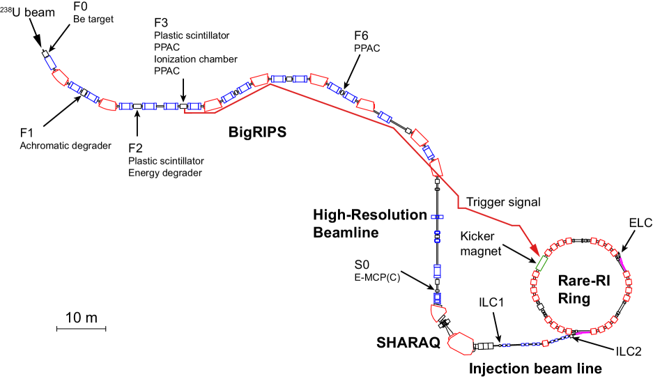
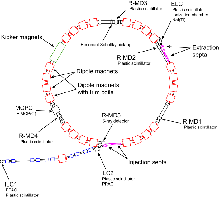
A schematic layout of the Rare-RI Ring and the detector configuration used in the discussed experiment are shown in Figs. 1 and 2. The Rare-RI Ring is placed downstream of a long-injection beamline starting from the production target at F0 and consisting of the high-acceptance multi-stage fragment separator BigRIPS [45], the high-resolution beamline [46], the SHARAQ spectrometer [46, 47], and the injection beam line of the Rare-RI Ring itself. The long-injection beamline is mandatory to achieve the individual-ion injection [42] simultaneously with its precise measurement at resolution.
The Rare-RI Ring consists of six sectors, each of which has four dipole magnets. To achieve the isochronous ion optical setting, two dipole magnets on both ends of each sector are equipped with ten independent single-turn trim coils. Isochronism on the order of can be achieved by adjusting the currents in the trim coils.
Because the Rare-RI Ring is coupled to a cyclotron, the injection of a quasicontinuous beam from a cyclotron into the ring is not compatible. A particle-by-particle injection method into the ring, the so-called individual-ion injection method [42], was established. For its realization, a fast response kicker system [49] was developed. The trigger signal for the kicker system is generated by an ion of interest in the plastic scintillator at the focal plane F3; see Fig. 1. To excite the kicker magnets before the arrival of the ion, the signal is transferred to the kicker system using a high-speed coaxial tube [50]. The achieved signal propagation speed was % of the speed of light. Then, a thyratron switch promptly excites the kicker magnets. We adopted traveling-wave-type kicker magnets to generate a high magnetic field amplitude with a short rise time.
The momentum acceptance of the Rare-RI Ring is designed to be %. The transverse acceptances are and mm mrad in the horizontal and vertical planes, respectively. The residual gas pressure in the Rare-RI Ring ranges from to Pa achieved without baking. Although the pressure is not at ultrahigh vacuum level, it is sufficient to store particles for approximately turns.
IV First demonstration of mass measurement
The first mass measurement of exotic nuclei was performed on five fully stripped nuclei, namely 79As, 78Ge, 77Ga, 76Zn, and 75Cu, all of which have well-known masses tabulated in the Atomic Mass Evaluation, AME2020 [53]. 78Ge was chosen to be the reference particle for tuning the beam transport and isochronous ion optics of the ring. The masses, revolution times, and time-of-flights (TOFs) between F3 and S0 of 79As, 78Ge, 77Ga, and 76Zn were used to fix the parameters for the velocity and magnetic rigidity determination, which is further detailed below. Subsequently, the mass of 75Cu was obtained relative to the mass and revolution time of 78Ge.
The procedure for determining the mass at the Rare-RI Ring is divided into the following five steps: (1) production of RIs; (2) injection of RIs into the ring; (3) circulation confirmation of RIs in the ring; (4) fine-tuning of the isochronous optical setting; (5) storage for several thousands of turns and extraction of RIs. The timing signals at the injection and extraction provide the total TOF.
IV.1 RIs production and events selection
Exotic nuclei near 78Ge were produced via in-flight fission of 238U beams impinging at an energy of 345 MeV/nucleon on a -mm-thick 9Be target. Fission fragments have a large momentum spread of several percent and only a small fraction of them could be transported and injected into the ring. By considering an additional momentum-broadening effect in degraders and detectors mounted in BigRIPS, a momentum slit at the dispersive focal plane F1 of the BigRIPS was set to mm, corresponding to % in momentum.
Standard particle separation was achieved by a combined analysis of the magnetic rigidity and energy loss in the degraders. In this experiment, the magnetic rigidity of the BigRIPS was adjusted to enhance the purity of 78Ge, which was approximately 40% at F3. A wedge-shaped achromatic degrader made of 5-mm-thick aluminum was inserted at F1. A slit with a mm opening at the achromatic focal plane F2 was used to remove undesired contaminants. An additional energy degrader made of -mm-thick aluminum placed at F2 was used for fine tuning the energy of the fragments. The beam energy of 78Ge at F3 was approximately 175 MeV/nucleon.
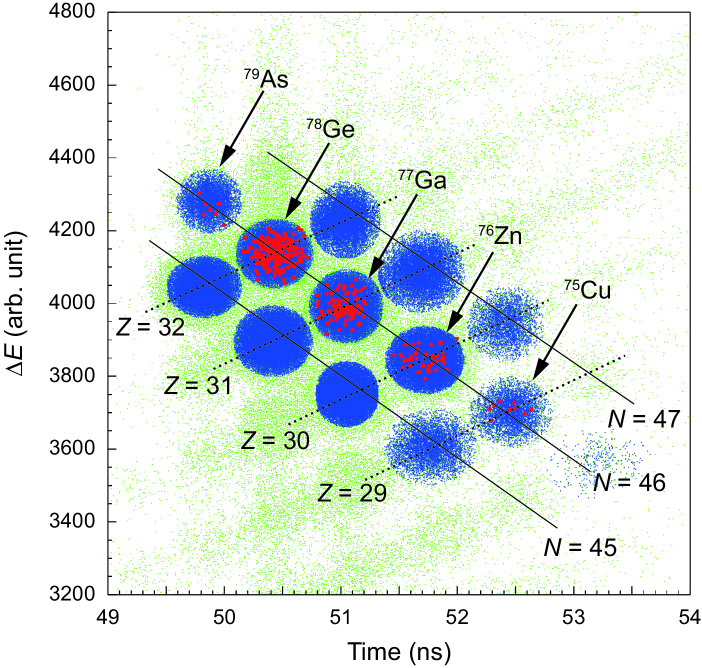
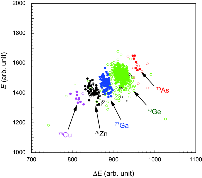
The energy deposit in the ionization chamber at F3 and the TOF between F2 and F3 were measured for particle identification. A typical particle-identification plot is presented in Fig. 3. All the nuclei which generate the trigger signal are indicated by the green dots. To select the valid events, a Gaussian fitting was applied to the and TOF spectra. In this analysis, the selection gates of standard deviations were applied for both the and TOF spectra, as indicated by the blue symbols in Fig. 3.
IV.2 Injection of RIs into the ring
The fission fragments identified at F3 were transported to the ring via the long-injection beamline. Several detectors were placed along it for beam diagnostics. The momenta of the nuclei of interest were measured at the dispersive focal plane F6 of the BigRIPS by using a position-sensitive parallel-plate avalanche counter (PPAC) [54]. The momentum dispersion at F6 () was measured in this experiment to be mm/%.
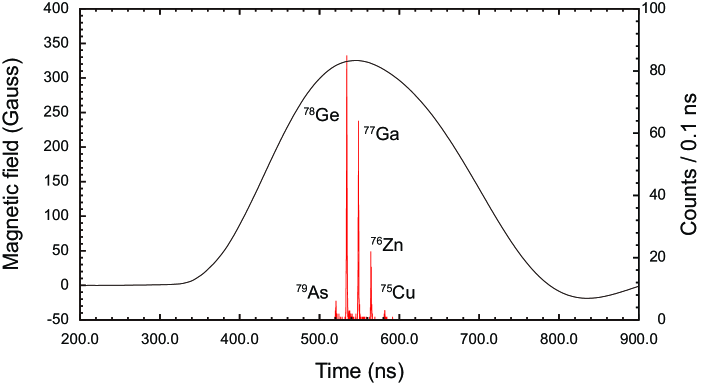
Afterwards, the fission fragments passed through the septum magnets and arrived at the kicker magnets. After the accomplishment of the beam tuning, the detectors placed in the long-injection beamline were removed, except for those placed at F2, F3, F6, and S0. The fission fragments were then individually injected into the ring utilizing the fast-response kicker system [49]. The flight time of the ions from F3 to the kicker was approximately 1 s. The magnetic field of the kicker reached a flat top 950 ns after the trigger signal was generated at F3. This includes the time delays needed for the signal propagation from F3 to the kicker, internal kicker electronic processing, and the response of the magnet itself. To synchronize the particle arrival and the excitation of the magnetic field, an additional 50 ns delay was implemented. A typical waveform of the kicker magnetic field and a histogram of arrival times of the ions of interest at R-MD4 are shown in Fig. 4. As a result, the entire range of the ions of interest could be injected in a single optimized timing setting.
IV.3 Confirmation of circulation of RIs
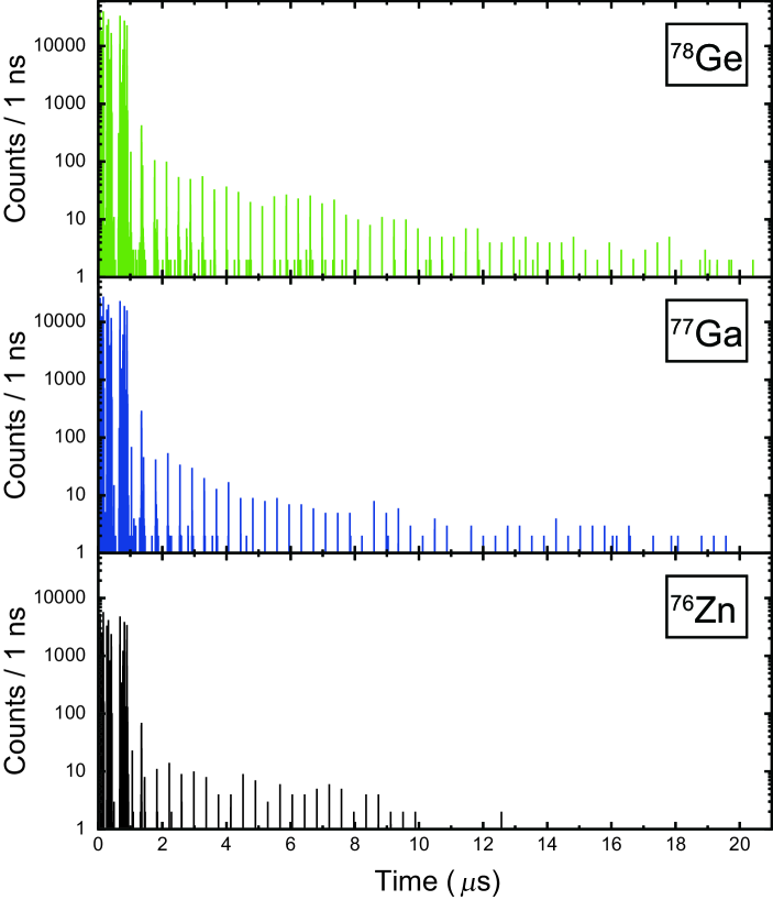
Since only a single ion is injected at a time, standard beam diagnostics is insufficiently sensitive. The first challenge is to control whether an injected particle is revolving in the ring. The circulation of the stored particles was confirmed using an in-ring TOF detector, termed E-MCP, equipped with a carbon foil [E-MCP(C)] [48] placed at MCPC; see Fig. 2. The obtained time spectra of 78Ge, 77Ga, and 76Zn are shown in Fig. 5. The observed periodic time signals indicate that particle circulation was successfully achieved. Stored 78Ge ions circulated for about 60 turns.
The corresponding revolution times were obtained through the analysis described in detail in Ref. [48]. The results are presented in Table 1. The amounts of 79As and 75Cu were insufficient for deducing their revolution times directly. Nevertheless, the revolution times for 79As and 75Cu can be deduced using Eq. (3) and 78Ge as reference. In this analysis, the values of 79As, 75Cu, and 78Ge can be calculated by taking the magnetic rigidity of Tm as measured by an NMR probe located in the ring. The calculated revolution times for 79As and 75Cu are also presented in Table 1. After the circulation of the ions in the ring was confirmed, the destructive E-MCP(C) was removed from the ring aperture.
| RI | Measured revolution time (ns) | Calculated revolution time (ns) |
|---|---|---|
| 79As | 368.404 | |
| 78Ge | 373.121(2) | |
| 77Ga | 378.192(3) | |
| 76Zn | 383.615(5) | |
| 75Cu | 389.448 |
IV.4 Fine-tuning of the isochronous ion optics
The quality of the isochronous ion optics is decisive for mass determination in isochronous mass spectrometry. The optics is extremely sensitive to the applied magnetic fields and their quality. The currents of the trim coils incorporated into the dipole magnets of the ring were tuned to obtain the required magnetic-field distribution. The magnetic field setting was optimized for the reference particle, 78Ge, by monitoring the correlation between the TOF from S0 to ELC (TOFS0ELC) and the particle momentum, which was measured at F6 prior to the injection into the ring. If isochronous ion optics is perfectly optimized for the reference particle 78Ge, the TOFS0ELC(78Ge) will be constant and independent of momentum. Thus, the quality of the isochronous ion optics is quantified by the momentum dependence on TOFS0ELC(78Ge). In this experiment, second-order ion-optical tuning was adopted.
Green symbols in Fig. 6 demonstrate the momentum dependence of the TOFS0ELC of 78Ge reference particles. In this figure, the abscissa axis is the momentum () deviation from the momentum at a weighted average position at F6 (), . The momentum deviation was calculated using the position information of the events at F6 (), the weighted average of () described in Sec. V.2, and the momentum dispersion at F6 () as . The E-MCP(C) at S0 and the plastic scintillator at ELC were used to measure TOFS0ELC. Owing to the second-order tuning of the magnetic fields, a small third-order dependence appeared in the correlation between TOFS0ELC(78Ge) and the momentum. A precision of TOFS0ELC(78Ge) was achieved to be ppm (standard deviation) for a momentum spread of %.
IV.5 Storage and extraction of RIs and TOF measurement
After a defined storage time, the particles were extracted from the ring using the same kicker magnets and the same magnetic field distribution as the one used for the injection. Two storage-time intervals were set, namely s to extract 79As, 78Ge, 77Ga, and 75Cu, and s for 76Zn.
Total flight time TOFS0ELC spectra are shown in Fig. 6. In contrast to the TOFS0ELC of 78Ge, momentum dependences are clearly observed in TOFS0ELC for 79As, 77Ga, 76Zn, and 75Cu. The TOFS0ELC of approximately 0.7 ms was used instead of measuring revolution times in the ring turn by turn. The latter would be advantageous, but the corresponding detector needs to be non-destructive, which remains a challenge. The previously discussed E-MCP(C) counter introduces energy losses in the carbon foil, which limits the particle storage to only a few tens of turns, whereas about 2000 revolutions are needed to achieve the anticipated mass precision.
The number of turns for each particle was determined using the revolution time and the time interval between injection and extraction. The obtained turn numbers are listed in Table 2. In the mass determination, the listed turn numbers were incremented by 2 in consideration that the sum of the flight path lengths from S0 to the kicker and from the kicker to ELC is approximately twice the ring circumference.
A long-range time-to-digital converter (Acqiris TC842 [55]) was used to measure the total TOFS0ELC defined by the start signal from the E-MCP(C) at S0 and the stop signal from the plastic scintillator at ELC. The signals from the E-MCP(C), plastic scintillator, and the trigger detector were processed through a constant fraction discrimination (Ortec935 [56]) before being fed into the Acqiris TC842.
| RI | Number of turns |
|---|---|
| 79As | 1902 |
| 78Ge | 1878 |
| 77Ga | 1853 |
| 76Zn | 1826 |
| 75Cu | 1799 |
V Mass determination
To determine using Eqs. (4) and (6), the revolution times and the velocity or magnetic rigidity need to be known. The revolution times were calculated using the corresponding TOFS0ELC and . Since can be corrected by using either or , there are two analytical methods for determining .
V.1 Extracted events selection
As described in Sec. IV.1, the fission fragments were identified at F3 prior to injection. Furthermore, the fragments were also identified at ELC as successfully extracted events. The extracted events were defined as those that had proper TOF stop data from the plastic scintillator at ELC. In addition, events were selected from a particle identification at ELC using the total energy and information obtained by the NaI(Tl) counter and ionization chamber, respectively, as shown in Fig 7. The selection gates of and standard deviations were applied to both the and spectra, respectively. The selected valid extraction events obtained in a 3-hour-accumulation period are plotted and indicated by the red dots in Fig. 3. The number of selected extraction events is listed in Table 3.
| RI | Number of events |
|---|---|
| 79As | |
| 78Ge | |
| 77Ga | |
| 76Zn | |
| 75Cu |
V.2 Velocity determination
Absolute values of velocity are crucial for correcting via Eq. (4). Each value was calculated employing TOF from F3 to S0, TOFF3S0, as:
| (9) |
where is the flight path length between F3 and S0, and is the offset of the measured TOFF3S0. To obtain and , we assume that the velocities between F3 and S0, , and between S0 and ELC, , are the same. Thus, the following equations hold:
| (10) | ||||
where m is the flight length in the ring, see Sec. V.3. To obtain the precise velocities, we used momentum-corrected TOFF3S0-cor and instead of TOFF3S0 and in Eq. (10) using the following equations:
| (11) | ||||
where () denotes the slope of the TOFF3S0–position(momentum) (–position) correlation. The slopes of the correlations were obtained by a fitting analysis using a first-order polynomial. An example of the correlation plot of for 76Zn is shown by the black filled circles in Fig. 8. The momentum dependence of is clearly seen and can be corrected accordingly. The corrected , , is indicated by the black open circles in Fig. 8. The momentum dependence was sufficiently reduced through this procedure. The same analysis was performed for 79As, 78Ge, 77Ga, and 76Zn.
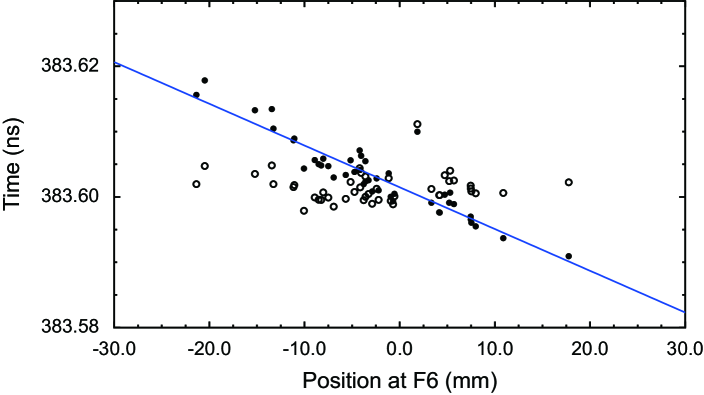
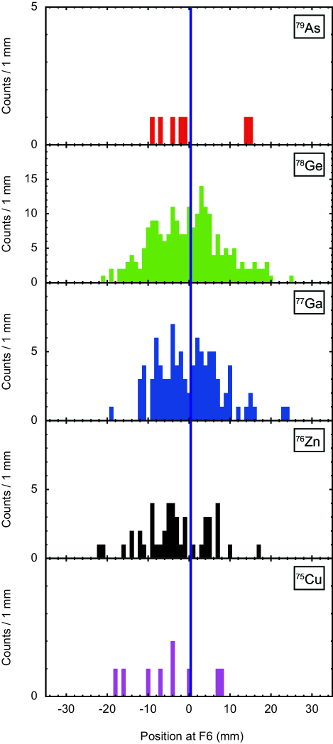
Figure 9 depicts the position distributions for each stored nuclear species at the dispersive focal plane F6. The weighted average position, mm, is indicated by the blue line in Fig. 9, which was obtained by considering the weighted average of the individual weighted average positions of 79As, 78Ge, 77Ga, and 76Zn.
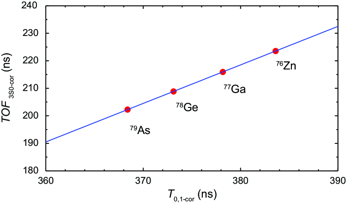
and were determined through a linear fit according to Eq. (10) of the correlation plot between TOFF3S0-cor and , as shown in Fig. 10. The uncertainties of TOFF3S0-cor were about 0.3 to 1.6 ps, while the fit residua [TOFTOF] were within ps. The resultant and values are m and ns. The values of 75Cu were calculated event-by-event using Eq. (9) adopting the measured TOFF3S0, flight length , and offset .
Based on the principle of mass measurement, of 75Cu should coincide with . However, the experimental of 75Cu exhibited a small difference. Possible reasons for this disagreement may be the momentum-dependent flight path lengths and energy losses in the PPAC at F6, which could not be accurately considered. These effects are sources of systematic uncertainties. To account for them, we introduced a correction factor for of 75Cu to match . The correction factor is defined as the ratio at . To obtain the ratio , the experimental and as a function of the F6 position were fitted using the first-order polynomial, as shown in Fig. 11. The fit results of the values at the F6 weighted average position were used to calculate the ratio giving for 75Cu. The final taken for the mass determination was obtained via .
V.3 Magnetic rigidity determination
The absolute magnetic rigidities of each particle are crucial for correcting via Eq. (6). The magnetic rigidities were not directly measured for each event and were thus calculated using the following equation:
| (12) |
where is the mean value of the magnetic rigidity of the ring, is the F6 position, is the weighted average position at F6, and mm/ is the dispersion measured at F6.
Based on the definition of magnetic rigidity, the relationship between (u/) and is:
| (13) |
where u and denote the unified atomic mass unit, and velocity, respectively. The velocity, respectively can be expressed as with a flight length and time-of-flight . Hence, the relationship between and is obtained:
| (14) |
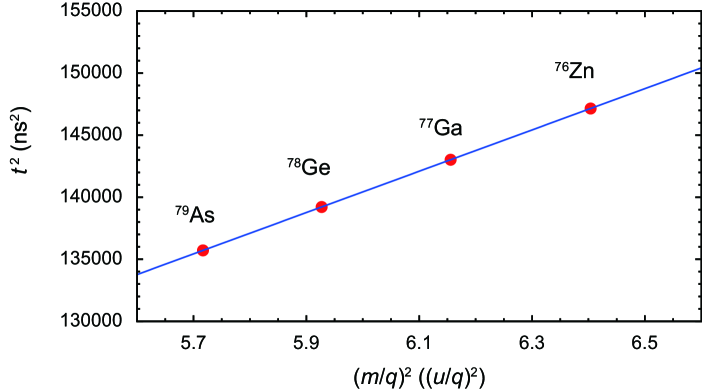
To evaluate , the momentum-corrected revolution times and the mean ring circumference are taken as and , respectively, in Eq. (14). Figure 12 presents as a function of the squared mass-to-charge ratio from AME2020 [53]. A linear fitting analysis using Eq. (14) provided and as free parameters. Consequently, and were obtained to be Tm and m. Whereas the uncertainties of the data points are about 0.1 to 0.3 ns2, the corresponding uncertainties of the fit residua [] are as small as ns2. The obtained magnetic field in the analysis was different from that measured by the NMR probe in the ring described in Sec. IV.3. This difference could be attributed to the fact that the NMR probe in the ring was not installed at a position corresponding to the momentum at . The magnetic rigidities of each particle were determined through Eq. (12).
V.4 Revolution times in the Rare-RI Ring
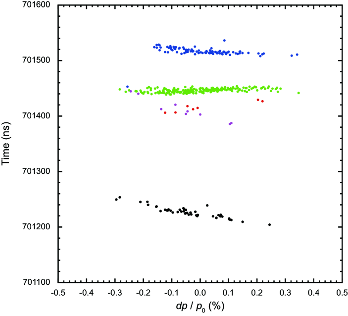
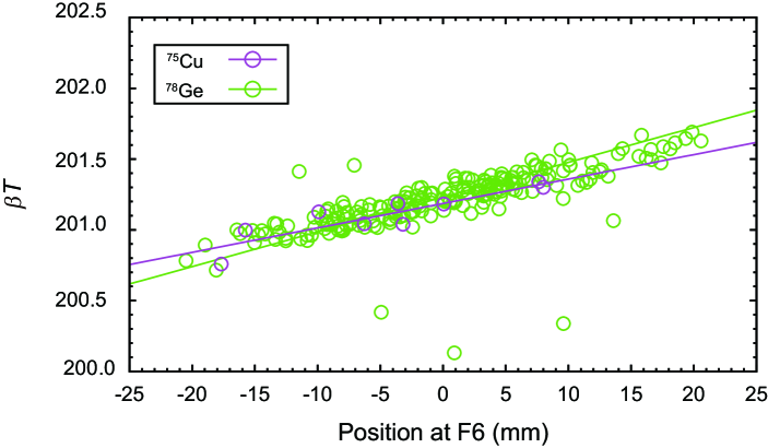
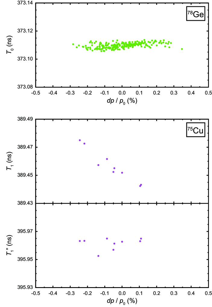
The revolution times obtained for 78Ge and 75Cu are shown in Fig. 13 as a function of the momentum measured at F6. Because isochronism is fulfilled for the reference 78Ge, the momentum dependence of of 78Ge is not observed; however, that of 75Cu is apparent and can be corrected using or . Figure 13 (bottom) presents , which is corrected by . The mean value was ns, and the mean value was ns. Therefore, the uncertainty of is on the order of and that of is on the order of . The uncertainty of mainly stems from the magnetic field instabilities and time resolutions of the timing detectors at S0 and ELC.
V.5 Masses
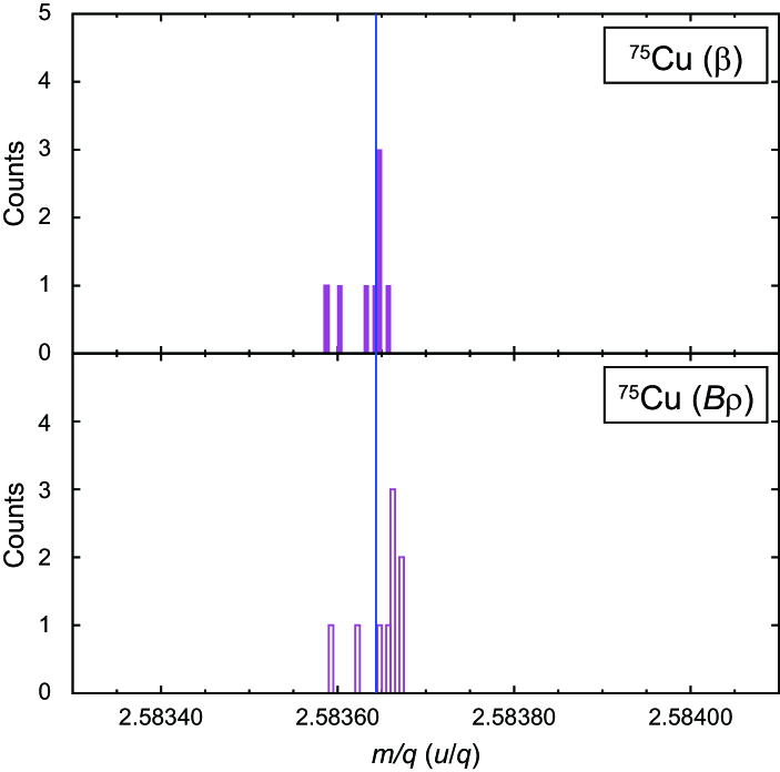
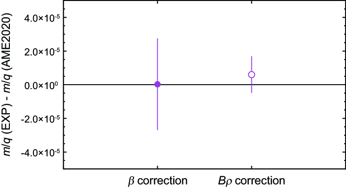
The values were evaluated for each event by adopting the corresponding , , and in Eqs. (4) and (6). In the analyses, a constant value of ns was used. Because the mass of 75Cu is well known, comparing the obtained experimental values to the literature values from AME2020 [53] allows the verification of the present mass determination procedure. Figure 14 presents the spectra of 75Cu obtained using the and corrections. The value u/ was obtained by employing the correction and u/ by employing the correction. Figure 15 presents a comparison of the experimental values with the literature value [ u/]. The differences between the experimental and literature values is less than u/. The mass excess () values obtained in these measurements are 54460(740) keV and 54310(290) keV, while the literature mass excess value is 54470.2(7) keV [53].
The total uncertainty for the correction analysis was deduced via
| (15) |
where is the statistical uncertainty of , and , , and are propagated statistical uncertainties from , , and corrections, respectively. For the correction analysis, the total uncertainty is given as
| (16) |
where , , and are the uncertainties due to the error propagation from , , and , respectively. Because the relative uncertainty of is negligible (), we neglected this contribution in the analyses.
The statistical uncertainties of values were obtained using the standard deviation, , of the distribution and the number of events, , using the equation . These uncertainties were deduced to be u/ and u/ for the and corrections, respectively. The time fluctuations of the ring magnetic field change the time-of-flight in the ring and broaden the peak width of the spectrum. As a result, it affects the statistical uncertainty of .
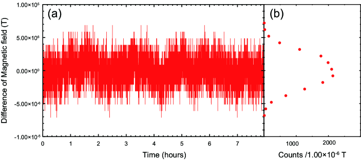
Figure 16 (a) presents the typical time fluctuations of the magnetic field of a dipole magnet during the measurement period. The magnitude of the fluctuation shown in Fig. 16 (b) was estimated to be T (standard deviation), while the average magnetic field was 1.2035462 T. A momentum dependence of the and values also affects the statistical uncertainty of . As shown in Fig. 13(bottom), the momentum dependence of the value remained observable. This dependence arises from the inaccurately known or .
The uncertainty of depends on the quality of isochronous optics and timing resolution of the detectors. The main contribution to the uncertainty of stems from the optics imperfections, because the time resolution of the detectors was on the order of several tens of ps. The uncertainties were deduced to be u/ and u/ for the and corrections, respectively. The uncertainties of , , , , and depend on the statistics and fitting procedure. The contributions of each uncertainty and the total uncertainties are listed in Table 4.
The total obtained uncertainties were u/ and u/ for the and correction approaches, respectively. These values correspond to keV and keV. These uncertainties are about 10 times larger than the uncertainties of the upgraded isochronous mass measurements in CSRe [37, 39, 40], but comparable to the uncertainties of the original isochronous mass measurements in ESR [28, 27, 57].
Significant contributions to the total uncertainties were due to the statistical uncertainty of and uncertainty arising from the correction factor in the correction procedure. For the correction routine, the statistical uncertainty was the main contributor to the total uncertainty. These results suggest that the improvement in the instabilities of the magnetic fields and the determination of accurate and values are essential. In this study, simple methods to obtain and were adopted. However, the analysis can be further improved to obtain more accurate and/or .
| Contribution | (u/) | (u/) |
|---|---|---|
| – | ||
| – | ||
| – | ||
| – | ||
| – | ||
VI Conclusion
This study describes the first isochronous mass spectrometry implemented in the Rare-RI Ring, which was conducted on nuclei with well-known masses and preceded the first mass measurements of new results reported in Ref. [43]. Individual-ion injection method, ion injection, storage, and extraction, together with TOF measurements in the ring applied to exotic nuclei have successfully been achieved. Consequently, the known mass of 75Cu was re-measured under the strict conditions of short measurement durations. The measurement time of approximately 0.7 ms is excellently suited for pinning down yet unmeasured masses of the most exotic nuclei.
We established two analytical methods for the mass determination employing either or corrections. The obtained mass accuracies and uncertainties were on the order of the u/ and u/, respectively for both, and , correction methods. The major sources of the total uncertainty for the correction analysis were the statistical uncertainty of and the uncertainty of ; whereas for the correction analysis, it was the statistical uncertainty of . The instabilities of the magnetic fields of the Rare-RI Ring and the momentum dependence of affected the statistical uncertainty of the value. This study suggests further improvements of the stability of the magnetic fields of the Rare-RI Ring to facilitate more accurate determination of and values.
Nonetheless, the obtained mass of 75Cu is in satisfactory agreement with the literature value. The Rare-RI Ring facility has proved to be a powerful tool for mass measurements of rare RIs. Following the first results reported in [43], the Rare-RI Ring will be used for further mass measurements of short-lived nuclei, especially for nuclei involved in the process.
VII Acknowledgments
The authors thank the accelerator staff of RIKEN Ring Cyclotron for support during the experiment. This experiment on the Rare-RI Ring was performed at the RI beam factory operated by RIKEN Nishina Center and CNS, University of Tokyo under the Experimental Program MS-EXP16-10. This work was supported by the RIKEN Pioneering Project funding and JSPS KAKENHI Grants No. 26287036, No. 25105506, No. 15H00830, and No. 17H01123. YAL received funding from the European Research Council (ERC) under the European Union’s Horizon 2020 research and innovation programme (Grant Agreement No. 682841 “ASTRUm”).
References
- T. Yamaguchi et al. [2021] T. Yamaguchi et al., Masses of exotic nuclei, Progress in Particle and Nuclear Physics 120, 103882 (2021).
- John J. Cowan et al. [2021] John J. Cowan et al., Origin of the heaviest elements: The rapid neutron-capture process, Reviews of Modern Physics 93, 015002 (2021).
- C.J. Horowitz et al. [2019] C.J. Horowitz et al., r-process nucleosynthesis: connecting rare-isotope beam facilities with the cosmos, Journal of Physics G: Nuclear and Particle Physics 46, 083001 (2019).
- Darach Watson et al. [2019] Darach Watson et al., Identification of strontium in the merger of two neutron stars, Nature 574, 497 (2019).
- B.P. Abbott et al. [2017a] B.P. Abbott et al., Multi-messenger Observations of a Binary Neutron Star Merger, The Astrophysical Journal Letters 848, L12 (2017a).
- M. R. Drout et al. [2017] M. R. Drout et al., Light curves of the neutron star merger GW170817/SSS17a: Implications for r-process nucleosynthesis, Science 358, 1570 (2017).
- B.P. Abbott et al. [2017b] B.P. Abbott et al. (LIGO Scientific Collaboration and Virgo Collaboration), GW170817: Observation of Gravitational Waves from a Binary Neutron Star Inspiral, Phys. Rev. Lett. 119, 161101 (2017b).
- B. Sun et al. [2008a] B. Sun et al., Application of the relativistic mean-field mass model to the -process and the influence of mass uncertainties, Physical Review C 78, 025806 (2008a).
- D. Martin et al. [2016] D. Martin et al., Impact of Nuclear Mass Uncertainties on the Process, Physical Review Letters 116, 121101 (2016).
- X.F. Jiang et al. [2021] X.F. Jiang et al., Sensitivity Study of r-process Abundances to Nuclear Masses, The Astrophysical Journal 915, 29 (2021).
- Jens Dilling et al. [2018] Jens Dilling et al., Penning-Trap Mass Measurements in Atomic and Nuclear Physics, Annual Review of Nuclear and Particle Science 68, 45 (2018).
- G. Bollen [1997] G. Bollen, Radioactive Ion Beams and Penning Traps, Nuclear Physics A 616, 457c (1997).
- J. Dilling et al. [2000] J. Dilling et al., The SHIPTRAP project: A capture and storage facility at GSI for heavy radionuclides from SHIP, Hyperfine Interactions 127, 491 (2000).
- V.S. Kolhinen et al. [2004] V.S. Kolhinen et al., JYFLTRAP: a cylindrical Penning trap for isobaric beam purification at IGISOL, Nuclear Instruments and Methods in Physics Research Section A 528, 776 (2004).
- R. Ringle et al. [2006] R. Ringle et al., Precision mass measurements with LEBIT at MSU, International Journal of Mass Spectrometry 251, 300 (2006).
- R.N. Wolf et al. [2013] R.N. Wolf et al., ISOLTRAP’s multi-reflection time-of-flight mass separator/spectrometer, International Journal of Mass Spectrometry 349-350, 123 (2013).
- P. Schury et al. [2014] P. Schury et al., A high-resolution multi-reflection time-of-flight mass spectrograph for precision mass measurements at RIKEN/SLOWRI, Nuclear Instruments and Methods in Physics Research B 335, 39 (2014).
- W.R. Pla et al. [2013] W.R. Pla et al., The FRS Ion Catcher - A facility for high-precision experiments with stopped projectile and fission fragments, Nuclear Instruments and Methods in Physics Research B 317, 457 (2013).
- Christian Jesch et al. [2015] Christian Jesch et al., The MR-TOF-MS isobar separator for the TITAN facility at TRIUMF, Hype. Int. 235, 97 (2015).
- Yu.A. Litvinov et al. [2005] Yu.A. Litvinov et al., Mass measurement of cooled neutron-deficient bismuth projectile fragments with time-resolved Schottky mass spectrometry at the FRS-ESR facility, Nuclear Physics A 756, 3 (2005).
- M. Hausmann et al. [2000] M. Hausmann et al., First isochronous mass spectrometry at the experimental storage ring ESR, Nuclear Instruments and Methods in Physics Research Section A 446, 569 (2000).
- M. Hausmann et al. [2001] M. Hausmann et al., Isochronous Mass Measurements of Hot Exotic Nuclei, Hyperfine Interactions 132, 289 (2001).
- X.L. Tu et al. [2011] X.L. Tu et al., Precision isochronous mass measurements at the storage ring CSRe in Lanzhou, Nuclear Instruments and Methods in Physics Research Section A 654, 213 (2011).
- S. Baruah et al. [2008] S. Baruah et al., Mass Measurements beyond the Major -Process Waiting Point , Physical Review Letters 101, 262501 (2008).
- B. Sun et al. [2008b] B. Sun et al., Nuclear structure studies of short-lived neutron-rich nuclei with the novel large-scale isochronous mass spectrometry at the FRS-ESR facility, Nuclear Physics A 812, 1 (2008b).
- D. Atanasov et al. [2015] D. Atanasov et al., Precision Mass Measurements of 129-131Cd and Their Impact on Stellar Nucleosynthesis via the Rapid Neutron Capture Process, Physical Review Letters 115, 232501 (2015).
- R. Kn̈obel et al. [2016] R. Kn̈obel et al., First direct mass measurements of stored neutron-rich 129,130,131Cd isotopes with FRS-ESR, Physics Letters B 754, 288 (2016).
- R. Kn̈obel et al. [2016] R. Kn̈obel et al., New results from isochronous mass measurements of neutron-rich uranium fission fragments with the FRS-ESR-facility at GSI, The European Physical Journal A 52, 138 (2016).
- M. Vilen et al. [2018] M. Vilen et al., Precision Mass Measurements on Neutron-Rich Rare-Earth Isotopes at JYFLTRAP: Reduced Neutron Pairing and Implications for -Process Calculations, Physical Review Letters 120, 262701 (2018).
- Y. Yano [2007] Y. Yano, The RIKEN RI Beam Factory Project: A status report, Nuclear Instruments and Methods in Physics Research Section B 261, 1009 (2007).
- A. Ozawa et al. [2012] A. Ozawa et al., The rare-RI ring, Progress of Theoretical and Experimental Physics 2012, 03C009 (2012).
- B. Franzke [1987] B. Franzke, The heavy ion storage and cooler ring project ESR at GSI, Nuclear Instruments and Methods in Physics Research Section B 24/25, 18 (1987).
- [33] The heavy ion cooler-storage-ring project (HIRFL-CSR) at Lanzhou, Nuclear Instruments and Methods in Physics Research Section A”, volume = ”488”, pages = ”11–25”, year = ”2002”, author = ”J.W. Xia et al.”, doi = ”https://doi.org/10.1016/S0168-9002(02)00475-8” .
- Markus Steck and Yuri A. Litvinov [2020] Markus Steck and Yuri A. Litvinov, Heavy-ion storage rings and their use in precision experiments with highly charged ions, Progress in Particle and Nuclear Physics 115, 103811 (2020).
- H. Geissel and Yu.A. Litvinov [2005] H. Geissel and Yu.A. Litvinov, Precision experiments with relativistic exotic nuclei at GSI, Journal of Physics G: Nuclear and Particle Physics 31, S1779 (2005).
- H. Geissel et al. [2006] H. Geissel et al., A new experimental approach for isochronous mass measurements of short-lived exotic nuclei with the FRS-ESR facility, Hyperfine Interactions 173, 49 (2006).
- M. Wang et al. [2022] M. Wang et al., -defined isochronous mass spectrometry: An approach for high-precision mass measurements of short-lived nuclei, Phys. Rev. C 106, L051301 (2022).
- H. Geissel et al. [2023] H. Geissel et al., Novel isochronous features for FRS-ESR experiments with stored exotic projectile fragments, Nuclear Instruments and Methods in Physics Research Section B 541, 305 (2023).
- M. Zhang et al. [2023] M. Zhang et al., B-defined isochronous mass spectrometry and mass measurements of 58Ni fragments, The European Physical Journal A 59, 27 (2023).
- X. Zhou et al. [2023] X. Zhou et al., Mass measurements show slowdown of rapid proton capture process at waiting-point nucleus 64Ge, Nature Physics (2023).
- M. Wang et al. [2023] M. Wang et al., Mass Measurement of Upper -Shell and Nuclei and the Importance of Three-Nucleon Force along the Line, Physical Review Letters 130, 192501 (2023).
- I. Meshkov et al. [2004] I. Meshkov et al., Individual rare radioactive ion injection, cooling and storage in a ring, Nuclear Instruments and Methods in Physics Research Section A 523, 262 (2004).
- H.F. Li et al. [2022] H.F. Li et al., First Application of Mass Measurements with the Rare-RI Ring Reveals the Solar -Process Abundance Trend at and , Physical Review Letters 128, 152701 (2022).
- Y.H. Zhang et al. [2016] Y.H. Zhang et al., Storage ring mass spectrometry for nuclear structure and astrophysics research, Physica Scripta 91, 073002 (2016).
- Toshiyuki Kubo [2003] Toshiyuki Kubo, In-flight RI beam separator BigRIPS at RIKEN and elsewhere in Japan, Nuclear Instruments and Methods in Physics Research Section B 204, 97 (2003).
- S. Michimasa et al. [2013] S. Michimasa et al., SHARAQ spectrometer for high-resolution studies for RI-induced reactions, Nuclear Instruments and Methods in Physics Research Section B 317, 305 (2013).
- T. Uesaka et al. [2008] T. Uesaka et al., The high resolution SHARAQ spectrometer, Nuclear Instruments and Methods in Physics Research Section B 266, 4218 (2008).
- D. Nagae et al. [2021] D. Nagae et al., Development and operation of an electrostatic time-of-flight detector for the Rare RI storage Ring, Nuclear Instruments and Methods in Physics Research Section A 986, 164713 (2021).
- H. Miura et al. [2015] H. Miura et al., Performance of a Fast Kicker Magnet for Rare-RI Ring, Part of Proceedings, 13th Heavy Ion Accelerator Technology Conference (HIAT2015) , MOPA23 (2015).
- Shunichiro Omika et al. [2021] Shunichiro Omika et al., Development of Experimental Devices for Precise Mass Measurements at the Rare-RI Ring Facility, JPS Conference Proceedings 35, 011026 (2021).
- S. Omika et al. [2020] S. Omika et al., Development of a new in-ring beam monitor in the Rare-RI Ring, Nuclear Instruments and Methods in Physics Research Section B 463, 241 (2020).
- F. Suzaki et al. [2013] F. Suzaki et al., Design study of a resonant Schottky pick-up for the Rare-RI Ring project, Nuclear Instruments and Methods in Physics Research Section B 317, 636 (2013).
- Meng Wang et al. [2021] Meng Wang et al., The AME 2020 atomic mass evaluation (II). Tables, graphs and references, Chinese Physics C 45, 030003 (2021).
- H. Kumagai et al. [2013] H. Kumagai et al., Development of Parallel Plate Avalanche Counter (PPAC) for BigRIPS fragment separator, Nuclear Instruments and Methods in Physics Research Section B 317, 717 (2013).
- [55] Acqiris - Time-to-Digital Converter TC842, .
- [56] ORTEC - Quad Constant-Fraction 200-MHz Discriminator 935, .
- J. Stadlmann et al. [2004] J. Stadlmann et al., Direct mass measurement of bare short-lived 44V, 48Mn, 41Ti and 45Cr ions with isochronous mass spectrometry, Physics Letters B 586, 27 (2004).