Multi-label Learning with Random Circular Vectors

Abstract

The extreme multi-label classification (XMC) task involves learning a classifier that can predict from a large label set the most relevant subset of labels for a data instance. While deep neural networks (DNNs) have demonstrated remarkable success in XMC problems, the task is still challenging because it must deal with a large number of output labels, which make the DNN training computationally expensive. This paper addresses the issue by exploring the use of random circular vectors, where each vector component is represented as a complex amplitude. In our framework, we can develop an output layer and loss function of DNNs for XMC by representing the final output layer as a fully connected layer that directly predicts a low-dimensional circular vector encoding a set of labels for a data instance. We conducted experiments on synthetic datasets to verify that circular vectors have better label encoding capacity and retrieval ability than normal real-valued vectors. Then, we conducted experiments on actual XMC datasets and found that these appealing properties of circular vectors contribute to significant improvements in task performance compared with a previous model using random real-valued vectors, while reducing the size of the output layers by up to 99%.

1 Introduction

Extreme multi-label classification (XMC) problems arise in various domains, such as product recommendation systems Jain et al. (2016), labeling large encyclopedia Dekel and Shamir (2010); Partalas et al. (2015), instance-level image recognition Deng et al. (2010); Ridnik et al. (2021) and natural language generation Mikolov et al. (2013). The XMC task involves learning a classifier which can predict from a large label set the most relevant subset of labels for a data instance. Recent work has focused on deep neural network (DNN) models (Liu et al., 2017; You et al., 2019; Chang et al., 2020; Zhang et al., 2021; Dahiya et al., 2023; Jain et al., 2023) that deliver task performances superior to those of early approaches using linear predictors (Babbar and Schölkopf, 2017; Prabhu et al., 2018b).

While DNN models have brought great performance improvements, the XMC task still remains a challenge mainly due to the extremely large output space. Since a large number of output labels make it difficult to train DNN models efficiently, various methods for improving training efficiency have been proposed (Khandagale et al., 2020; Wydmuch et al., 2018; Jiang et al., 2021; Ganesan et al., 2021). Among the previous studies, Ganesan et al. (2021) presented a promising method that employs random real-valued vectors for reducing the output layer size of DNN models. In this approach, a high-dimensional output space vector is replaced with a low-dimensional random vector encoding the relevant label information for a data instance. Then, DNN models are trained to predict the label-encoded vector directly. After the model generates a vector, it can be checked approximately whether a label is encoded in it or not through a vector comparison using the cosine similarity between the output vector and a vector that the label is assigned to. The basic idea of the label encoding and retrieval framework relies on the theory of Holographic Reduced Representations (Plate, 1995), which was developed in the cognitive neuroscience field.

However, random real-valued vectors do not have sufficient ability for representing data instances that belong to many class concepts. As our experiments in § 3 show, the label retrieval accuracy decreases markedly as the number of class labels encoded in a vector increases. To alleviate the issue, this paper presents a novel method that uses circular vectors instead of real-valued vectors. Each element of a circular vector takes a complex amplitude as its value; i.e., the vector element is represented by an angle ranging from $-\pi$ to $\pi$. Since an angle can be represented by a real value, the memory cost for the circular vector representation is the same as that for a normal real-valued vector. In spite of this fact, surprisingly, circular vectors have better label encoding and retrieval capacities than real-valued vectors. One of the challenges in applying circular vectors to DNN models is how to adapt the output layer to a circular vector. In § 4, we describe our neural network architecture that uses circular vectors in the output layer. Our experimental results on XMC datasets show that our method based on circular vectors significantly outperforms a previous model using real-valued vectors, while reducing the size of the output layers by up to 99%.

2 Previous Study: Learning with Holographic Reduced Representations

Several vector symbolic architectures have been developed in the field of cognitive neuroscience, including Tensor Product Representations (Smolensky, 1990), Binary Spatter Code (Kanerva, 1996), Binary Sparse Distributed Representations (Rachkovskij, 2001), Multiply-Add-Permute (Gayler, 2004), and Holographic Reduced Representations (HRR) (Plate, 1995). Among them, HRR is a successful architecture for distributed representations of compositional structures. To model complex structured prediction tasks in a vector space that involve key-value stores, sequences, trees and graphs, many prior studies have explored how to use HRR in various machine learning frameworks; Recurrent Neural Networks (Plate, 1992), Tree Kernels (Zanzotto and Dell’Arciprete, 2012), Knowledge Graph Representation Learning (Nickel et al., 2016; Hayashi and Shimbo, 2017), Long-short Term Memory Networks (Danihelka et al., 2016), Transformer Networks (Alam et al., 2023), and among others. In particular, Ganesan et al. (2021) presented a general framework based on the HRR architecture for efficient multi-label learning of DNN models. To clarify the motivation of our study, we will review the framework in more detail in the following subsections.

2.1 Holographic Reduced Representations (HRR)

In the HRR architecture, terms in a domain are represented by real-valued vectors. Here, we assume that each vector is independently sampled from a Gaussian distribution $\mathcal{N}(0,\mathbf{I}_{d}\cdot d^{-1})$, where $d$ is the vector dimension size and $\mathbf{I}_{d}$ is the $d\times d$ identity matrix. To bind an association of two terms represented by vectors $\mathbf{a}$ and $\mathbf{b}$, respectively, HRR uses circular convolution, denoted by the mathematical symbol $\otimes$:

$$\mathbf{a}\otimes\mathbf{b}=\mathcal{F}^{-1}(\mathcal{F}(\mathbf{a})\odot\mathcal{F}(\mathbf{b}))$$ (1)

where $\odot$ is element-wise vector multiplication. Note that the circular convolution can be computed by using a fast Fourier transform (FFT) $\mathcal{F}$ and inverse FFT $\mathcal{F}^{-1}$, but they require $\mathcal{O}(d\log d)$ computation time. Given several associations $\mathbf{a}\otimes\mathbf{b}$, $\mathbf{c}\otimes\mathbf{d}$ and $\mathbf{e}\otimes\mathbf{f}$, the vectors can be superposed to represent their combination: $\mathbf{S}=(\mathbf{a}\otimes\mathbf{b})\oplus(\mathbf{c}\otimes\mathbf{d})\oplus(\mathbf{e}\otimes\mathbf{f})$, where the “superposition” operator $\oplus$ is just normal vector addition $+$. The HRR architecture also provides the inversion operation ${\dagger}$:

$$\mathbf{a}^{{\dagger}}=\mathcal{F}^{-1}(\frac{1}{\mathcal{F}(\mathbf{a})}).$$ (2)

The inversion operation can be used to perform “unbinding”. For an example, it allows the reconstruction of a noisy version of $\mathbf{d}$ to be recreated from the memory $\mathbf{S}$ and a cue $\mathbf{c}$: $\mathbf{S}\otimes\mathbf{c}^{{\dagger}}\approx\mathbf{d}$. Finally, the “similarity” operation is defined as the dot-product $\mathbf{a}^{\mathrm{T}}\mathbf{b}$. Using the similarity operation, we can check approximately whether $\mathbf{a}$ exists in a memory $\mathbf{S}$ if $\mathbf{S}^{\mathrm{T}}\mathbf{a}\approx 1$ or not present if $\mathbf{S}^{\mathrm{T}}\mathbf{a}\approx 0$.

2.2 Multi-label Learning with HRR

Ganesan et al. (2021) introduced a novel method using HRR for reducing the computational complexity of training DNNs for XMC tasks. Let $L$ be the number of class labels in an XMC task. The basic idea behind the approach of (Ganesan et al., 2021) is quite intuitive; for efficient DNN training, an $L$-dimensional output (teacher) vector is replaced with a $d$-dimensional real-valued vector encoding the relevant label information for a data instance. By assuming $d\ll L$, we can dramatically reduce the output layer size of the DNN model.

In this approach, each class label $y$ is assigned to a $d$-dimensional vector $\mathbf{c}_{y}\in\mathbb{R}^{d}$. Then, the label information for a data instance $x$ is represented as a label vector $\mathbf{S}_{x}\in\mathbb{R}^{d}$:

$$\mathbf{S}_{x}=\bigoplus_{p\in\mathcal{Y}_{x}}\mathbf{p}\otimes\mathbf{c}_{p}$$ (3)

where $\mathcal{Y}_{x}$ denotes the set of class labels that $x$ belongs to and $\mathbf{p}\in\mathbb{R}^{d}$ represents the positive class concept. To train a DNN model $f(\mathbf{x})$ that generates $\hat{\mathbf{S}}_{x}\in\mathbb{R}^{d}\approx\mathbf{S}_{x}$, Ganesan et al. (2021) define a loss function:

$$loss=\sum_{p\in\mathcal{Y}_{x}}(1-sim{((\hat{\mathbf{S}}_{x}\otimes\mathbf{p}^{{\dagger}}),\mathbf{c}_{p}})).$$ (4)

To prevent the model from maximizing the magnitudes of the output vectors, Ganesan et al. (2021) used the cosine similarity as $sim(\cdot,\cdot)$, which is a normalized version of the dot product that ranges from -1 to 1. In the inference phase, labels can also be ranked according to the cosine similarity computed by $sim(\hat{\mathbf{S}}_{x}\otimes\mathbf{p}^{{\dagger}},\mathbf{c}_{p})$ for each label $p$. Moreover, Ganesan et al. (2021) introduced a novel vector projection method to reduce the effect of the variance of the similarity computation:

$$\pi(\mathbf{x})=\mathcal{F}^{-1}\left(\dots,\frac{\mathcal{F}(\mathbf{x})_{j}}{|\mathcal{F}(\mathbf{x})_{j}|},\dots\right).$$ (5)

Here, each HRR vector $\mathbf{x}$ is initialized with $\mathbf{x}\stackrel{{\scriptstyle\mathrm{d}}}{{=}}\pi\left(\mathcal{N}(0,\mathbf{I}_{d}\cdot d^{-1})\right)$, which ensures each element of the vector in the frequency domain is unitary; i.e., the complex magnitude is one.

3 Multi-label Representations with Circular Vectors

In this section, we show through experiments that random real-valued vectors actually do not have sufficient ability for representing data instances that belong to many classes. The reason is mainly due to the projection operation in Equation 5. As described in § 2, the projection operation was proposed as a way to reduce the effect of the variance of the similarity computation, but each element of the superposition between two normalized vectors via the projection is no longer unitary. Thus, the effect of the projection decreases when a label vector encodes more class labels. To alleviate the issue, we developed a simple alternative that forces all vector elements to be unitary in the complex domain even after the superposition operation. We describe the details in the following subsection.

3.1 HRR with Circular Vectors

Operation	Real-valued (Ganesan et al., 2021)	Circular
vector	${\mathbf{x}}=[x_{0},\dots,x_{d-1}]$	$\bar{{\phi}}=[\phi_{0},\dots,\phi_{d-1}]$
random vector	$\mathbf{x}\stackrel{{\scriptstyle\mathrm{d}}}{{=}}\pi\left(\mathcal{N}(0,\mathbf{I}_{d}\cdot d^{-1})\right)$	$\phi_{j}\stackrel{{\scriptstyle\mathrm{d}}}{{=}}\mathcal{U}(-\pi,\pi)$
binding	$\mathbf{x}\otimes\mathbf{y}=\mathcal{F}^{-1}(\mathcal{F}(\mathbf{x})\odot\mathcal{F}(\mathbf{y}))$	$\bar{\phi}\otimes\bar{\theta}=[(\phi_{0}+\theta_{0})\bmod 2\pi,\ldots,(\phi_{d-1}+\theta_{d-1})\bmod 2\pi]$
unbinding	$\mathbf{x}\otimes\mathbf{y}^{{\dagger}}=\mathbf{x}\otimes\mathcal{F}^{-1}(\frac{1}{\mathcal{F}(\mathbf{y})})$	$\bar{\phi}\otimes\bar{\theta}^{\dagger}=-\bar{\theta}\otimes\bar{\phi}$
similarity	$sim(\mathbf{x},\mathbf{y})=\mathbf{x}^{\mathrm{T}}\mathbf{y}$	$sim(\bar{\phi},\bar{\theta})=\frac{1}{d}\sum_{j}\cos(\phi_{j}-\theta_{j})$
superposition	$\mathbf{x}\oplus\mathbf{y}=\mathbf{x}+\mathbf{y}$	$\bar{\phi}\oplus\bar{\theta}=[\angle(e^{i\cdot{\phi}_{0}}+e^{i\cdot{\theta}_{0}}),\dots,\angle(e^{i\cdot{\phi}_{d-1}}+{e}^{i\cdot{\theta}_{d-1}})]$

Table 1: Comparison of HRR operations on real-valued and circular vectors.

Our idea is to use circular vectors instead of real-valued vectors. Circular vectors have a complex amplitude (see Figure 1), which can be represented by a real value $\phi$ ranging from $-\pi$ to $\pi$. However, to force all vector elements to be unitary after any operations, we require a special HRR system for circular vectors. In this paper, we borrow the concept of a circular HRR (CHRR) system from (Plate, 2003).

Figure 1: The unit circle in the complex plane with coordinates. The angle $\phi$ represents an element of the circular vector $\bar{\phi}$.

Table 1 compares the HRR operations of the standard and circular systems. For circular vectors, each element must be sampled from a uniform distribution $\mathcal{U}(-\pi,\pi)$ over $(-\pi,\pi]$. The binding $\otimes$ and inversion ${\dagger}$ of CHRR are implemented with the standard vector arithmetic operations like addition and subtraction. The similarity of two circular vectors can be simply determined from the sum of the cosines of the differences between angles. On the other hand, superposition is somewhat tricky because in general the sum of unitary complex values does not lie on the unit circle. For each pair of elements $\phi_{j}$ and $\theta_{j}$ of two circular vectors $\bar{\phi}$ and $\bar{\theta}$, the result of superposition is $\angle(e^{i\cdot{\phi}_{j}}+e^{i\cdot{\theta}_{j}})$. Here, $\angle(v)$ extracts an angle of a complex value $v$ and discards the magnitude of $v$. Since all of these operations do not affect the unitary property of circular vectors, we no longer need the projection normalization process. Our framework also has an advantage in computational cost; we can avoid the FFT and inverse FFT operations, which take $\mathcal{O}(d\log d)$ computation time.

3.2 Retrieval Accuracy Experiment

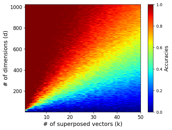
(a) HRR(w/Proj)

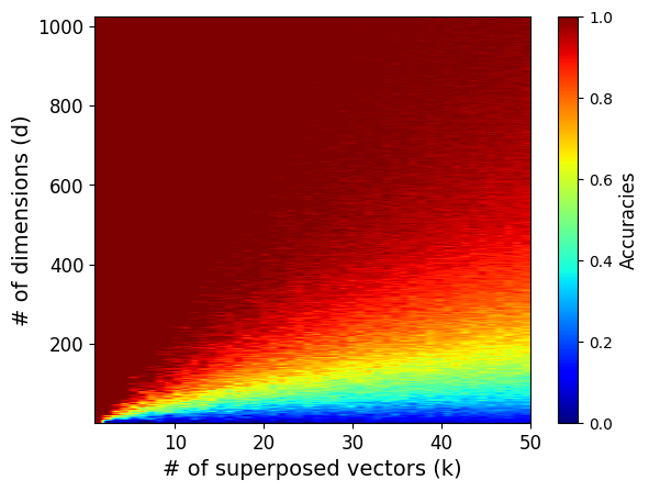
(b) CHRR

Figure 2: Retrieval accuracies of HRR(w/Proj) and CHRR. The number of dimensions $d$ was $1,\dots,1024$ and the number of positive classes $k$ was $1,\dots,50$.

We experimentally demonstrated CHRR’s capacity by comparing its retrieval accuracy with that of HRR. The experiment attempted to verify how accurately the positive class vector can be retrieved from a memory vector. For a data instance $x$, let $\mathbf{c}_{p}$ be a vector for a positive class $p$ to which $x$ belongs, and let $\mathbf{p}$ be a vector for the positive class concept label. The binding and superposition operations allow us to represent all positive classes for $x$ as $\mathbf{R}$:

$$\mathbf{R}=\bigoplus_{p\in\mathcal{Y}_{x}}(\mathbf{p}\otimes\mathbf{c}_{p}).$$ (6)

In the experiment, we generated a database consisting of $N=1,000$ random $d$-dimensional vectors ($\mathbf{c}_{j}\in\mathbb{R}^{d}$, for all $j\in[1,\dots,N]$). Then, to create $\mathbf{R}$, we randomly selected $k$ vectors from the database to be $\mathbf{c}_{p}$ and one vector to be $\mathbf{p}$. As shown in Equation 6, the $k$ associations can be superposed to represent $\mathbf{R}$. To retrieve $\mathbf{c}_{p}$ from $\mathbf{R}$, we used the unbinding operation to decode a noisy version of the vector $\mathbf{c}_{p}$ from $\mathbf{R}$, as $\hat{\mathbf{c}}_{p}=\mathbf{R}\otimes\mathbf{p}^{\dagger}$. For each $j\in[1,\dots,N]$, we computed the similarity $s_{j}=sim(\hat{\mathbf{c}}_{p},\mathbf{c}_{j})$ between the decoded vector $\hat{\mathbf{c}}_{p}$ and the individual vector $\mathbf{c}_{j}$. After that, we compiled the top-$k$ label list according to the similarity scores $s_{j}$. To evaluate the retrieval accuracy, we measured the percentage of class labels in the list, whose vectors were encoded into the memory $\mathbf{R}$. By varying the number of dimensions $d=1,\dots,1024$ and the number of binding pairs $k=1,\dots,50$, we plotted the accuracies as a heat-map (Figure 2, where warmer colors indicate higher accuracy). The results clearly show that CHRR has better retrieval accuracies than those of HRR. Moreover, the larger the number of superposed vectors ($k$) is, the bigger the performance difference between CHRR and HRR becomes. Hence, this tendency indicates that CHRR is more suitable than HRR for encoding many labels.

3.3 Variance Comparison Experiment

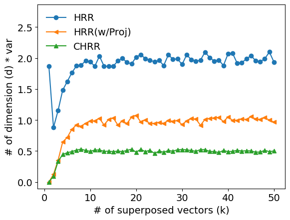
(a) Variance

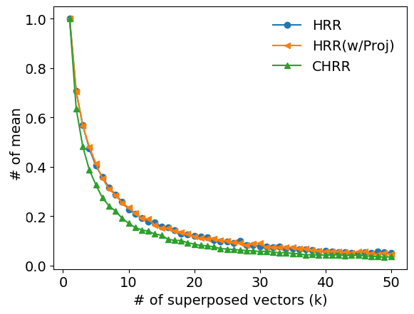
(b) Mean

Figure 3: Variance and mean of the similarities of HRR, HRR(w/Proj), and CHRR. We fixed the number of dimensions $d$ to $400$ and varied the number of positive classes $k$ from $1$ to $50$.

In  § 3.2, we confirmed that CHRR exhibits superior retrieval ability to HRR. There is a possibility that the CHRR’s similarity operation reduces the variance more than the projection does. The experiment reported below was conducted to check the numerical stability of the CHRR’s similarity operation. To create $\mathbf{R}$ as Equation 6, we generated $k$ random vectors $\mathbf{c}_{p}$ and $\mathbf{p}$. We extracted a noisy version of $\mathbf{c}_{p}$ from ${\mathbf{R}}$ as $\hat{\mathbf{c}}_{p}=\mathbf{R}\otimes\mathbf{p}^{\dagger}$. For each $j\in[1,\dots,k]$, we measure the similarity between $\mathbf{\hat{c}_{p}}$ and $\mathbf{c}_{j}$ as $s_{j}=sim(\mathbf{\hat{c}}_{p},\mathbf{c}_{j})$. We plotted the variances and means of the similarities in Figure 3 (a) and (b), respectively. We fixed the number of dimensions $d$ to $400$ and varied the number of binding pairs $k=1,\dots,50$. Our experiments compared three methods, CHRR, HRR proposed in (Plate, 1995), and HRR with the projection of (Ganesan et al., 2021) (HRR(w/Proj)).

Figure 3 (a) shows that as $k$ increases, the variances of all methods tend to converge. However, while the variance converges, the mean also decreases near zero, as shown in Figure 3 (b). Therefore, as the number of superposed vectors $k$ increases, the impact of variance becomes relatively larger. Regarding the variance, we can see the need for the projection, since the HRR(w/Proj) is more suppressed than the original HRR. Yet, we found that CHRR is most suppressed; that is, CHRR is more numerically stable than HRR(w/Proj). As for the mean, the three methods had roughly comparable performances. Although the mean approached zero as $k$ increased, this is not a problem in using similarity for compiling a ranking list of labels.

4 Neural Network Architecture

One of the challenges in adapting CHRR to XMC tasks is how to adapt the output layer of DNN models to a circular vector because it has a cyclic feature; i.e., $\theta=2\pi n\times\theta$, where $n\in\mathbb{Z}$. To meet it, we developed a neural network for predicting angles that considers the cyclic feature during the training. The key idea was to represent the output in Cartesian coordinates, which can uniquely represent a point on a unit circle. Then, we converted the output into polar coordinates to obtain angles.

4.1 Architecture for Circular Vectors

We used fully connected (FC) networks in all of the experiments. They were each composed of a $F$-dimensional input layer, two $h$-dimensional hidden layers with ReLU activation (Agarap, 2018), and a $d^{\prime}$-dimensional output layer. That is, they had the same architecture except for the output layer.

We selected two baselines from Ganesan et al. (2021) by using the FC networks. The first baseline had $L$ output nodes and each node is used to binary classification (we refer to it below as FC). The second baseline was the method using HRR as described in § 2.2. It had $d$ output nodes (we refer to it below as HRR).

Our network for CHRR represented a pair of the outputs as a point on a unit circle on Cartesian coordinates; i.e., $(\cos\phi,\sin\phi)$, as shown in Figure 1. Then we converted the point into polar coordinates $(1,\phi)$, and used $\phi$ as an element of the predicted label vector. Let $\hat{\mathbf{s}}\in\mathbb{R}^{2d}$ be the raw output vector, and $\hat{\mathbf{S}}\in\mathbb{C}^{d}$ be the converted circular vector. We represented $d$ pairs from $\hat{\mathbf{s}}$ in Cartesian coordinates as $a_{i}=(x_{i},y_{i})$. Then, we normalized them to satisfy $\|a_{i}\|=1$. Although there was a similar work for an angle prediction using a neural network (Heffernan et al., 2015), they used $\arctan{\frac{y}{x}}$ for the conversion whose range was limited to $\left[\frac{-\pi}{2},\frac{\pi}{2}\right]$. Instead, we used the atan2 function (Organick, 1966), which can convert a $(x,y)$ point to a corresponding angle $(-\pi,\pi]$. Finally, we adapted the atan2 to $a_{i}$ to obtain $\hat{S}_{i}$. We named this method as CHRR.

4.2 Impact of Model Architecture

Because the number of the output nodes of CHRR ($2d$) is twice as that of HRR ($d$), the total model size of CHRR also increases. Therefore, we conducted two different experiments using the same model size as HRR (see § 5.4 for the results). The first experiment changed the network architecture of CHRR. Figure 4 compares the architectures of CHRR and the changed model (CHRR-Half) to illustrate the impact of halving the hidden and output layer sizes on model performance. This adjustment ensures that CHRR-Half has the same number of parameters as HRR, allowing for a fair comparison. We made CHRR-Half by splitting the second hidden layer’s nodes and output nodes of CHRR in half. This resulted in two sets of $\frac{h}{2}$ hidden nodes and $d$ output nodes. Then we connected one set of hidden nodes to one set of output nodes, and the other set of hidden nodes to the other set of output nodes. As a result, $2\times(\frac{h}{2}\times d)=h\times d$ parameters were obtained, which equals the number of parameters between the second hidden layer and the output layer in HRR. The results of the experiment in § 5.4 showed no significant difference in performance between CHRR and this model. Therefore, the increase in the model size is not a big issue. In the second experiment, to demonstrate the advantage of the proposed architecture against naive implementation, we used the same network architecture as HRR, and mapped the real-valued outputs to angles with activation functions. We tried two activation functions, $\sin$ and $\tanh$ to map the outputs to $[-1,1]$; then the output was multiplied by $\pi$ to obtain $(-\pi,\pi]$ outputs. We named these models as CHRR-sin and CHRR-tanh. Both showed more modest levels of performance compared with CHRR.

(a) CHRR

(b) CHRR-Half

Figure 4: Comparison of CHRR and CHRR-Half architectures.

5 Experiment on XMC Datasets

To examine the advantages of circular vectors, we conducted experiments on several XMC datasets. Note that achieving the state-of-the-art performance on XMC datasets was not the goal of this study, which focuses on the efficiency of the learning method with circular vectors. However, to validate the effectiveness of CHRR in the XMC task, we compared our method with several strong baselines. These include tree-based FastXML Prabhu and Varma (2014), PfastreXML Prabhu et al. (2018a), and deep learning based XML-CNN Zhang et al. (2018), in addition to FC and HRR.

5.1 Datasets

Dataset	$N_{train}$	$N_{test}$	$L$	$\bar{L}$
Delicious	12,920	3,185	983	311.61
EURLex-4K	15,539	3,809	3,993	25.73
Wiki10-31K	14,146	6,616	101,938	8.52
Delicious-200K	196,606	100,095	205,443	2.29

Table 2: Details of the datasets from Bhatia et al. (2016). Here, $N_{train}$ is the number of training samples, $N_{test}$ is the number of test samples, $L$ is the number of labels, $\bar{L}$ is the average number of samples per label.

We evaluated our method on the four datasets for text XMC tasks from Bhatia et al. (2016). Table 2 shows the details of the datasets. The features for each sample is a bag-of-words of $F$ words.

5.2 Evaluation Metrics

We evaluated each method by using precision at $k$ (P@$k=\frac{1}{k}\sum_{l\in\text{rank}_{k}(\hat{\mathbf{y}})}\mathbf{y}_{l}$) and the propensity score at $k$ (PSP@$k$), which are commonly used metrics in the XMC task. P@$k$ is the proportion of true labels in the top-$k$ predictions. PSP@$k=\frac{1}{k}\sum_{l\in\text{rank}_{k}(\hat{\mathbf{y}})}\frac{\mathbf{y}_{l}}{p_{l}}$ is a variation of precision that takes into account the relative frequency of each label. Here, $\text{rank}_{k}(\hat{\mathbf{y}})$ is the ranking of all labels in the predicted $\hat{\mathbf{y}}$ and $p_{l}$ is the relative frequency of the $l$-th label. We used $k=1,5,10,20$ for P@$k$, and $k=1,5,10,20$ for PSP@$k$ in the experiments described below.

5.3 Experimental Settings

	Delicious ($\textbf{59\%},\textbf{19\%}$)				Delicious-200K ($\textbf{61\%},\textbf{80\%}$)
	P@1	P@5	PSP@1	PSP@5	P@1	P@5	PSP@1	PSP@5
FastXML	69.6	59.3	32.3	35.4	43.1	36.2	6.5	8.3
PfastreXML	67.1	58.6	34.6	35.9	41.7	35.6	3.2	4.4
FC	70.8	59.2	34.1	36.1	35.1	32.1	5.3	7.4
CHRR	71.2	59.3	34.3	35.9	43.2	37.1	6.6	8.5
	EURLex-4K ($\textbf{61\%},\textbf{99\%}$)				Wiki10-31K ($\textbf{62\%},\textbf{99\%}$)
	P@1	P@5	PSP@1	PSP@5	P@1	P@5	PSP@1	PSP@5
FastXML	76.4	52.0	33.2	42.0	83.0	57.8	9.8	10.5
PfastreXML	71.4	50.4	26.6	39.0	83.6	59.1	19.0	18.4
XML-CNN	75.3	49.2	32.4	39.5	81.4	56.1	9.4	10.2
FC	77.4	47.9	33.6	37.3	80.5	46.4	10.5	8.9
FC$+\phi_{\text{XLNet}}$	73.3	48.8	33.0	40.0	84.0	58.9	10.9	11.5
CHRR	75.2	47.8	28.7	34.9	82.2	58.8	10.2	10.9
CHRR$+\phi_{\text{XLNet}}$	77.0	50.0	29.8	37.6	86.8	65.1	11.9	13.0

Table 3: Performance comparisons of CHRR and other competing methods over four benchmark datasets, and the left number in bold represents the compression ratio $\left(1-\frac{(F\times h_{C}+{h_{C}}\times{h_{C}})+(h_{C}\times 2d+d\times L)}{(F\times h_{F}+{h_{F}}\times{h_{F}})+(h_{F}\times L)}\right)$ of the CHRR’s model size for FC’s model size. CHRR is set with $d=800$ and $h_{C}=768$. And the right number in bold represents the compression ratio ($1-\frac{d}{L}$) of the CHRR’s output dimensions for FC’s output dimensions. For FC, $d$ is set at the number of labels in each dataset ($L$) and $h$ is set at $2048$. FC$+\phi_{\text{XLNet}}$ and CHRR$+\phi_{\text{XLNet}}$ refers to the results obtained using XLNet as the feature representation. We obtained the results for FastXML, PfastreXML, and XML-CNN from You et al. (2019) and Yu et al. (2022).

We compared CHRR to five competitive methods (FC, HRR, FastXML, PfastreXML, XML-CNN) over four datasets. For the implementation of FC and HRR, we used the scripts provided by Ganesan et al. (2021) available at the GitHub URL. We implemented CHRR by using PyTorch (Paszke et al., 2019). The training methods and the model architectures basically followed the scripts provided by Ganesan et al. (2021). The learning rate was set to 1, the batch size was 64, and the number of training epochs was 100. These hyperparameters were chosen based on preliminary experiments to balance training time and model performance. For the EURLex-4K and Wiki10-31K datasets, we also conducted experiments using both BoW (Bag of Words) and pretrained XLNet embeddings Chang et al. (2020) as features. The dimensionality of BoW is the same as the dimensionality $F$ of the features shown in Table 2, and the dimensionality of XLNet as a feature is $1,024$ dimensions. In CHRR, we varied the dimension of the symbol vectors ($d$) $\{100,400,800,1000\}$. To investigate the possibility that a larger hidden layer size $h$ improves the learning effect in FCs with large output dimensionality, we conducted experiments with three settings of hidden layer size ($h$) $\{768,1024,2048\}$. For main results, we chose $d=800$ and $h=768$ for CHRR and $h=2048$ for FC. All experiments are conducted with two hidden layers.

5.4 Results and Discussion

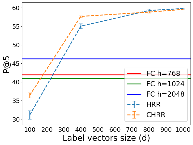
(a) Wiki10-31K P@5

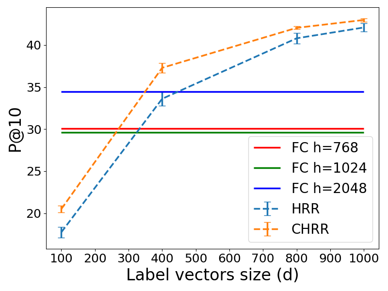
(b) Wiki10-31K P@10

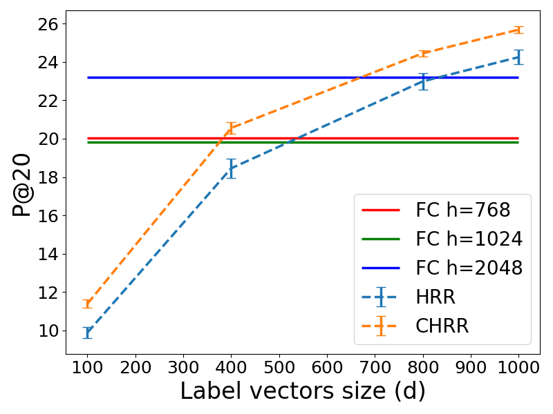
(c) Wiki10-31K P@20

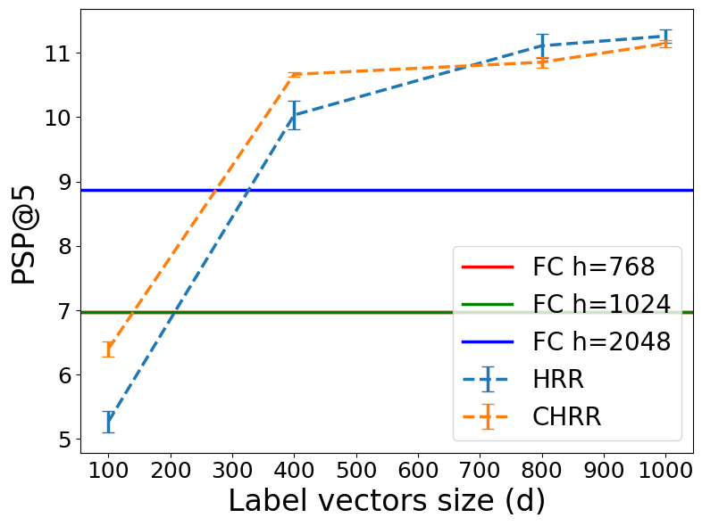
(d) Wiki10-31K PSP@5

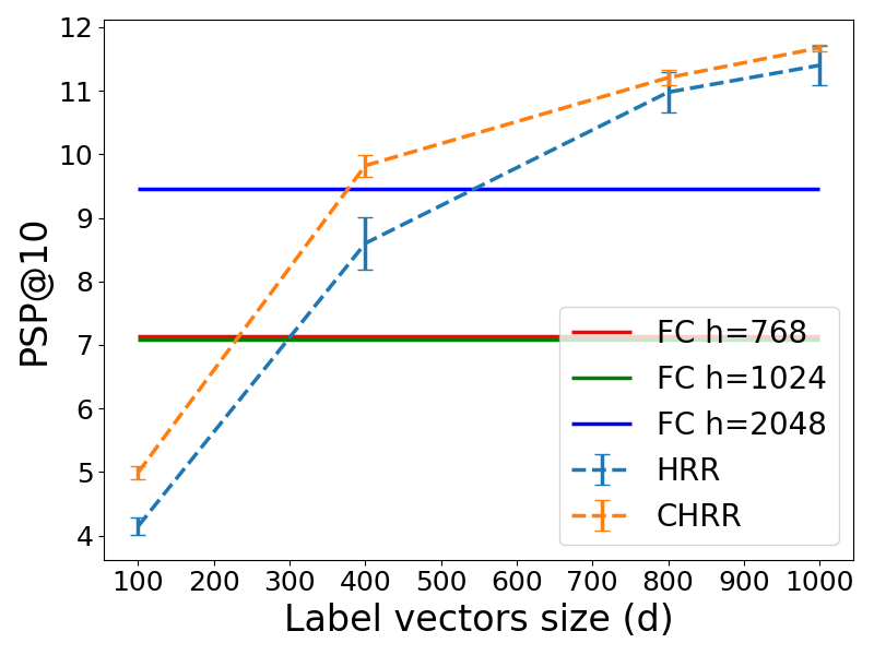
(e) Wiki10-31K PSP@10

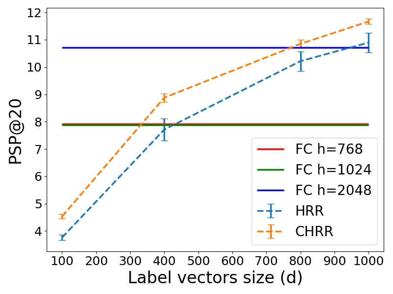
(f) Wiki10-31K PSP@20

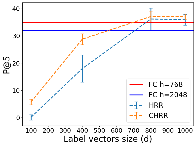
(g) Delicious-200K P@5

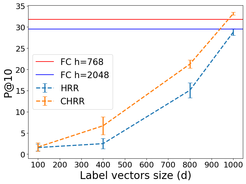
(h) Delicious-200K P@10

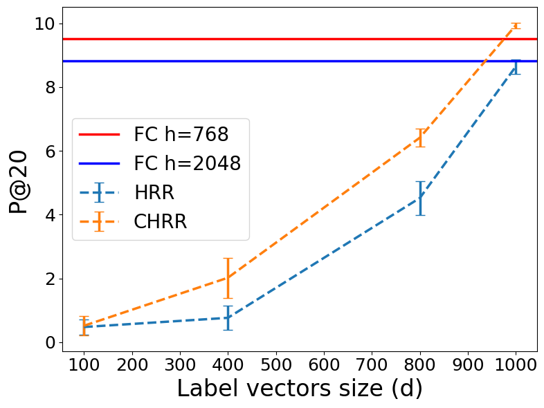
(i) Delicious-200K P@20

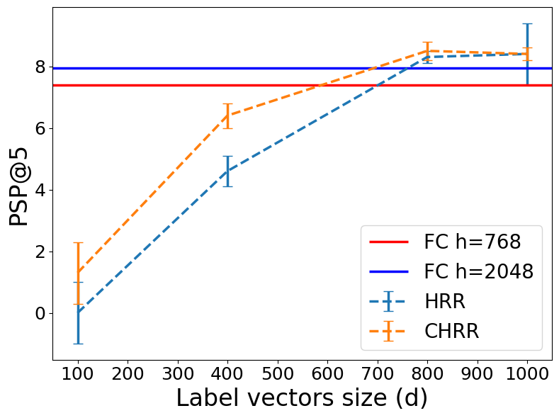
(j) Delicious-200K PSP@5

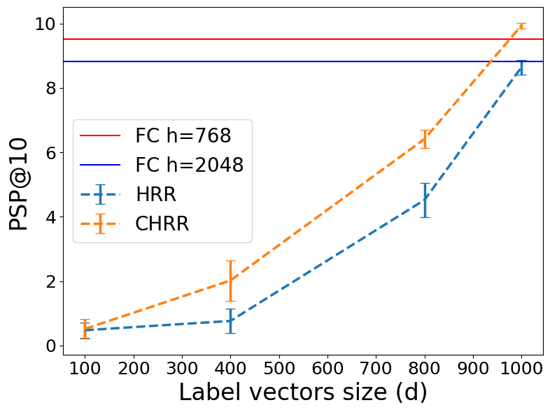
(k) Delicious-200K PSP@10

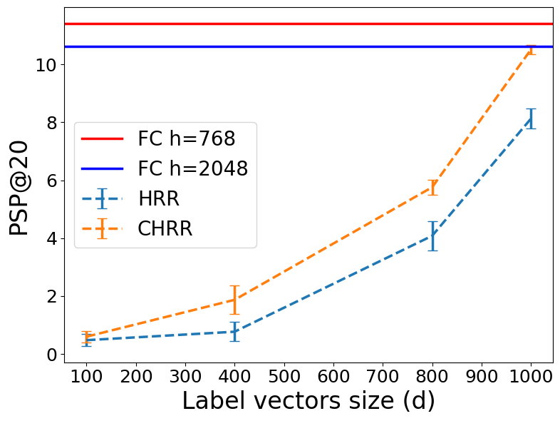
(l) Delicious-200K PSP@20

Figure 5: Impact of the number of dimensions ($d$) on P@5, P@10, P@20, PSP@5, PSP@10, and PSP@20 for Wiki10-31K and Delicious-200K datasets. We used BoW as features in all models.

Table 3 lists P@1, P@5, PSP@1, and PSP@5 for the CHRR model, with five standard methods. CHRR achieves up to 99% output dimension compression and 62% model size reduction compared to FC, which is comparable or better than other baselines. CHRR$+\phi_{\text{XLNet}}$ with XLNet as a feature showed higher results than the CHRR case with BoW. In particular, it showed significant improvement on the Wiki10-31K dataset. Figure 5 shows the impact of the dimensionality size $d$ of the HRR and CHRR on performance, in addition to the FC results. On certain datasets, CHRR outperformed FC even when it had vectors with lower dimensions. These results suggest that CHRR has a higher capacity for learning on datasets with a large number of labels than FC does.

We also compared CHRR with HRR. As shown in Figure 5, CHRR was better than HRR in many cases. In particular, the results for P@20 and PSP@20, where the value of the evaluation index k is large, we confirmed that the difference in performance is significant. As our theoretical experiment in § 3.2 showed, CHRR could represent many labels with high accuracy even for low-dimensional vectors. The results of the theoretical experiments in § 3.2 and the experiment on real datasets in § 5 suggest that the CHRR is able to represent a larger number of correct labels.

5.5 Impact of Model Architecture

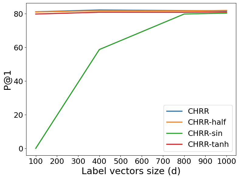
(a) P@1

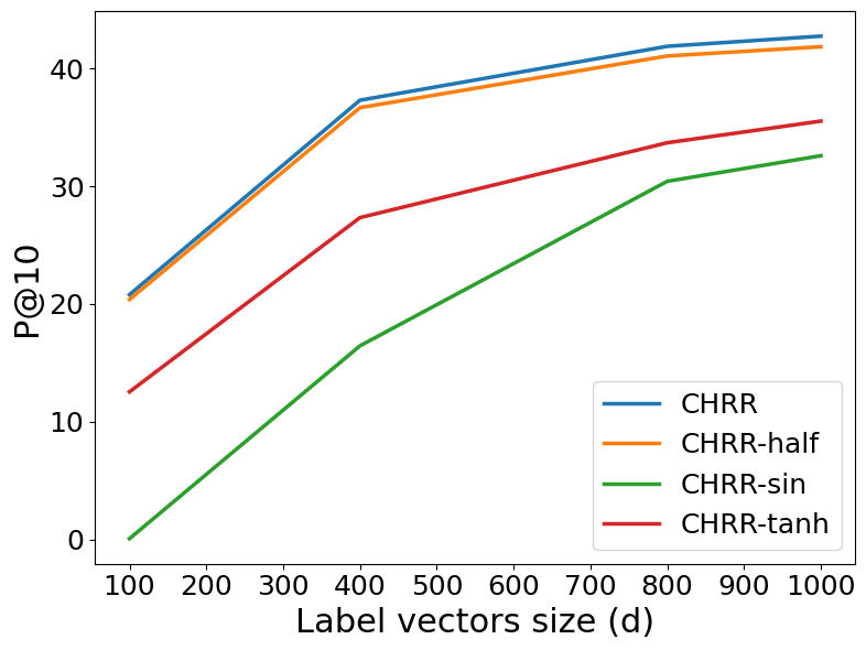
(b) P@10

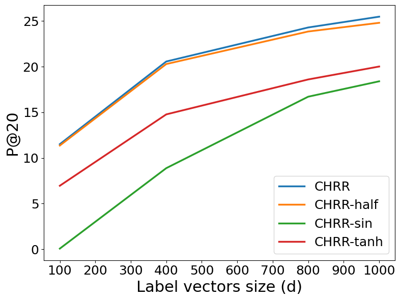
(c) P@20

Figure 6: Comparison of CHRR variants (CHRR, -Half, -sin, and -tanh) on the Wiki10-31K dataset.

This section describes the results of the experiments on the impact of the model architectures in § 4.2. Figure 6 compares the performances of the CHRR variants (CHRR, CHRR-Half, CHRR-sin, and CHRR-tanh) on the Wiki10-31K dataset. As mentioned in § 4.2, there was no significant difference in performance between CHRR and this model. CHRR-sin and CHRR-tanh both obtained similar results that were inferior to those of CHRR and CHRR-Half. While the $\sin$ function in CHRR-sin seems to consider the cyclic feature, the results show that it is imperfect at predicting the of the circular-label vector. In short, our developed network architecture is important for the XMC learning with circular vectors, while the increase in the model size is not a big issue.

6 Conclusion

The XMC task still faces challenge of dealing with a large number of output labels. In this paper, we attempted to address this issue by using a low dimensional circular vector to output directly. In theoretical experiments in § 3.2 and § 3.3, we showed that many labels can be accurately encoded by using circular vectors (CHRR) rather than normal real-valued vectors (HRR). Moreover, using actual XMC datasets, we compared CHRR with baseline methods in § 5. CHRR reduced the output layer size by up to 99% compared to FC, while it outperformed other baselines in most results. Comparing HRR and CHRR, CHRR outperformed on most results. In the future, we will incorporate circular vector systems into other DNN models such as LSTM (Hochreiter and Schmidhuber, 1997) and Transformer (Vaswani et al., 2017), as well as Associative LSTM (Danihelka et al., 2016) and Hrrformer (Alam et al., 2023).

Limitations

Our study has several limitations that should be considered in interpreting the results:

1. Model Age and Adaptability: The HRR and CHRR models utilized in our experiments are based on established frameworks that may not incorporate the latest advancements in neural network architectures Ganesan et al. (2021). Newer models or hybrid approaches might offer improved performance.

2. Comparison with State-of-the-Art XMC Models: Our study did not include a comparison with the latest models in the Extreme Multi-label Classification (XMC) domain, such as APLC-XLNet Ye et al. (2020), LightXML Jiang et al. (2021), AttentionXML You et al. (2019), and CascadeXML Kharbanda et al. (2022). Future research should consider comparing the performance of HRR, HRR(w/Proj), and CHRR against these state-of-the-art models to provide a more comprehensive evaluation of their effectiveness in .

3. Comparison with LLM: Our study did not include a comparison with the Large Language Model (LLM) approach, which is currently the state-of-the-art in various NLP tasks. Future research should consider comparing the performance of HRR, HRR(w/Proj), and CHRR against LLMs to further evaluate the effectiveness of these models.

These limitations underscore the need for further research to refine and extend the applicability of the models proposed in this study.

Ethics Statement

We used the publicly available XMC datasets, Delicious, EURLex-4K, Wiki10-31K and Delicious-200K, to train and evaluate DNN models, and there is no ethical consideration.

Reproducibility Statement

As mentioned in § 5.3, we used the publicly available code to implement FC, HRR and CHRR. Our code will be available at https://github.com/Nishiken1/Circular-HRR.

References

- Agarap (2018) Abien Fred Agarap. 2018. Deep learning using rectified linear units (relu). arXiv preprint arXiv:1803.08375.
- Alam et al. (2023) Mohammad Mahmudul Alam, Edward Raff, Stella Biderman, Tim Oates, and James Holt. 2023. Recasting self-attention with holographic reduced representations. arXiv preprint arXiv:2305.19534.
- Babbar and Schölkopf (2017) Rohit Babbar and Bernhard Schölkopf. 2017. Dismec: Distributed sparse machines for extreme multi-label classification. In Proceedings of the tenth ACM international conference on web search and data mining, pages 721–729.
- Bhatia et al. (2016) K. Bhatia, K. Dahiya, H. Jain, P. Kar, A. Mittal, Y. Prabhu, and M. Varma. 2016. The extreme classification repository: Multi-label datasets and code.
- Chang et al. (2020) Wei-Cheng Chang, Hsiang-Fu Yu, Kai Zhong, Yiming Yang, and Inderjit S Dhillon. 2020. Taming pretrained transformers for extreme multi-label text classification. In Proceedings of the 26th ACM SIGKDD international conference on knowledge discovery & data mining, pages 3163–3171.
- Dahiya et al. (2023) Kunal Dahiya, Nilesh Gupta, Deepak Saini, Akshay Soni, Yajun Wang, Kushal Dave, Jian Jiao, Gururaj K, Prasenjit Dey, Amit Singh, et al. 2023. Ngame: Negative mining-aware mini-batching for extreme classification. In Proceedings of the Sixteenth ACM International Conference on Web Search and Data Mining, pages 258–266.
- Danihelka et al. (2016) Ivo Danihelka, Greg Wayne, Benigno Uria, Nal Kalchbrenner, and Alex Graves. 2016. Associative long short-term memory. CoRR, abs/1602.03032.
- Dekel and Shamir (2010) Ofer Dekel and Ohad Shamir. 2010. Multiclass-multilabel classification with more classes than examples. In Proceedings of the Thirteenth International Conference on Artificial Intelligence and Statistics, pages 137–144. JMLR Workshop and Conference Proceedings.
- Deng et al. (2010) Jia Deng, Alexander C Berg, Kai Li, and Li Fei-Fei. 2010. What does classifying more than 10,000 image categories tell us? In Computer Vision–ECCV 2010: 11th European Conference on Computer Vision, Heraklion, Crete, Greece, September 5-11, 2010, Proceedings, Part V 11, pages 71–84. Springer.
- Ganesan et al. (2021) Ashwinkumar Ganesan, Hang Gao, Sunil Gandhi, Edward Raff, Tim Oates, James Holt, and Mark McLean. 2021. Learning with holographic reduced representations. Advances in Neural Information Processing Systems, 34:25606–25620.
- Gayler (2004) Ross W Gayler. 2004. Vector symbolic architectures answer jackendoff’s challenges for cognitive neuroscience. arXiv preprint cs/0412059.
- Hayashi and Shimbo (2017) Katsuhiko Hayashi and Masashi Shimbo. 2017. On the equivalence of holographic and complex embeddings for link prediction. In Proceedings of the 55th Annual Meeting of the Association for Computational Linguistics (Volume 2: Short Papers), pages 554–559, Vancouver, Canada. Association for Computational Linguistics.
- Heffernan et al. (2015) Rhys Heffernan, Kuldip Paliwal, James Lyons, Abdollah Dehzangi, Alok Sharma, Jihua Wang, Abdul Sattar, Yuedong Yang, and Yaoqi Zhou. 2015. Improving prediction of secondary structure, local backbone angles and solvent accessible surface area of proteins by iterative deep learning. Scientific Reports, 5(1):11476.
- Hochreiter and Schmidhuber (1997) Sepp Hochreiter and Jürgen Schmidhuber. 1997. Long short-term memory. Neural computation, 9(8):1735–1780.
- Jain et al. (2016) Himanshu Jain, Yashoteja Prabhu, and Manik Varma. 2016. Extreme multi-label loss functions for recommendation, tagging, ranking & other missing label applications. In Proceedings of the 22nd ACM SIGKDD international conference on knowledge discovery and data mining, pages 935–944.
- Jain et al. (2023) Vidit Jain, Jatin Prakash, Deepak Saini, Jian Jiao, Ramachandran Ramjee, and Manik Varma. 2023. Renee: End-to-end training of extreme classification models. Proceedings of Machine Learning and Systems, 5.
- Jiang et al. (2021) Ting Jiang, Deqing Wang, Leilei Sun, Huayi Yang, Zhengyang Zhao, and Fuzhen Zhuang. 2021. Lightxml: Transformer with dynamic negative sampling for high-performance extreme multi-label text classification. In Proceedings of the AAAI Conference on Artificial Intelligence, volume 35, pages 7987–7994.
- Kanerva (1996) Pentti Kanerva. 1996. Binary spatter-coding of ordered k-tuples. In International Conference on Artificial Neural Networks.
- Khandagale et al. (2020) Sujay Khandagale, Han Xiao, and Rohit Babbar. 2020. Bonsai: diverse and shallow trees for extreme multi-label classification. Machine Learning, 109:2099–2119.
- Kharbanda et al. (2022) Siddhant Kharbanda, Atmadeep Banerjee, Erik Schultheis, and Rohit Babbar. 2022. Cascadexml: Rethinking transformers for end-to-end multi-resolution training in extreme multi-label classification.
- Liu et al. (2017) Jingzhou Liu, Wei-Cheng Chang, Yuexin Wu, and Yiming Yang. 2017. Deep learning for extreme multi-label text classification. In Proceedings of the 40th international ACM SIGIR conference on research and development in information retrieval, pages 115–124.
- Mikolov et al. (2013) Tomas Mikolov, Kai Chen, Greg Corrado, and Jeffrey Dean. 2013. Efficient estimation of word representations in vector space. arXiv preprint arXiv:1301.3781.
- Nickel et al. (2016) Maximilian Nickel, Lorenzo Rosasco, and Tomaso Poggio. 2016. Holographic embeddings of knowledge graphs. In Proceedings of the AAAI conference on artificial intelligence, volume 30.
- Organick (1966) EI Organick. 1966. Some processors also offer the library function called atan2 a function of two arguments (opposite and adjacent). In A FORTRAN IV Primer, page 42. Addison-Wesley.
- Partalas et al. (2015) Ioannis Partalas, Aris Kosmopoulos, Nicolas Baskiotis, Thierry Artieres, George Paliouras, Eric Gaussier, Ion Androutsopoulos, Massih-Reza Amini, and Patrick Galinari. 2015. Lshtc: A benchmark for large-scale text classification. arXiv preprint arXiv:1503.08581.
- Paszke et al. (2019) Adam Paszke, Sam Gross, Francisco Massa, Adam Lerer, James Bradbury, Gregory Chanan, Trevor Killeen, Zeming Lin, Natalia Gimelshein, Luca Antiga, et al. 2019. Pytorch: An imperative style, high-performance deep learning library. Advances in neural information processing systems, 32.
- Plate (1992) Tony A Plate. 1992. Holographic recurrent networks. Advances in neural information processing systems, 5.
- Plate (1995) Tony A Plate. 1995. Holographic reduced representations. IEEE Transactions on Neural networks, 6(3):623–641.
- Plate (2003) Tony A Plate. 2003. Holographic Reduced Representation: Distributed representation for cognitive structures, volume 150. CSLI Publications Stanford.
- Prabhu et al. (2018a) Y. Prabhu, A. Kag, S. Gopinath, K. Dahiya, S. Harsola, R. Agrawal, and M. Varma. 2018a. Extreme multi-label learning with label features for warm-start tagging, ranking and recommendation. In Proceedings of the ACM International Conference on Web Search and Data Mining.
- Prabhu and Varma (2014) Y. Prabhu and M. Varma. 2014. Fastxml: A fast, accurate and stable tree-classifier for extreme multi-label learning. In Proceedings of the ACM SIGKDD Conference on Knowledge Discovery and Data Mining.
- Prabhu et al. (2018b) Yashoteja Prabhu, Anil Kag, Shrutendra Harsola, Rahul Agrawal, and Manik Varma. 2018b. Parabel: Partitioned label trees for extreme classification with application to dynamic search advertising. In Proceedings of the 2018 World Wide Web Conference, pages 993–1002.
- Rachkovskij (2001) D.A. Rachkovskij. 2001. Representation and processing of structures with binary sparse distributed codes. IEEE Transactions on Knowledge and Data Engineering, 13(2):261–276.
- Ridnik et al. (2021) Tal Ridnik, Emanuel Ben-Baruch, Asaf Noy, and Lihi Zelnik-Manor. 2021. Imagenet-21k pretraining for the masses. arXiv preprint arXiv:2104.10972.
- Schlegel et al. (2021) Kenny Schlegel, Peer Neubert, and Peter Protzel. 2021. A comparison of vector symbolic architectures. Artificial Intelligence Review, 55(6):4523–4555.
- Smolensky (1990) Paul Smolensky. 1990. Tensor product variable binding and the representation of symbolic structures in connectionist systems. Artificial intelligence, 46(1-2):159–216.
- Vaswani et al. (2017) Ashish Vaswani, Noam Shazeer, Niki Parmar, Jakob Uszkoreit, Llion Jones, Aidan N Gomez, Łukasz Kaiser, and Illia Polosukhin. 2017. Attention is all you need. Advances in neural information processing systems, 30.
- Wydmuch et al. (2018) Marek Wydmuch, Kalina Jasinska, Mikhail Kuznetsov, Róbert Busa-Fekete, and Krzysztof Dembczynski. 2018. A no-regret generalization of hierarchical softmax to extreme multi-label classification. Advances in neural information processing systems, 31.
- Ye et al. (2020) Hui Ye, Zhiyu Chen, Da-Han Wang, and Brian D. Davison. 2020. Pretrained generalized autoregressive model with adaptive probabilistic label clusters for extreme multi-label text classification.
- You et al. (2019) Ronghui You, Zihan Zhang, Ziye Wang, Suyang Dai, Hiroshi Mamitsuka, and Shanfeng Zhu. 2019. Attentionxml: Label tree-based attention-aware deep model for high-performance extreme multi-label text classification. Advances in Neural Information Processing Systems, 32.
- Yu et al. (2022) Hsiang-Fu Yu, Kai Zhong, Jiong Zhang, Wei-Cheng Chang, and Inderjit S. Dhillon. 2022. Pecos: Prediction for enormous and correlated output spaces.
- Zanzotto and Dell’Arciprete (2012) Fabio Massimo Zanzotto and Lorenzo Dell’Arciprete. 2012. Distributed tree kernels. In Proceedings of the 29th International Coference on International Conference on Machine Learning, pages 115–122.
- Zhang et al. (2021) Jiong Zhang, Wei-Cheng Chang, Hsiang-Fu Yu, and Inderjit Dhillon. 2021. Fast multi-resolution transformer fine-tuning for extreme multi-label text classification. Advances in Neural Information Processing Systems, 34:7267–7280.
- Zhang et al. (2018) Wenjie Zhang, Junchi Yan, Xiangfeng Wang, and Hongyuan Zha. 2018. Deep extreme multi-label learning.